Abstract
Accurate and reliable estimation information of sideslip angle is very important for intelligent motion control and active safety control of an autonomous vehicle. To solve the problem of sideslip angle estimation of an autonomous vehicle, a sideslip angle fusion estimation method based on robust cubature Kalman filter and wheel-speed coupling relationship is proposed in this paper. The vehicle dynamics model, tire model, and wheel speed coupling model are established and discretized, and a robust cubature Kalman filter is designed for vehicle running state estimation according to the discrete vehicle model. An adaptive measurement-update solution of the robust cubature Kalman filter is presented to improve the robustness of estimation, and then, the wheel-speed coupling relationship is introduced to the measurement update equation of the robust cubature Kalman filter and an adaptive sideslip angle fusion estimation method is designed. The simulations in the CarSim-Simulink co-simulation platform and the actual vehicle road test are carried out, and the effectiveness of the proposed estimation method is validated by corresponding comparative analysis results.
1. Introduction
With the development of the automobile industry, people have higher and higher requirements for active safety and ride comfort of automobiles [1,2,3], and many advanced electronic control systems, such as electronic stabilization system, anti-lock braking system, traction control system, and anti-skid drive system, have been widely used in vehicles [4,5]. In these electronic control systems, accurate and reliable vehicle driving state measurement signal is one of the necessary conditions for closed-loop feedback control [6,7,8]. Over the past decade, the research on intelligent transportation and autonomous vehicles has been paid close attention to by the whole industry and has made vigorous developments [9,10,11,12]. In the process of intelligent driving of a vehicle, the driving state of a vehicle, especially the vehicle sideslip angle, is very important for vehicle motion control and is closely related to vehicle stability control effect. However, the vehicle sideslip angle is not easily measured directly, and expensive sensors are usually needed [13,14,15]. In this case, researchers in the automotive field tend to design corresponding vehicle sideslip angle estimators based on the vehicle model to calculate the size of the sideslip angle dynamically, thus as to replace the corresponding vehicle-mounted sensors [16,17,18,19]. Martin et al. [20] proposed a modular vehicle side-slip angle estimation method using a Kalman filter and applied it on a banked and low-friction road.
In recent years, remarkable progress has been made in the research of vehicle driving state estimation [21,22,23], including the estimation method of vehicle sideslip angle. In the actual driving process, vehicle parameters such as tire cornering stiffness are time-varying. These time-varying factors will cause very obvious non-linear interference in the vehicle model [24,25], which may directly lead to a large deviation or even failure of the designed estimator. Consequently, it is necessary to design a robust observer with the parameter perturbation being considered in vehicle state estimation. Zhang et al. [26] established a nonlinear vehicle dynamic model with the time-varying characteristics of vehicle parameters being considered, and designed a novel vehicle sideslip angle estimation method using the finite-frequency H∞ approach to improve the robustness of estimation results.
Vehicle in motion is a complex coupled driving system, and the coupling relationship and interaction between the different subsystems will affect the accuracy of estimation results [27,28,29]. With the deepening of research and the improvement of complexity, some researchers have begun to engage in the fusion estimation method of vehicle driving state, using different-model-based observers to iterate and compensate each other, using the preliminary estimation results to further approximate the real vehicle driving state, thereby improving the reliability and adaptive adjustment ability of the whole estimation system [30,31,32,33]. Li et al. [34,35] designed a series of fusion methods for vehicle sideslip angle estimation, which fused the observer based on vehicle kinematics model and the observer based on vehicle dynamics model and applied them to the iteration process of different Kalman filters, and designed corresponding adaptive adjustment methods to coordinate the weights of different observers. The simulation and experimental verification are carried out and the results show that the proposed fusion method has high estimation accuracy. Boada et al. [36] presented a vehicle sideslip angle estimation scheme on the basis of adaptive neuro-fuzzy inference system algorithm and unscented Kalman filter, using a sensor information fusion method to improve the estimation accuracy.
The Kalman filter and many of its improved algorithms are widely used in the research literatures of vehicle driving state estimation and many researchers have studied it extensively, which has been proved to be effective and dependable in practice [37,38,39,40]. Nam et al. [41] developed a novel sideslip angle and roll angle estimation method with lateral tire force being obtained by vehicular sensors directly, in which the recursive least squares and Kalman filter is applied to track the vehicle running states. Observing the existing research, we can find that the longitudinal acceleration, lateral acceleration, and yaw rate of the vehicle collected by a inertial navigation unit are usually used as the updated inputs of the measurement equation in vehicle driving state filtering estimation. However, once the state information measured by a single device or sensor fails or is disturbed by unknown external factors, it is easy to cause large deviations in the estimation results. Wheel speed coupling relationship is closely related to vehicle driving state, and wheel speed sensor price is relatively low, wheel speed information is relatively easy to obtain. If it is applied to vehicle state filtering estimation, the reliability of the whole estimation system can be improved by using redundancy of measurement information, which has great research value and space.
In this paper, a sideslip angle fusion estimation method of an autonomous vehicle is proposed based on robust cubature Kalman filter (RCKF) and wheel-speed coupling relationship. The three-degree-of-freedom vehicle model, tire model, and wheel-speed coupling model are established. The discretization form of a vehicle model is given, and a RCKF is designed based on the discrete vehicle model. Moreover, an adaptive measurement-update solution is presented to improve the robustness of estimation results. Then, a sideslip angle fusion estimation method is designed by reconstructing the measurement update equation using the wheel-speed coupling relationship, thus as to improve the accuracy and reliability of estimation results by using redundancy of measurement information.
The remainder of this paper is organized as follows. The vehicle model is presented in the Section 2. The vehicle sideslip angle fusion estimation method is designed in the Section 3. The simulation results are provided in the Section 4. The experimental verifications are shown in the Section 5, followed by the concluding remarks.
2. Vehicle Model
2.1. Three-Degree-of-Freedom Vehicle Dynamics Model
By fixing the origin of the dynamic coordinate system xoy on the autonomous vehicle and coinciding with the mass center of the vehicle, a three-degree-of-freedom vehicle model in the longitudinal, lateral, and yaw directions was established. The x axis and y axis represents the longitudinal and lateral axes respectively, and the x axis is positive in front and the y axis is positive in left. The angles and moments in the plane of all the coordinate systems are positive in the counterclockwise direction, and all vector components are positive in the same direction as the coordinate axis. It is considered that the mechanical properties of each tire are the same. The vertical motion of suspension and vehicle, the pitching motion of the automobile around the y axis, and the roll motion around the x axis are not considered in this paper. The three-degree-of-freedom vehicle dynamics model is shown in Figure 1, and the vehicle dynamics equation can be expressed as:
where vx is the longitudinal vehicle speed, vy is the lateral vehicle speed, γ is the yaw rate, m represents the vehicle mass, δ represents the steering angle of the front wheels, Iz stands for the moment of inertia. Fxj and Fyj (j = 1,2,3,4) are the longitudinal and lateral forces of the jth tire, respectively. lf and lr are the distances from the vehicle gravity center to the front and rear axle, respectively. bf and br are the half treads of the front wheels and rear wheels, respectively.
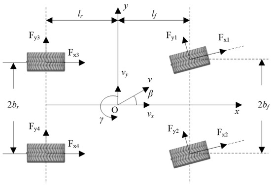
Figure 1.
Three-degree-of-freedom vehicle dynamics model.
2.2. Tire Model
In this paper, a semi-empirical magic formula tire model was used to characterize the tire force of the autonomous vehicle. The magic formula can be expressed as follows:
where Y(X) represents the longitudinal or lateral tire force, X is the tire slip rate s or tire sideslip angle α, B is the stiffness factor, C is the curve shape factor, D is the peak factor, E is the curve curvature factor, sh and sv are the horizontal and vertical offsets, respectively. The tire model parameters B, C, D, and E are all related to the vertical load of the tire. The vertical load of each tire is expressed as:
where Fz1, Fz2, Fz3, Fz4 represents vertical load of each corresponding tire, respectively. h is the height of vehicle mass center, g is the acceleration of gravity. The sideslip angle of each tire can be written as:
The tire slip rate can be obtained as:
where sj represents the tire slip rate of jth tire, nj represents the wheel rotating speed of jth tire, vnj represents the wheel linear velocity of jth tire, r represents the effective wheel radius. The coupling relationship of the four-wheel speed can be expressed as:
3. Vehicle Sideslip Angle Fusion Estimation Method
3.1. Robust Cubature Kalman Filter for Vehicle Running State Estimation
The vehicle dynamic model in Equations (1)–(3) can be expressed as the following discrete state space equation:
where xk represents the state space vector of discrete system, yk+1 represents the measurement vector of the discrete system, f(·) represents the state transfer function of discrete system, h(·) represents the measurement function of the discrete system, wk and vk represents the uncorrelated Gauss white noise. The system noise variance matrix Q and measurement noise variance matrix R can be computed as and , where is the Kronecker function. The discretization results of Equations (1)–(3) can be expressed as
where T represents the iterative step size of filter.
The cubature Kalman filter (CKF) is a nonlinear filter method with fixed sampling type, which has a higher estimation accuracy and real-time tracking ability. The traditional CKF algorithm is sensitive to the noise deviating from the true probability distribution. When the assumed Gauss noise deviates, the performance of the filter will be unstable or the estimation accuracy will be reduced. The Huber technique is an optimal estimation method with mixed norm as a cost function. It is robust to noise deviating from the assumed Gaussian distribution. The iteration steps of the robust CKF algorithm can be expressed as
(a) Initialization.
where is the initial state vector, is the error covariance matrix.
(b) Computation of sample points.
where i are the serial numbers of sample points, is obtained by Cholesky decomposing of and satisfy the condition of , represent the cubature points and can be computed by
(c) Time update.
Propagation of the cubature point.
Computation of the one-step predicted state.
(d) Measurement update.
Computation of Cholesky factorization.
Calculate the cubature points for the measurement update.
Propagation of the cubature point.
The predicted result of the measurement is computed as
The covariance matrix and cross-covariance matrix can be expressed as
The prediction error is given by
where is the actual value of k-time state, is the prediction value of k-time state. The measurement equation can be expressed as
where is the filter gain matrix and can be computed as .
3.2. Adaptive Measurement-Update Solution to Improve the Robustness of Estimation
The measurement update problem can be transformed into solving the following linear regression problem:
The state change matrix is selected as , then, the linear regression problem can be transformed as
where , , .
The measurement update problem of robust CKF equates to solving the minimum value of the following cost function:
where is the ith component of and , m is the dimension of , and can be denoted as
where is the adjusting parameter. The function is composed of 1-norm and 2-norm. When the adjusting parameter approaches to 0, the function approaches to the minimum of 1-norm. When the adjusting parameter approaches to infinity, the function approaches to the minimum of 2-norm. The application of function helps to enhance the robustness of estimation results. Solving the extreme value problem of cost function in Equation (27), we have
Denoting the function as and denoting the matrix as , and substituting the equation into Equation (29), we have
The iterative solution of Equation (30) is calculated as
where c is the iteration times. According to Equation (31), the measurement update of RCKF can be obtained. And then, the error covariance matrix in filter estimation is given by
3.3. Sideslip Angle Fusion Estimation Method Using Redundant Measurement Information
According to the nonlinear vehicle dynamics model in Equation (10), the vehicle running state can be estimated using the presented RCKF algorithm in the above chapter, in which the system state of RCKF is . In the existing literature regarding the filtering estimation method of the vehicle running state, the longitudinal and lateral vehicle acceleration is often selected as the actual measurement update input quantity of the designed filter, and the longitudinal and lateral vehicle acceleration can be expressed as
where ax and ay represents the longitudinal vehicle acceleration and lateral vehicle acceleration, respectively. In the tire model, the longitudinal vehicle acceleration and lateral vehicle acceleration are also closely related to the calculation results of tire forces. Once the sensor used to collect longitudinal and lateral vehicle acceleration has unpredictable deviation, it is easy to cause self-cycling and accumulation of estimation error, which makes the estimation results of filter gradually deviate from the actual values. To avoid this problem, the four-wheel rotational speed in Equation (8) is introduced and applied to the process of measurement-update iteration. According to Equation (8), one can find that the wheel-speed measurements will have a direct impact on the estimated results. Therefore, if the tire slips longitudinally, the estimation accuracy will be greatly reduced. According to this consideration, a reverse compensation method based on the tire slip rate is proposed to suppress the influence of tire slip on estimation results. The wheel-speed coupling relationship used as the measurement update equation can be rewritten as
where represents the original wheel-speed coupling relationship in Equation (8), represents the regulatory factor greater than 1, and is chosen as 1.2 in this paper. Then, the modified measurement equation with compensation effect can be expressed as
Using the RCKF algorithm in the above section, the vehicle running state observer can be designed. The measurement vector of RCKF is . It can be found that both the longitudinal and lateral acceleration can be used to estimate vehicle driving state, by adding the measurement information, the redundancy of measurement information is improved, and the redundancy of measurement information is conducive to improving the reliability and robustness of estimation results. Finally, the vehicle sideslip angle can be computed as
4. Simulation Results
In order to verify the performance of the proposed sideslip angle fusion estimation method of intelligent vehicle using RCKF and wheel-speed coupling relationship, a co-simulation model was built based on CarSim and Simulink software, and the simulation tests were carried out. The simulation results of EKF and RCKF were compared and analyzed. The simulation parameters in the simulation tests are shown in Table 1.

Table 1.
Vehicle parameters.
4.1. Case Study 1: Double Lane Changes Maneuver
The simulation conditions of the double lane change maneuver is shown in Figure 2, in which the vehicle speed was 25 m·s−1, the road adhesion coefficient was 1.0, the iterative step sizes of extend Kalman filter (EKF) and RCKF were 0.01 s, the initial state value was , the error covariance matrix was , the measurement noise covariance matrix was . The simulation results are shown in Figure 3, in which Figure 3a–d represents the comparison results of the longitudinal vehicle speed, lateral vehicle speed, yaw rate, and vehicle sideslip angle, respectively. In the overall trend of estimation, both EKF and RCKF can track the vehicle running state well. However, according to Figure 3a,b,d and the local enlargement maps of Figure 3c, the estimation accuracy of RCKF is significantly higher than that of EKF at the peak of vehicle running state.
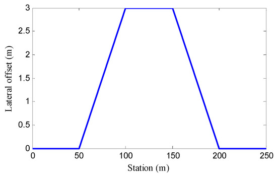
Figure 2.
Double lane changes maneuver.
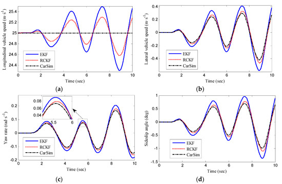
Figure 3.
Comparison of estimation effects in double lane changes maneuver: (a) Longitudinal vehicle speed; (b) lateral vehicle speed; (c) yaw rate; (d) sideslip angle.
In order to further quantitatively reflect the improvement effect of RCKF on estimation accuracy, the average error (AE) and root mean square error (RMSE) of the estimation results were used to represent the estimation effect of the proposed method (the same below). The computational formulas of AE and RMSE can be given by
where n is the sampling constant, xi represents the actual and estimated vehicle running states at the ith sampling time. The quantitative comparative analysis of the estimated results in the double lane change maneuver is shown in Table 2. As shown in Table 2, both the AE and RMSE of EKF are smaller than that of RCKF, indicating that RCKF improves the accuracy and stability of the overall estimation results. By evaluating the effect in improving estimation accuracy according to AE, one can find that, compared with EKF, the accuracy of RCKF in estimating longitudinal vehicle speed, lateral vehicle speed, yaw rate, and sideslip angle is improved by 0.21%, 15.83%, 4.37%, and 16.11%, respectively. Taking its average value as the overall estimation accuracy improvement ratio, the overall estimation accuracy is improved by 9.13%.
Table 2.
Quantitative analysis of estimation effects in double lane changes maneuver.
4.2. Case Study 2: Fishhook Maneuver
In order to further verify the estimation effect of the proposed method under complex conditions, the simulation of fishhook working conditions under low adhesion road conditions was carried out. In the simulation, the steering wheel angle is shown in Figure 4. The simulation conditions were specified as follows: The road adhesion coefficient was 0.6, the iterative step sizes of EKF and RCKF were 0.01 s, the initial state value was , the error covariance matrix is , the measurement noise covariance matrix was .
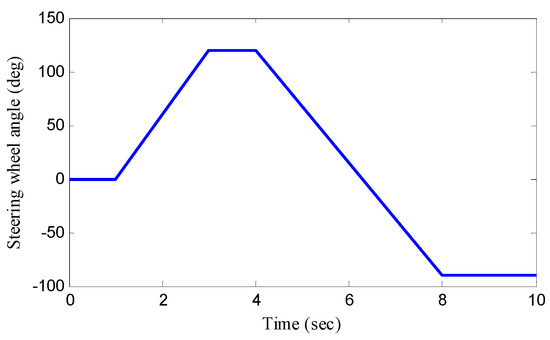
Figure 4.
Fishhook maneuver.
The simulation results are shown in Figure 5, in which Figure 5a–d represents the comparison results of the longitudinal vehicle speed, lateral vehicle speed, yaw rate, and vehicle sideslip angle, respectively. According to the local enlargement diagram in Figure 5a,c, it can be found that the results of RCKF in longitudinal vehicle speed and yaw rate estimation are better than that of EKF. From Figure 5b,d, it can be seen that compared with EKF, RCKF improves the estimation accuracy of lateral vehicle speed and sideslip angle obviously. Compared with the actual vehicle state output by CarSim, the estimation result of RCKF has some lag, which is mainly due to the larger amount of calculation of RCKF. Moreover, compared with the magnitude of lateral vehicle speed and sideslip angle, the estimation error caused by this delay is very small and within the allowable range. The simulation results in Figure 5 show that the proposed RCKF-based wheel-speed-coupling estimation method can still maintain accurate estimation performance in the case of drastic changes in vehicle driving state and severe driving conditions, and the anti-interference and reliability of the proposed method are verified. The values of AE and RMSE in the fishhook maneuver can be calculated out by Equations (37) and (38), similarly, and the calculation results are shown in Table 3. It can be found that the AE and RMSE of RCKF are smaller than that of EKF in the fishhook maneuver. Compared with EKF, the accuracy of RCKF in estimating longitudinal vehicle speed, lateral vehicle speed, yaw rate, and sideslip angle is improved by 0.53%, 14.69%, 4.06%, and 14.85%, respectively, and the overall estimation accuracy is improved by 8.53%. Thus, the estimation effect of the proposed method is further verified.
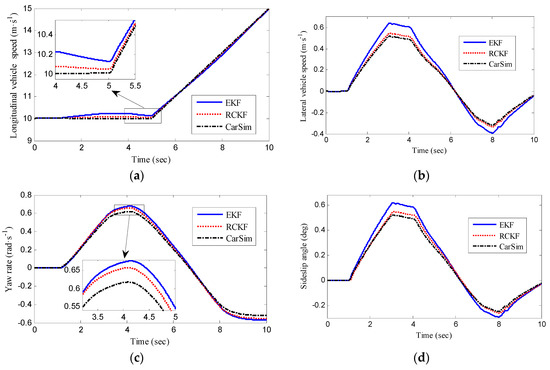
Figure 5.
Comparison of estimation effects in fishhook maneuver: (a) Longitudinal vehicle speed; (b) lateral vehicle speed; (c) yaw rate; (d) sideslip angle.
Table 3.
Quantitative analysis of estimation effects in the fishhook maneuver.
5. Experimental Verifications
In order to verify the real vehicle effect of the proposed estimation method, a modified intelligent vehicle was used to execute the road test. The overall control system architecture, vehicle signal transmission system, and vehicle refitting parameters of the refitted vehicle are described in detail in Reference 5. The refitted vehicle and experimental trajectory in the road test are shown in Figure 6. In Figure 6a, the vehicle speed cruising was regulated well by a speed controller, the front wheel steering angle was transformed from the measured hand steering wheel angle, the longitudinal vehicle speed and sideslip angle were measured by high-precision difference GPS, the yaw rate was obtained by an inertial measurement unit (IMU), and the four-wheel rotation speeds were acquired by the wheel speed sensor mounted on four wheels. All measurements of corresponding sensors were recorded by the host computer through CAN bus using CAN tools of Vehicle SPY 3.
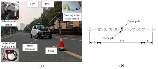
Figure 6.
Vehicle road test: (a) Refitted vehicle; (b) experimental trajectory.
In the experimental verification, the iterative step sizes of EKF and RCKF were 0.001 s, the initial state value was , the error covariance matrix was , the measurement noise covariance matrix was . The collected vehicle running states are shown in Figure 7, and the experimental verification results are shown in Figure 8 and Table 4. From Figure 8 and Table 4, it can be seen that RCKF can still maintain good estimation performance in practical applications, and the estimation accuracy of RCKF is significantly improved compared with EKF. By calculation, it can be found that, compared with EKF, the accuracy of RCKF in estimating longitudinal vehicle speed, lateral vehicle speed, yaw rate, and sideslip angle is improved by 4.22%, 15.38%, 8.36%, and 16.93%, respectively, and the overall estimation accuracy is improved by 11.22%.
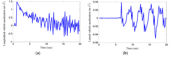
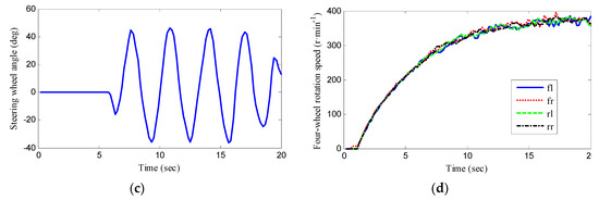
Figure 7.
Measured running states of vehicle road test: (a) Longitudinal vehicle acceleration; (b) lateral vehicle acceleration; (c) steering wheel angle; (d) four-wheel rotation speed.
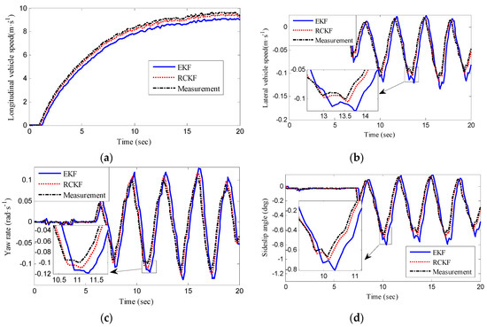
Figure 8.
Comparison of estimation effects in road test: (a) Longitudinal vehicle speed; (b) lateral vehicle speed; (c) yaw rate; (d) sideslip angle.
Table 4.
Quantitative analysis of estimation effects in road test.
6. Conclusions
In this work, a sideslip angle estimation method of an autonomous vehicle based on a robust cubature Kalman filter and wheel-speed coupling relationship is proposed, and the contributions of this paper can be summarized as follows: 1) Aiming at the problem of estimating sideslip angle of an intelligent vehicle, a three-degree-of-freedom vehicle dynamics model, tire model, and wheel-speed coupling model are established, and a method for estimating the vehicle sideslip angle is designed based on the robust cubature Kalman filter and wheel-speed coupling relationship; 2) an adaptive measurement-update solution is developed to improve the robustness and self-adaptability of estimation, and the wheel-speed coupling relationship is applied to the measurement update process of filter to improve the reliability of the estimation results. The simulation test based on the CarSim and Simulink co-simulation model and actual vehicle road test were carried out, and the estimation results of EKF were used to compare with RCKF; 3) the simulation and experimental results show that the proposed estimation method can achieve a more accurate vehicle state estimation result than EKF, and has better reliability and real-time tracking capability. Compared with EKF, the overall estimation accuracy in a real vehicle application is improved by 11.22%.
Author Contributions
Conceptualization, T.C., L.C. and X.X.; methodology, T.C. and X.X.; software, T.C. and X.X.; validation, T.C. and X.X.; formal analysis, Y.C., H.J. and X.S.; investigation, Y.C. and X.S.; resources, L.C. and X.X.; data curation, T.C. and X.X.; writing—original draft preparation, T.C.; writing—review and editing, T.C.; visualization, T.C.; supervision, L.C. and X.X.; project administration, L.C., X.X. and T.C.; funding acquisition, L.C. and X.X.
Funding
This research was supported by the National Natural Science Foundation of China (Grant No. U1564201, U1664258, and 51875255), the National Key Research and Development Program of China (Grant No. 2017YFB0102603), the Six Talent Peaks Project of Jiangsu Province (Grant No. 2018-TD-GDZB-022), the Key Project for the Development of Strategic Emerging Industries of Jiangsu Province (2016-1094, 2015-1084), the Primary Research & Development Plan of Jiangsu Province (Grant No. BE2016149), the Postgraduate Scientific Research Innovation Program of Jiangsu Province (Grant No. SJKY19_2536).
Conflicts of Interest
The authors declare that there is no conflict of interest.
References
- Chen, T.; Chen, L.; Cai, Y.; Xu, X. Estimation of vehicle sideslip angle via pseudo-multisensor information fusion method. Metrol. Meas. Syst. 2018, 25, 499–516. [Google Scholar]
- Zhang, H.; Wang, J. Vehicle lateral dynamics control through AFS/DYC and robust gain-scheduling approach. IEEE Trans. Veh. Technol. 2016, 65, 489–494. [Google Scholar] [CrossRef]
- Zhang, L.; Zhao, Z.; Chai, J.; Kan, Z. Risk Identification and Analysis for PPP Projects of Electric Vehicle Charging Infrastructure Based on 2-Tuple and the DEMATEL Model. World Electr. Veh. J. 2019, 10, 4. [Google Scholar] [CrossRef]
- Qiu, H.; Dong, Z.; Lei, Z. Simulation and experiment of integration control of ARS and DYC for electrical vehicle with four wheel independent drive. J. Jiangsu Univ. Nat. Sci. Ed. 2016, 37, 268–276. [Google Scholar]
- Xu, X.; Chen, T.; Chen, L.; Wang, W. Longitudinal force estimation for motorized wheels driving electric vehicle based on improved closed-loop subspace identification. J. Jiangsu Univ. Nat. Sci Ed. 2016, 37, 650–656. [Google Scholar]
- Chen, Y.; Wang, J. Adaptive vehicle speed control with input injections for longitudinal motion independent road frictional condition estimation. IEEE Trans. Veh. Technol. 2011, 60, 839–848. [Google Scholar] [CrossRef]
- Shen, K.; Selezneva, M.; Neusypin, K.; Proletarsky, A. Novel variable structure measurement with intelligent components flight vehicles. Metrol. Meas. Syst. 2017, 24, 347–356. [Google Scholar] [CrossRef]
- Chen, T.; Xu, X.; Li, Y.; Wang, W.; Chen, L. Speed-dependent coordinated control of differential and assisted steering for in-wheel motor driven electric vehicles. Proc. Inst. Mech. E Part D J. Automob. Eng. 2018, 232, 1206–1220. [Google Scholar] [CrossRef]
- Yang, L.; Tang, Y.; Tang, L.; Wu, C. Brushless DC motor drive characteristics and system for reel-type irrigator. J. Drain. Irrig. Mach. Eng. 2018, 36, 690–695. [Google Scholar]
- Gu, Z.; Yuan, S.; Tang, L.; Tang, Y. Intelligent solar drive control system of hose reel irrigator. J. Drain. Irrig. Mach. Eng. 2018, 36, 969–974. [Google Scholar]
- Iora, P.; Tribioli, L. Effect of ambient temperature on electric vehicles’ energy consumption and range: Model definition and sensitivity analysis based on nissan leaf data. World Electr. Veh. J. 2019, 10, 2. [Google Scholar] [CrossRef]
- Jiang, H.; Li, A.; Ma, S.; Chen, L. Design and performance analysis of airflow energy recovery device of electric vehicle. J. Jiangsu Univ. Nat. Sci. Ed. 2017, 38, 125–132. [Google Scholar]
- Chen, T.; Chen, L.; Xu, X.; Cai, Y.; Sun, X. Simultaneous path following and lateral stability control of 4WD-4WS autonomous electric vehicles with actuator saturation. Adv. Eng. Softw. 2019, 128, 46–54. [Google Scholar] [CrossRef]
- Anil, K.; Matteo, C.; Edward, H. Vehicle sideslip estimator using load sensing bearings. Control Eng. Pract. 2016, 54, 46–57. [Google Scholar]
- Wang, J.; Li, J. Hierarchical coordinated control method of in-wheel motor drive electric vehicle based on energy optimization. World Electr. Veh. J. 2019, 10, 15. [Google Scholar] [CrossRef]
- Chen, T.; Xu, X.; Chen, L.; Jiang, H.; Cai, Y. Estimation of longitudinal force, lateral vehicle speed and yaw rate for four-wheel independent driven electric vehicles. Mech. Syst. Signal Process. 2018, 101, 377–388. [Google Scholar] [CrossRef]
- Chen, T.; Chen, L.; Cai, Y.; Xu, X. Robust sideslip angle observer with regional stability constraint for an uncertain singular intelligent vehicle system. IET Control Theory Appl. 2018, 12, 1802–1811. [Google Scholar] [CrossRef]
- Fan, Y.; Huang, X.; Li, J.; Wang, T.; Du, F. Stability analysis on light weight and small size watering cart for dual purpose of both sprinkling irrigation and hose irrigation. J. Drain. Irrig. Mach. Eng. 2010, 28, 256–259. [Google Scholar]
- Li, L.; Jia, G.; Ran, X.; Song, J.; Wu, K. Avariable structure extended Kalman filter for vehicle side slip angle estimation on a low friction road. Veh. Syst. Dyn. 2014, 52, 280–308. [Google Scholar] [CrossRef]
- Martin, H.; Johannes, E.; Manfred, P.; Manuel, H. Vehicle side-slip angle estimation on a banked and low-friction road. Proc. Inst. Mech. E Part D J. Automob. Eng. 2017. [Google Scholar] [CrossRef]
- Wang, R.R.; Zhang, H.; Wang, J. Linear parameter-varying controller design for four-wheel independently actuated electric ground vehicles with active steering systems. IEEE Trans. Control Syst. Technol. 2014, 22, 1281–1296. [Google Scholar]
- Zhang, H.; Wang, J. Active steering actuator fault detection for an automatically-steered electric ground vehicle. IEEE Trans. Veh. Technol. 2017, 66, 3685–3702. [Google Scholar] [CrossRef]
- Zhang, H.; Huang, X.; Wang, J. Robust energy-to-peak sideslip angle estimation with applications to ground vehicles. Mechatronics 2015, 30, 338–347. [Google Scholar] [CrossRef]
- Yoon, J.; Peng, H. Robust vehicle sideslip angle estimation through a disturbance rejection filter that integrates a magnetometer with GPS. IEEE Trans. Intell. Transp. Syst. 2014, 15, 191–204. [Google Scholar] [CrossRef]
- Liu, W.; He, H.; Sun, F. Vehicle state estimation based on minimum model error criterion combining with extended Kalman filter. J. Frankl. Inst. 2016, 353, 834–856. [Google Scholar] [CrossRef]
- Zhang, H.; Zhang, G.; Wang, J. Sideslip angle estimation of an electric ground vehicle via finite-frequency H∞ approach. IEEE Trans. Transp. Electr. 2016, 2, 200–209. [Google Scholar] [CrossRef]
- Cheli, F.; Braghin, F.; Brusarosco, M.; Mancosu, F.; Sabbioni, E. Design and testing of an innovative measurement device for tyre-road contact forces. Mech. Syst. Signal Process. 2011, 25, 1956–1972. [Google Scholar] [CrossRef]
- Zhu, H.; Li, L.; Jin, M.; Li, H.; Song, J. Real-time yaw rate prediction based on a non-linear model and feedback compensation for vehicle dynamics control. Proc. Inst. Mech. Eng. D J. Automob. Eng. 2013, 227, 1431–1445. [Google Scholar] [CrossRef]
- Rath, J.; Veluvolu, K.; Defoort, M.; Soh, Y. Higher-order sliding mode observer for estimation of tyre friction in ground vehicles. IET Control Theory Appl. 2014, 8, 399–408. [Google Scholar] [CrossRef]
- Leung, K.; Whildborne, J.; Purdy, D.; Barber, P. Road vehicle state estimation using low-cost GPS/INS. Mech. Syst. Signal Process. 2011, 25, 1988–2004. [Google Scholar] [CrossRef]
- Nam, K.; Fujimoto, H.; Hori, Y. Lateral stability control of in-wheel-motor-driven electric vehicles based on sideslip angle estimation using lateral tire force sensors. IEEE Trans. Veh. Technol. 2012, 61, 1972–1985. [Google Scholar]
- Chen, L.; Bian, M.; Luo, Y.; Li, K. Real-time identification of the tyre-road friction coefficient using an unscented Kalman filter and mean-square-error-weighted fusion. Proc. Inst. Mech. Eng. D J. Automob. Eng. 2015, 230, 788–802. [Google Scholar] [CrossRef]
- Chen, T.; Chen, L.; Xu, X.; Cai, Y.; Jiang, H.; Sun, X. Estimation of longitudinal force and sideslip angle for intelligent four-wheel independent drive electric vehicles by observer iteration and information fusion. Sensors 2018, 2018, 1268. [Google Scholar] [CrossRef]
- Li, X.; Song, X.; Chan, C. Reliable vehicle sideslip angle fusion estimation using low-cost sensors. Measurement 2014, 51, 241–258. [Google Scholar] [CrossRef]
- Li, X.; Chan, C.; Wang, Y. A reliable fusion methodology for simultaneous estimation of vehicle sideslip and yaw angles. IEEE Trans. Veh. Technol. 2016, 65, 4440–4458. [Google Scholar] [CrossRef]
- Boada, B.; Boada, M.; Diaz, V. Vehicle side slip angle measurement based on sensor data fusion using an integrated ANFIS and an Unscented Kalman Filter algorithm. Mech. Syst. Signal Process. 2016, 72, 832–845. [Google Scholar] [CrossRef]
- Jin, X.; Yin, G. Estimation of lateral tire-road forces and sideslip angle for electric vehicles using interacting multiple model filter approach. J. Frankl. Inst 2015, 352, 686–707. [Google Scholar] [CrossRef]
- Yoon, J.H.; Li, S.E.; Ahn, C. Estimation of vehicle sideslip angle and tire-road friction coefficient based on magnetometer with GPS. Int. J. Automot. Technol. 2016, 17, 427–435. [Google Scholar] [CrossRef]
- Liu, Y.; Li, T.; Yang, Y.; Ji, X.; Wu, J. Estimation of tire-road friction coefficient based on combined APF-IEKF and iteration algorithm. Mech. Syst. Signal Process. 2017, 88, 25–35. [Google Scholar] [CrossRef]
- Cheng, S.; Li, L.; Chen, J. Fusion algorithm design based on adaptive SCKF and integral correction for side-slip angle observation. IEEE Trans. Ind. Electron. 2018, 65, 5754–5763. [Google Scholar] [CrossRef]
- Nam, K.; Oh, S.; Fujimoto, H.; Hori, Y. Estimation of sideslip angle and roll angles of electric vehicles using lateral tire force sensors through RLS and Kalman filter approaches. IEEE Trans. Ind. Electron. 2013, 60, 988–1000. [Google Scholar] [CrossRef]


© 2019 by the authors. Licensee MDPI, Basel, Switzerland. This article is an open access article distributed under the terms and conditions of the Creative Commons Attribution (CC BY) license (http://creativecommons.org/licenses/by/4.0/).