


MCSNet: A Radio Frequency Interference Suppression Network for Spaceborne SAR Images via Multi-Dimensional Feature Transform
Abstract
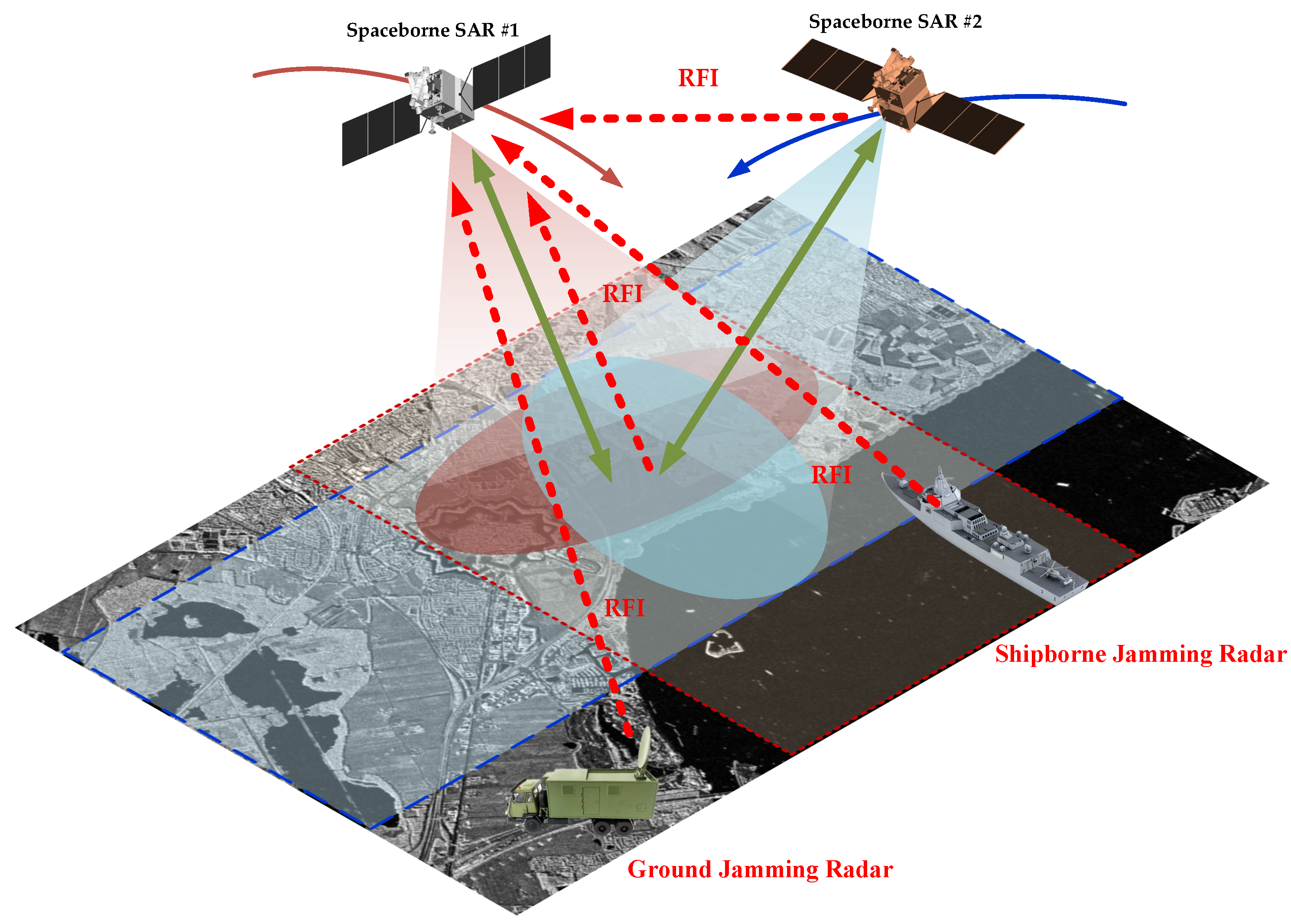
1. Introduction
- 1.
- A strategy for SAR images RFI suppression across multi-dimensions and multi-channel.
- 2.
- A module applied to the global structure, with functions for extracting deep image features and calibrating the mapping of feature maps; A novel method with a supervised mechanism for calibrating image features and maintaining the scattering characteristics of SAR images with fine detail.
- 3.
- The corresponding results show that MCSNet owns the characteristic functionality of RFI suppression.
2. SAR Image Model and Equations
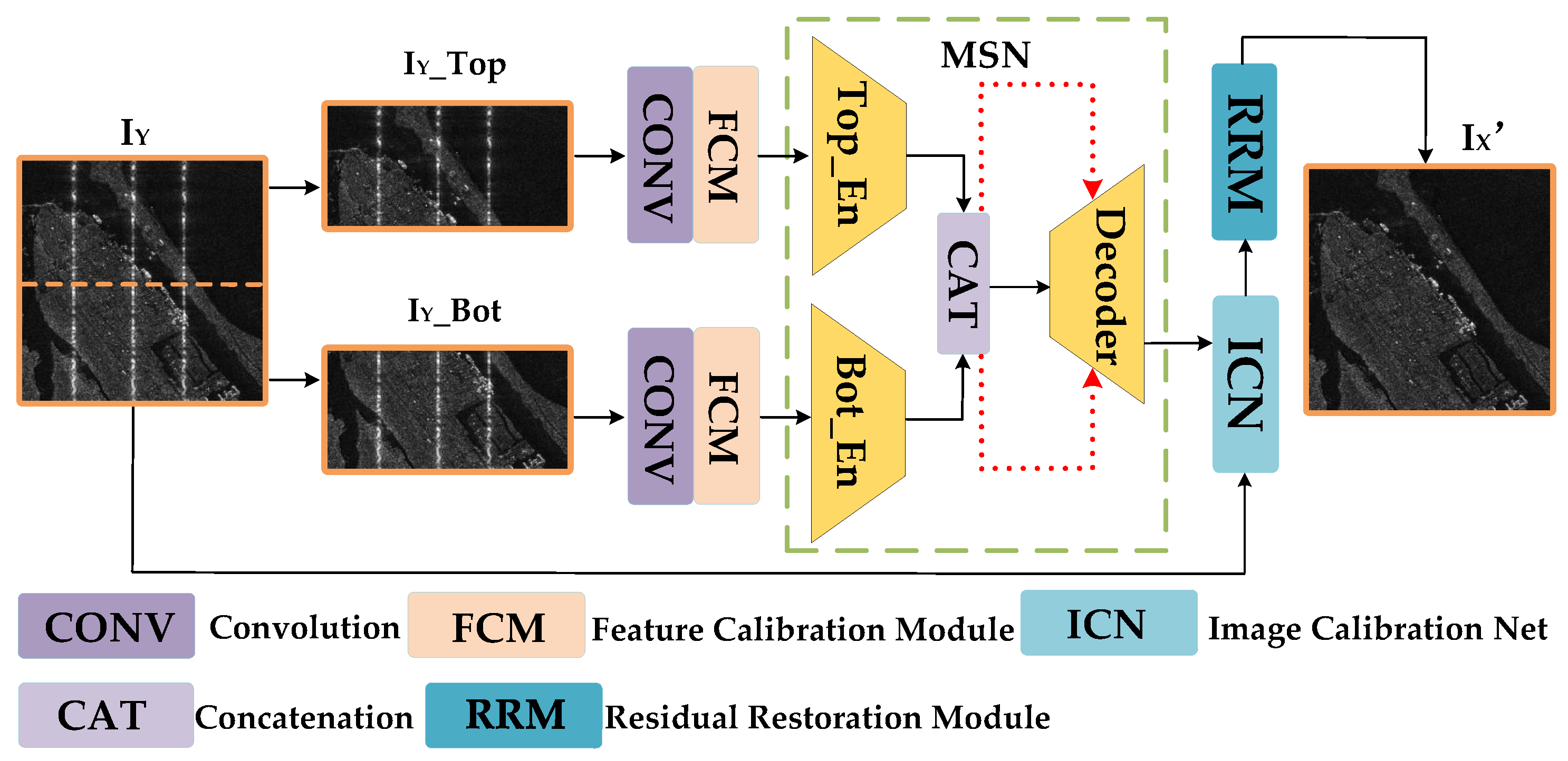
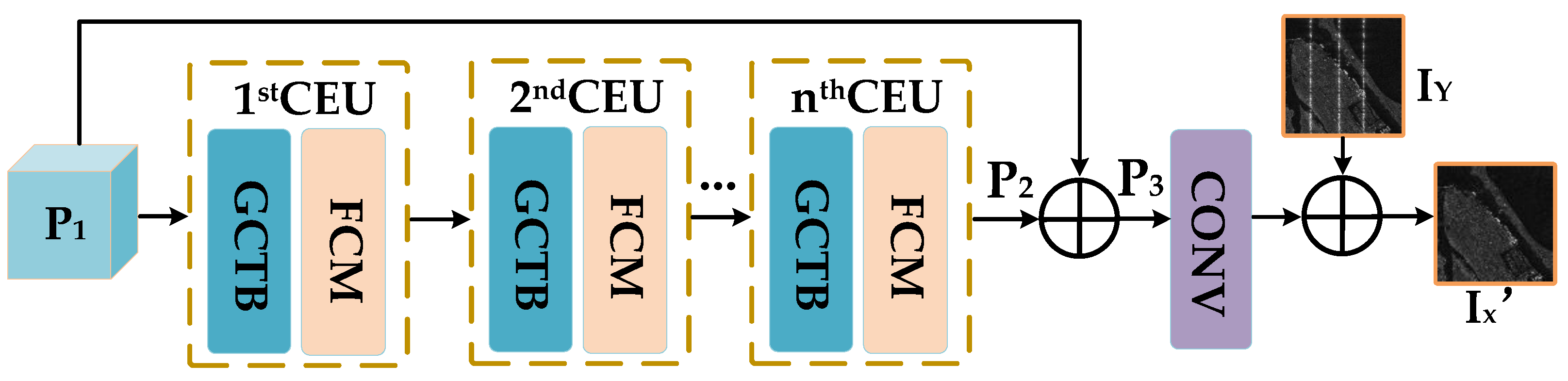
3. The Proposed Method
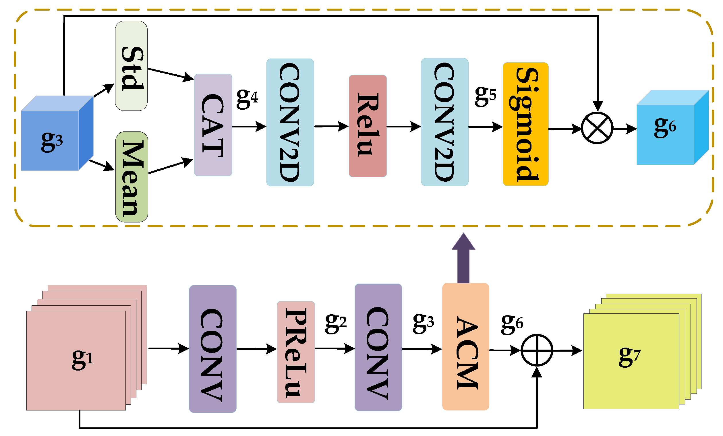
3.1. FCM
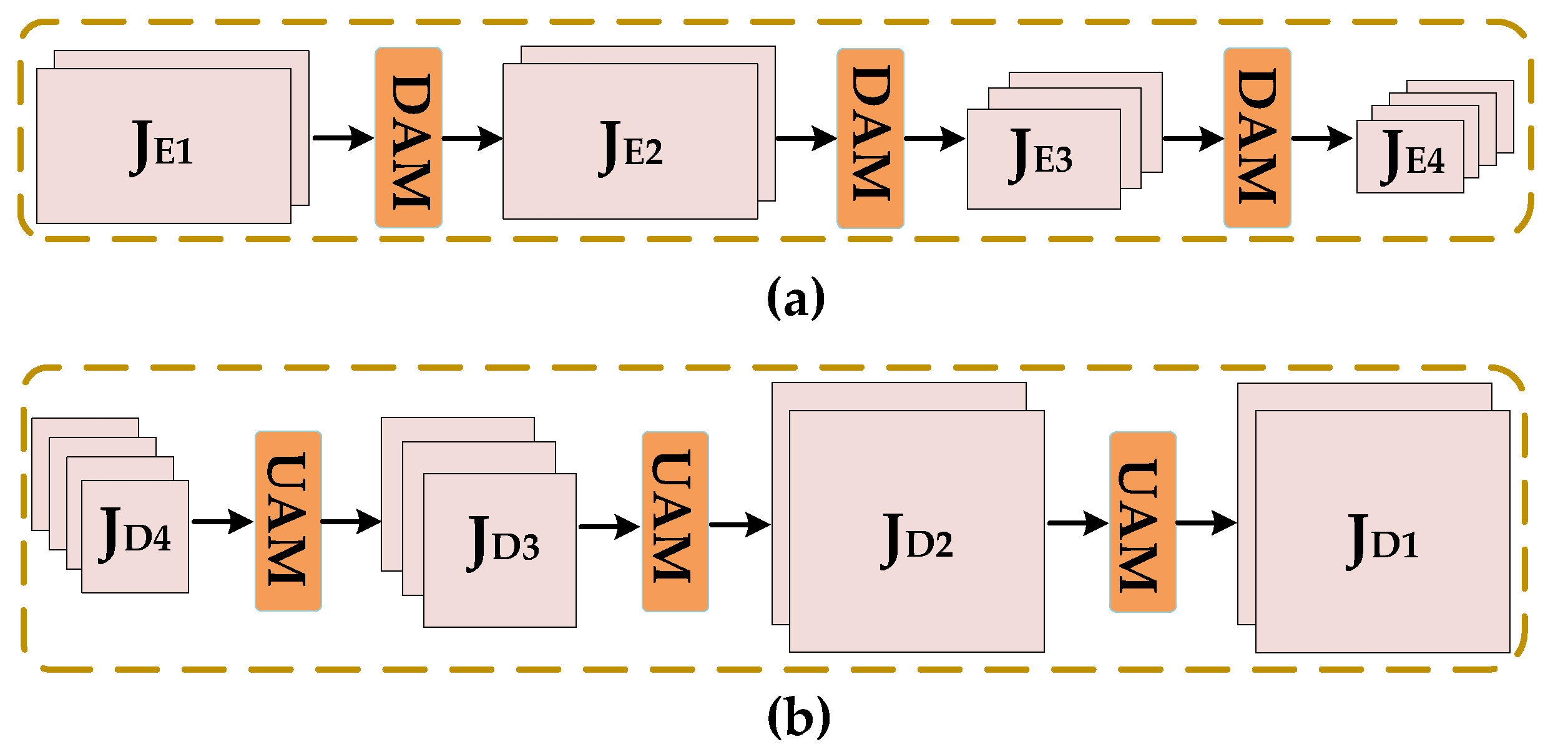
3.2. MSN
3.3. ICN
3.4. RRM
4. Experiments and Results
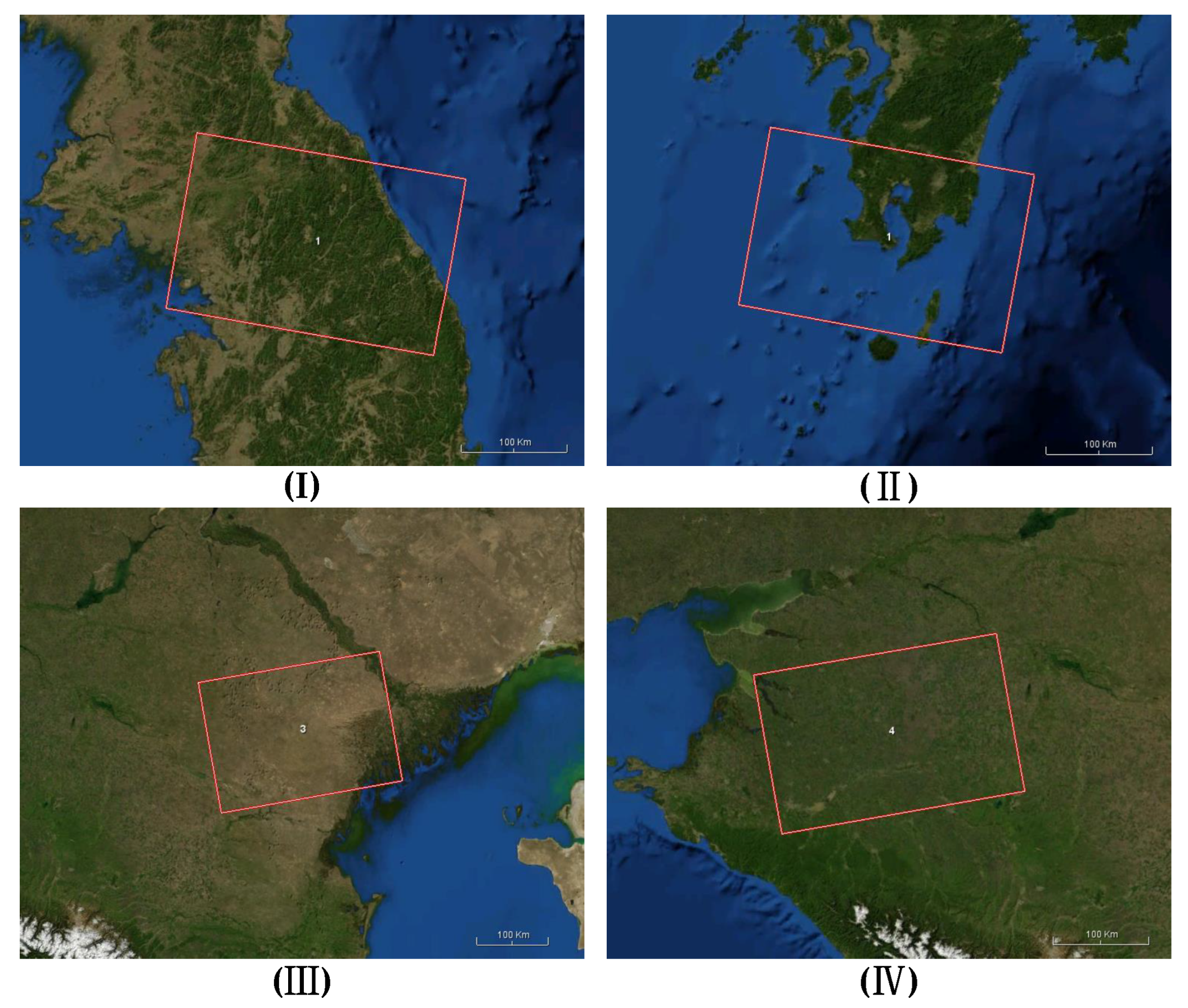
4.1. Dataset
4.2. Loss Function
4.3. Assessment Indicators
4.4. Simulation Data Results
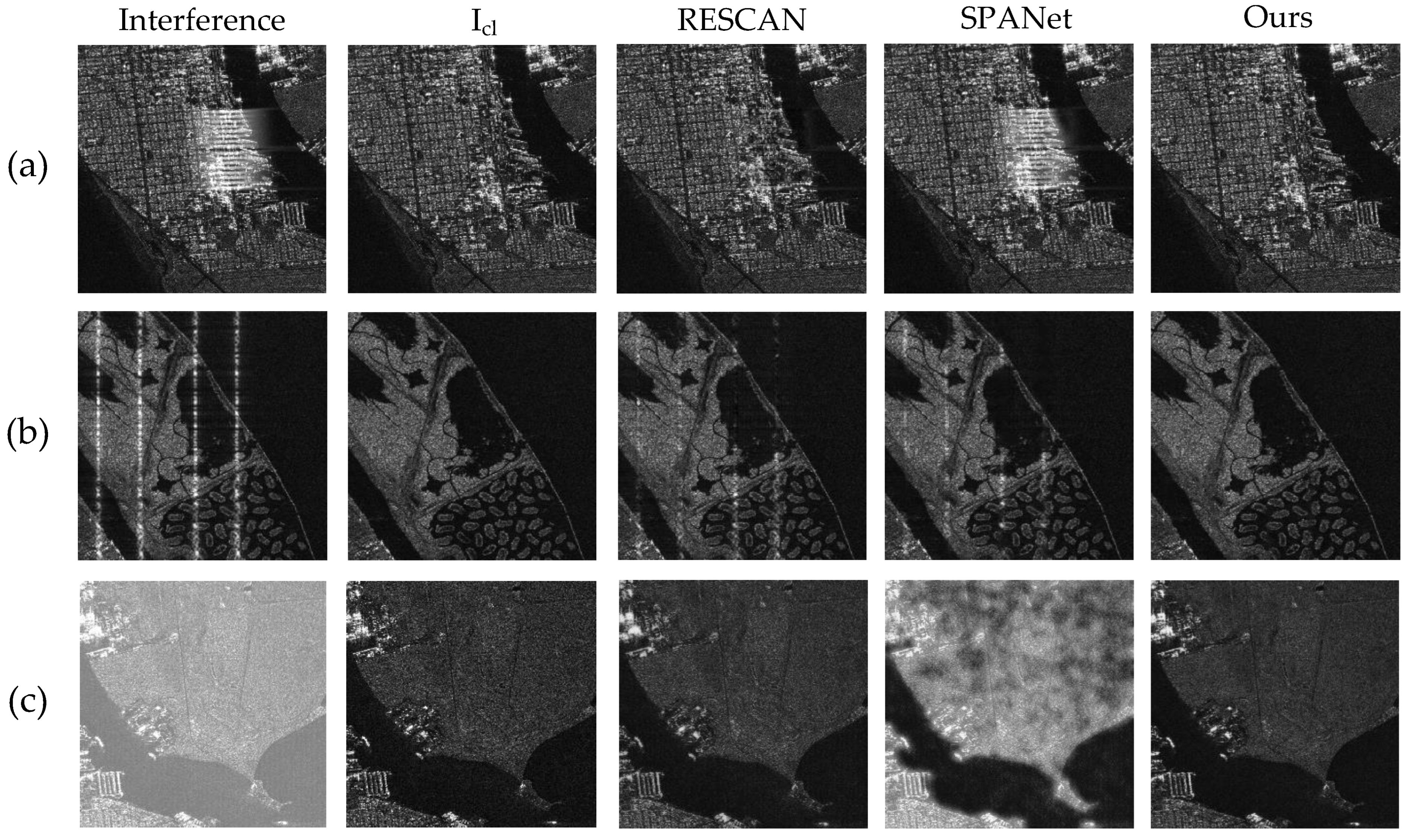
4.4.1. Visual Results
4.4.2. Closeness between Results and Clean Images
4.4.3. Image Quality
4.5. Measured Data Results
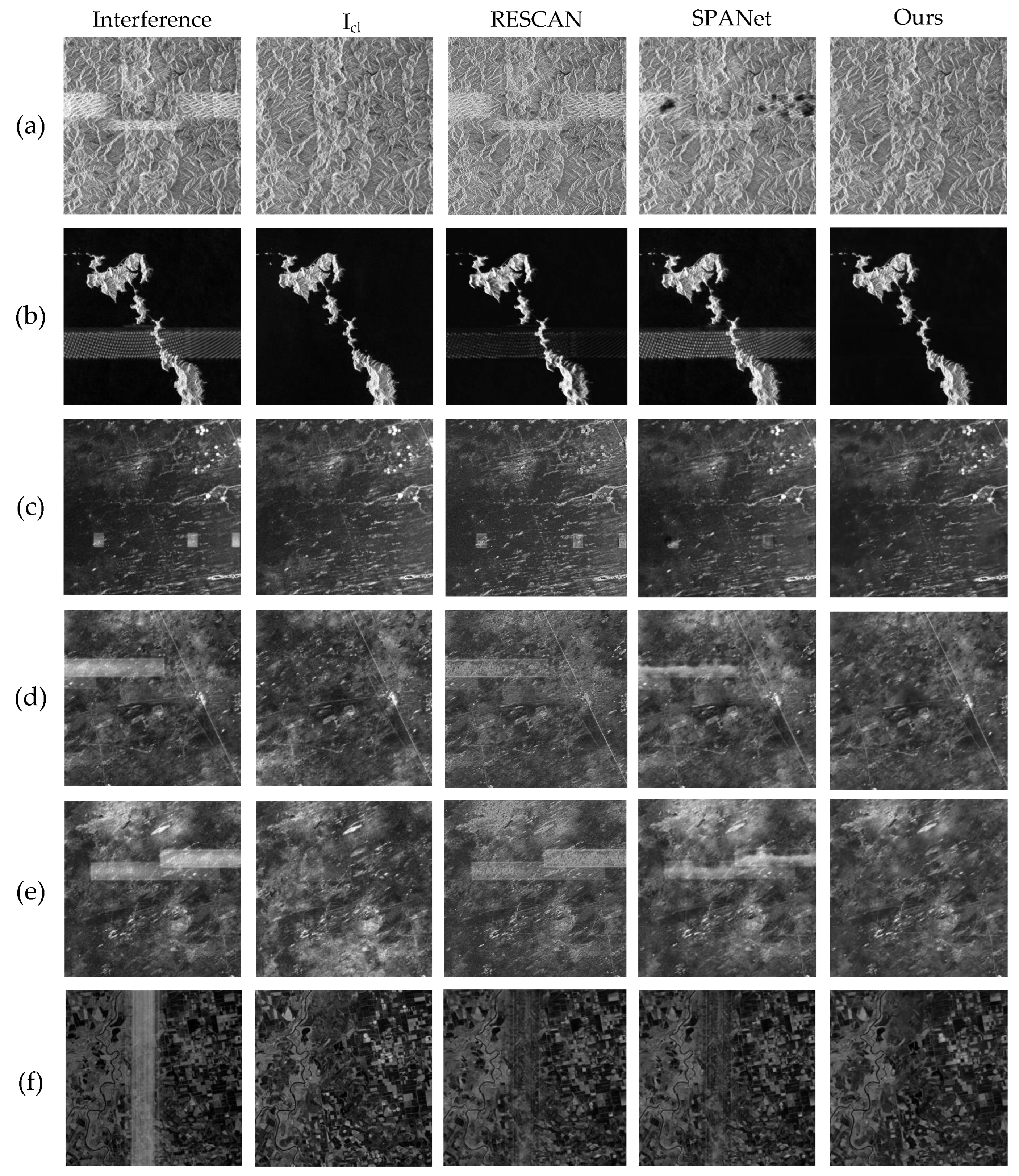
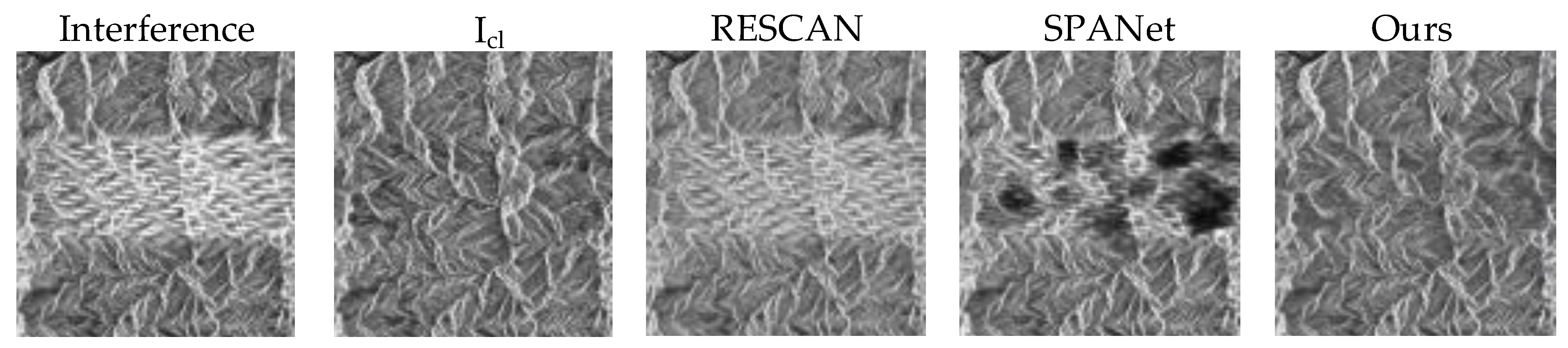
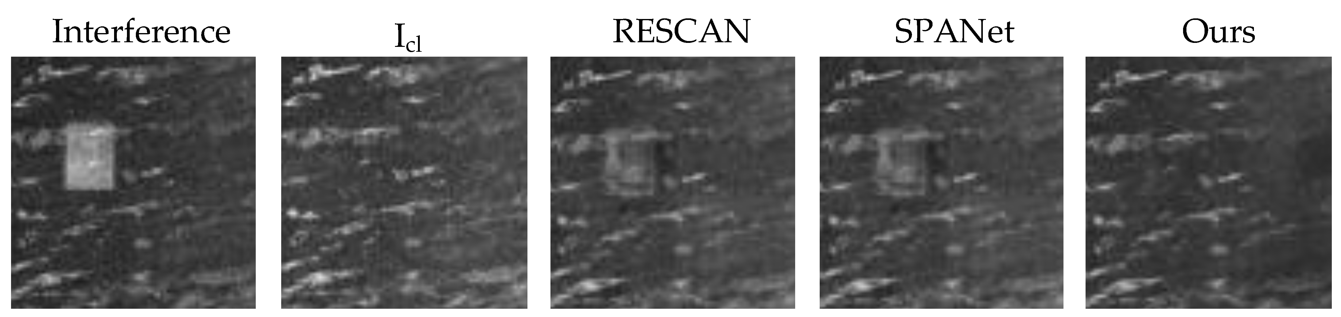
4.5.1. Visual Results


4.5.2. Closeness between Results and Clean Images
4.5.3. Image Quality
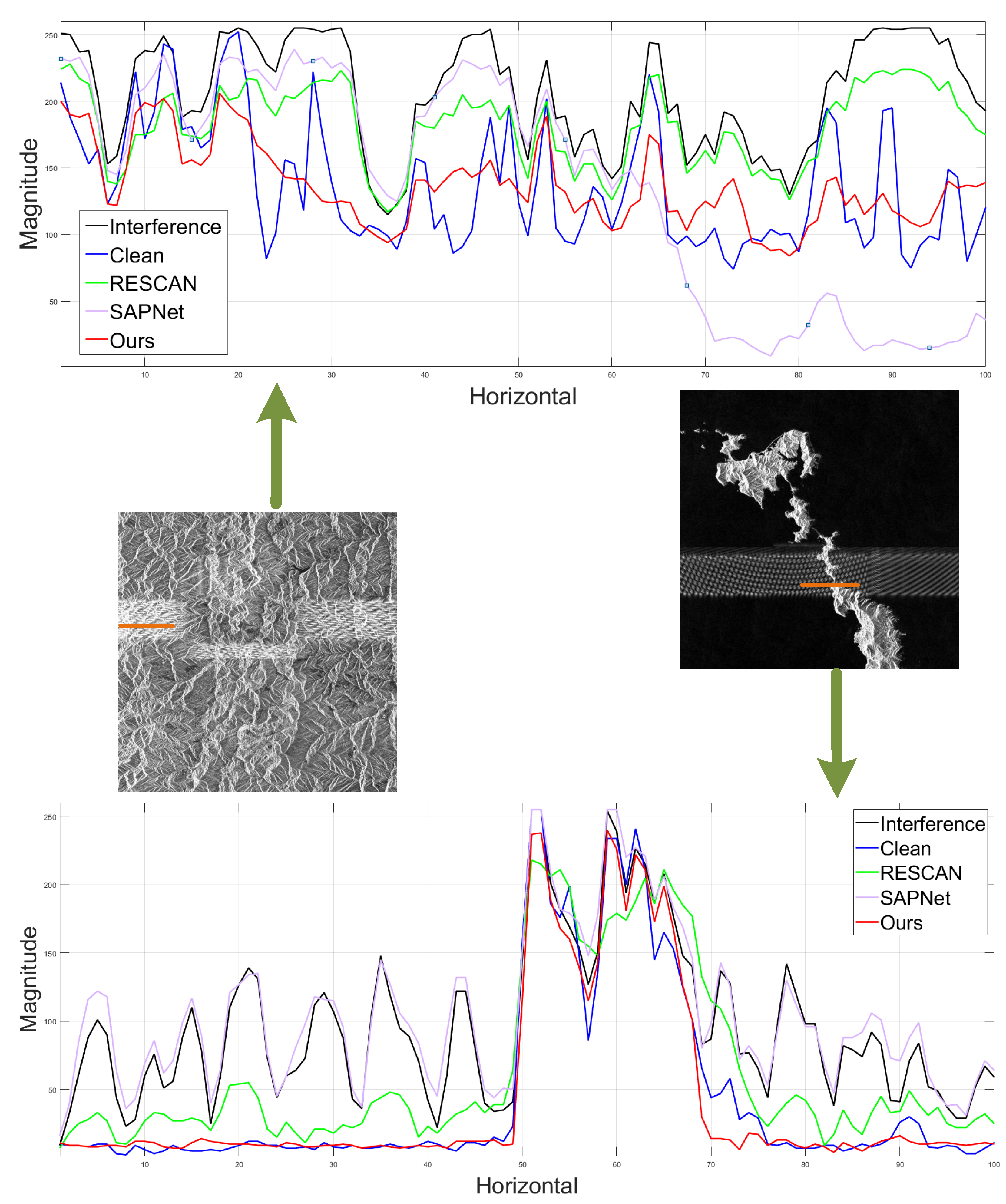
4.5.4. Comparisons of Scattering Characteristics
5. Conclusions
6. Discussion
Author Contributions
Funding
Data Availability Statement
Acknowledgments
Conflicts of Interest
References
- Zhou, Z.; Wei, S.; Zhang, H.; Shen, R.; Wang, M.; Shi, J.; Zhang, X. SAF-3DNet: Unsupervised AMP-Inspired Network for 3-D MMW SAR Imaging and Autofocusing. IEEE Trans. Geosci. Remote Sens. 2022, 60, 5234915. [Google Scholar] [CrossRef]
- Wei, S.; Zeng, X.; Zhang, H.; Zhou, Z.; Shi, J.; Zhang, X. LFG-Net: Low-Level Feature Guided Network for Precise Ship Instance Segmentation in SAR Images. IEEE Trans. Geosci. Remote Sens. 2022, 60, 5231017. [Google Scholar] [CrossRef]
- Lao, D.; Zhu, B.; Yu, S.; Guo, Y. An Improved SAR Imaging Algorithm Based on a Two-Dimension-Separated Algorithm. In Proceedings of the 2018 China International SAR Symposium (CISS), Shanghai, China, 10–12 October 2018; pp. 1–3. [Google Scholar] [CrossRef]
- Zeng, X.; Wei, S.; Shi, J.; Zhang, X. A Lightweight Adaptive RoI Extraction Network for Precise Aerial Image Instance Segmentation. IEEE Trans. Instrum. Meas. 2021, 70, 5018617. [Google Scholar] [CrossRef]
- Liu, G.; Liu, B.; Zheng, G.; Li, X. Environment Monitoring of Shanghai Nanhui Intertidal Zone with Dual-Polarimetric SAR Data Based on Deep Learning. IEEE Trans. Geosci. Remote Sens. 2022, 60, 4208918. [Google Scholar] [CrossRef]
- AlAli, Z.T.; Alabady, S.A. A survey of disaster management and SAR operations using sensors and supporting techniques. Int. J. Disaster Risk Reduct. 2022, 82, 103295. [Google Scholar] [CrossRef]
- Salvia, M.; Franco, M.; Grings, F.; Perna, P.; Martino, R.; Karszenbaum, H.; Ferrazzoli, P. Estimating Flow Resistance of Wetlands Using SAR Images and Interaction Models. Remote Sens. 2009, 1, 992–1008. [Google Scholar] [CrossRef]
- Li, N.; Lv, Z.; Guo, Z. Observation and Mitigation of Mutual RFI Between SAR Satellites: A Case Study Between Chinese GaoFen-3 and European Sentinel-1A. IEEE Trans. Geosci. Remote Sens. 2022, 60, 5112819. [Google Scholar] [CrossRef]
- Xu, W.; Xing, W.; Fang, C.; Huang, P.; Tan, W. RFI Suppression Based on Linear Prediction in Synthetic Aperture Radar Data. IEEE Geosci. Remote Sens. Lett. 2021, 18, 2127–2131. [Google Scholar] [CrossRef]
- Chen, Z.; Zhou, S.; Wang, X.; Huang, Y.; Wan, J.; Li, D.; Tan, X. Single Range Data-Based Clutter Suppression Method for Multichannel SAR. IEEE Geosci. Remote Sens. Lett. 2022, 19, 4012905. [Google Scholar] [CrossRef]
- Li, N.; Zhang, H.; Lv, Z.; Min, L.; Guo, Z. Simultaneous Screening and Detection of RFI From Massive SAR Images: A Case Study on European Sentinel-1. IEEE Trans. Geosci. Remote Sens. 2022, 60, 5231917. [Google Scholar] [CrossRef]
- Wei, S.; Zhang, H.; Zeng, X.; Zhou, Z.; Shi, J.; Zhang, X. CARNet: An effective method for SAR image interference suppression. Int. J. Appl. Earth Obs. Geoinf. 2022, 114, 103019. [Google Scholar] [CrossRef]
- Tang, Z.; Deng, Y.; Zheng, H. RFI Suppression for SAR via a Dictionary-Based Nonconvex Low-Rank Minimization Framework and Its Adaptive Implementation. Remote Sens. 2022, 14, 678. [Google Scholar] [CrossRef]
- Lord, R.T.; Inggs, M.R. Efficient RFI suppression in SAR using LMS adaptive filter integrated with range/Doppler algorithm. Electron. Lett. IEE 1999, 35, 629. [Google Scholar] [CrossRef]
- Li, N.; Lv, Z.; Guo, Z.; Zhao, J. Time-Domain Notch Filtering Method for Pulse RFI Mitigation in Synthetic Aperture Radar. IEEE Geosci. Remote Sens. Lett. 2022, 19, 4013805. [Google Scholar] [CrossRef]
- Zhou, F.; Wu, R.; Xing, M.; Bao, Z. Eigensubspace-Based Filtering with Application in Narrow-Band Interference Suppression for SAR. IEEE Geosci. Remote Sens. Lett. 2007, 4, 75–79. [Google Scholar] [CrossRef]
- Chang, W.; Li, J.; Li, X. The Effect of Notch Filter on RFI Suppression. Wirel. Sens. Netw. 2009, 1, 196–205. [Google Scholar] [CrossRef]
- Wu, P.; Yang, L.; Zhang, Y.S.; Dong, Z.; Wang, M.; Du, S. A modified notch filter for suppressing radio-frequency-interference in P-band SAR data. In Proceedings of the 2016 IEEE International Geoscience and Remote Sensing Symposium (IGARSS), Beijing, China, 10–15 July 2016; pp. 4988–4991. [Google Scholar] [CrossRef]
- Xu, W.; Xing, W.; Fang, C.; Huang, P.; Tan, W.; Gao, Z. RFI Suppression for SAR Systems Based on Removed Spectrum Iterative Adaptive Approach. Remote Sens. 2020, 12, 3520. [Google Scholar] [CrossRef]
- Feng, J.; Zheng, H.; Deng, Y.; Gao, D. Application of Subband Spectral Cancellation for SAR Narrow-Band Interference Suppression. IEEE Geosci. Remote Sens. Lett. 2012, 9, 190–193. [Google Scholar] [CrossRef]
- Liu, H.; Li, D.; Zhou, Y.; Truong, T.K. Joint Wideband Interference Suppression and SAR Signal Recovery Based on Sparse Representations. IEEE Geosci. Remote Sens. Lett. 2017, 14, 1542–1546. [Google Scholar] [CrossRef]
- Lyu, Q.; Han, B.; Li, G.; Sun, W.; Pan, Z.; Hong, W.; Hu, Y. SAR Interference Suppression Algorithm Based on Low-Rank and Sparse Matrix Decomposition in Time–Frequency Domain. IEEE Geosci. Remote Sens. Lett. 2022, 19, 4008305. [Google Scholar] [CrossRef]
- Huang, Y.; Liao, G.; Zhang, Z.; Xiang, Y.; Li, J.; Nehorai, A. Fast Narrowband RFI Suppression Algorithms for SAR Systems via Matrix-Factorization Techniques. IEEE Trans. Geosci. Remote Sens. 2019, 57, 250–262. [Google Scholar] [CrossRef]
- Yang, H.; Chen, C.; Chen, S.; Xi, F.; Liu, Z. SAR RFI Suppression for Extended Scene Using Interferometric Data via Joint Low-Rank and Sparse Optimization. IEEE Geosci. Remote Sens. Lett. 2021, 18, 1976–1980. [Google Scholar] [CrossRef]
- Fang, J.; Hu, S.; Ma, X. A Boosting SAR Image Despeckling Method Based on Non-Local Weighted Group Low-Rank Representation. Sensors 2018, 18, 3448. [Google Scholar] [CrossRef] [PubMed]
- Zhou, F.; Xing, M.; Bai, X.; Sun, G.; Bao, Z. Narrow-Band Interference Suppression for SAR Based on Complex Empirical Mode Decomposition. IEEE Geosci. Remote Sens. Lett. 2009, 6, 423–427. [Google Scholar] [CrossRef]
- Lu, X.; Su, W.; Yang, J.; Gu, H.; Zhang, H.; Yu, W.; Yeo, T.S. Radio Frequency Interference Suppression for SAR via Block Sparse Bayesian Learning. IEEE J. Sel. Top. Appl. Earth Obs. Remote Sens. 2018, 11, 4835–4847. [Google Scholar] [CrossRef]
- Liu, H.; Li, D. RFI Suppression Based on Sparse Frequency Estimation for SAR Imaging. IEEE Geosci. Remote Sens. Lett. 2016, 13, 63–67. [Google Scholar] [CrossRef]
- Wang, M.; Wei, S.; Zhou, Z.; Shi, J.; Zhang, X. Efficient ADMM Framework Based on Functional Measurement Model for mmW 3-D SAR Imaging. IEEE Trans. Geosci. Remote Sens. 2022, 60, 5226417. [Google Scholar] [CrossRef]
- Fan, W.; Zhou, F.; Tao, M.; Bai, X.; Rong, P.; Yang, S.; Tian, T. Interference Mitigation for Synthetic Aperture Radar Based on Deep Residual Network. Remote Sens. 2019, 11, 1654. [Google Scholar] [CrossRef]
- Shen, J.; Han, B.; Pan, Z.; Hu, Y.; Hong, W.; Ding, C. Radio Frequency Interference Suppression in SAR System Using Prior-Induced Deep Neural Network. In Proceedings of the IGARSS 2022—2022 IEEE International Geoscience and Remote Sensing Symposium, Kuala Lumpur, Malaysia, 4–7 November 2022; pp. 943–946. [Google Scholar] [CrossRef]
- Li, X.; Wu, J.; Lin, Z.; Liu, H.; Zha, H. Recurrent squeeze-and-excitation context aggregation net for single image deraining. In Proceedings of the European Conference on Computer Vision (ECCV), Munich, Germany, 8–14 September 2018; pp. 254–269. [Google Scholar]
- Wang, T.; Yang, X.; Xu, K.; Chen, S.; Zhang, Q.; Lau, R.W. Spatial attentive single-image deraining with a high quality real rain dataset. In Proceedings of the IEEE/CVF Conference on Computer Vision and Pattern Recognition, Long Beach, CA, USA, 15–20 June 2019; pp. 12270–12279. [Google Scholar]
- Liu, Z.; Lai, R.; Guan, J. Spatial and Transform Domain CNN for SAR Image Despeckling. IEEE Geosci. Remote Sens. Lett. 2022, 19, 4002005. [Google Scholar] [CrossRef]
- Xiong, K.; Zhao, G.; Wang, Y.; Shi, G.; Chen, S. Lq-SPB-Net: A Real-Time Deep Network for SAR Imaging and Despeckling. IEEE Trans. Geosci. Remote Sens. 2022, 60, 5209721. [Google Scholar] [CrossRef]
- Su, J.; Tao, H.; Tao, M.; Wang, L.; Xie, J. Narrow-Band Interference Suppression via RPCA-Based Signal Separation in Time–Frequency Domain. IEEE J. Sel. Top. Appl. Earth Obs. Remote Sens. 2017, 10, 5016–5025. [Google Scholar] [CrossRef]
- Tao, M.; Su, J.; Huang, Y.; Wang, L. Mitigation of Radio Frequency Interference in Synthetic Aperture Radar Data: Current Status and Future Trends. Remote Sens. 2019, 11, 2438. [Google Scholar] [CrossRef]
- Xu, G.; Zhang, B.; Yu, H.; Chen, J.; Xing, M.; Hong, W. Sparse Synthetic Aperture Radar Imaging From Compressed Sensing and Machine Learning: Theories, applications, and trends. IEEE Geosci. Remote Sens. Mag. 2022, 12, 2–40. [Google Scholar] [CrossRef]
- Wang, M.; Wei, S.; Zhou, Z.; Shi, J.; Zhang, X.; Guo, Y. CTV-Net: Complex-Valued TV-Driven Network with Nested Topology for 3-D SAR Imaging. IEEE Trans. Neural Netw. Learn. Syst. 2022, 1–15. [Google Scholar] [CrossRef]
- Wang, M.; Wei, S.; Zhou, Z.; Shi, J.; Zhang, X.; Guo, Y. 3-D SAR Data-Driven Imaging via Learned Low-Rank and Sparse Priors. IEEE Trans. Geosci. Remote Sens. 2022, 60, 1–17. [Google Scholar] [CrossRef]
- Luo, X.; Chang, X.; Ban, X. Regression and classification using extreme learning machine based on L1-norm and L2-norm. Neurocomputing 2016, 174, 179–186. [Google Scholar] [CrossRef]
- He, K.; Zhang, X.; Ren, S.; Sun, J. Delving deep into rectifiers: Surpassing human-level performance on imagenet classification. In Proceedings of the IEEE International Conference on Computer Vision, Santiago, Chile, 7–13 December 2015; pp. 1026–1034. [Google Scholar]
- Hsiao, T.Y.; Chang, Y.C.; Chou, H.H.; Chiu, C.T. Filter-based deep-compression with global average pooling for convolutional networks. J. Syst. Archit. 2019, 95, 9–18. [Google Scholar] [CrossRef]
- Zamir, S.W.; Arora, A.; Khan, S.; Hayat, M.; Khan, F.S.; Yang, M.H.; Shao, L. Multi-stage progressive image restoration. In Proceedings of the IEEE/CVF Conference on Computer Vision and Pattern Recognition, Nashville, TN, USA, 20–25 June 2021; pp. 14821–14831. [Google Scholar]
- Yang, Z.; Zhu, L.; Wu, Y.; Yang, Y. Gated Channel Transformation for Visual Recognition. In Proceedings of the IEEE/CVF Conference on Computer Vision and Pattern Recognition (CVPR), Seattle, WA, USA, 13–19 June 2020. [Google Scholar]
- Lee, J.S. A simple speckle smoothing algorithm for synthetic aperture radar images. IEEE Trans. Syst. Man Cybern. 1983, SMC-13, 85–89. [Google Scholar] [CrossRef]
- Sara, U.; Akter, M.; Uddin, M.S. Image quality assessment through FSIM, SSIM, MSE and PSNR—A comparative study. J. Comput. Commun. 2019, 7, 8–18. [Google Scholar] [CrossRef]
- Hore, A.; Ziou, D. Image quality metrics: PSNR vs. SSIM. In Proceedings of the 2010 20th International Conference on Pattern Recognition, Istanbul, Turkey, 23–26 August 2010; pp. 2366–2369. [Google Scholar]
- Zhou, F.; Zhao, B.; Tao, M.; Bai, X.; Chen, B.; Sun, G. A Large Scene Deceptive Jamming Method for Space-Borne SAR. IEEE Trans. Geosci. Remote Sens. 2013, 51, 4486–4495. [Google Scholar] [CrossRef]
- Lingyan, C.; Zhi, L.; Hong, Z. SAR image water extraction based on scattering characteristics. Remote Sens. Technol. Appl. 2015, 29, 963–969. [Google Scholar]


| Method | Interference | RESCAN | SPANet | Ours | |
|---|---|---|---|---|---|
| Scene | |||||
| (a) | 0.0477 | 0.0865 | 0.0269 | 0.0231 | |
| (b) | 0.0504 | 0.1450 | 0.0302 | 0.0178 | |
| (c) | 38.8591 | 1.0719 | 1.7298 | 0.7506 | |
| Method | Interference | RESCAN | SPANet | Ours | |||||
|---|---|---|---|---|---|---|---|---|---|
| Scene | PSNR | SSIM | PSNR | SSIM | PSNR | SSIM | PSNR | SSIM | |
| (a) | 19.3025 | 0.8483 | 29.9575 | 0.9836 | 20.1814 | 0.8708 | 30.0051 | 0.9962 | |
| (b) | 20.1116 | 0.7782 | 26.6244 | 0.9376 | 27.5343 | 0.9488 | 36.1040 | 0.9921 | |
| (c) | 6.7635 | 0.3982 | 22.4873 | 0.8062 | 10.9940 | 0.4239 | 22.7780 | 0.8159 | |
| Method | Interference | RESCAN | SPANet | Ours | |
|---|---|---|---|---|---|
| Scene | |||||
| (a) | 1.0709 | 5.0589 | 1.293 | 0.3561 | |
| (b) | 0.1238 | 0.0299 | 0.1465 | 0.0024 | |
| (c) | 1.1482 | 1.7534 | 0.5428 | 0.2512 | |
| (d) | 3.3051 | 4.3230 | 1.8000 | 1.2008 | |
| (e) | 1.4686 | 2.1999 | 2.1610 | 0.3544 | |
| (f) | 0.6456 | 2.5004 | 0.9192 | 0.2447 | |
| Method | Interference | RESCAN | SPANet | Ours | |||||
|---|---|---|---|---|---|---|---|---|---|
| Scene | PSNR | SSIM | PSNR | SSIM | PSNR | SSIM | PSNR | SSIM | |
| (a) | 19.2495 | 0.8355 | 20.0583 | 0.8336 | 20.3217 | 0.8644 | 23.0051 | 0.9189 | |
| (b) | 20.1741 | 0.8653 | 24.6836 | 0.9539 | 19.4271 | 0.8400 | 30.9641 | 0.9896 | |
| (c) | 21.2840 | 0.8420 | 22.9671 | 0.8453 | 23.6611 | 0.8705 | 23.7754 | 0.8796 | |
| (d) | 18.6894 | 0.6173 | 18.6894 | 0.6585 | 19.3125 | 0.6763 | 22.3389 | 0.7878 | |
| (e) | 16.5528 | 0.5411 | 18.0834 | 0.5670 | 17.3323 | 0.5797 | 19.8591 | 0.7148 | |
| (f) | 17.5252 | 0.5251 | 19.8913 | 0.6398 | 20.0642 | 0.6947 | 21.8189 | 0.8022 | |
Publisher’s Note: MDPI stays neutral with regard to jurisdictional claims in published maps and institutional affiliations. |
© 2022 by the authors. Licensee MDPI, Basel, Switzerland. This article is an open access article distributed under the terms and conditions of the Creative Commons Attribution (CC BY) license (https://creativecommons.org/licenses/by/4.0/).
Share and Cite
Li, X.; Ran, J.; Zhang, H.; Wei, S. MCSNet: A Radio Frequency Interference Suppression Network for Spaceborne SAR Images via Multi-Dimensional Feature Transform. Remote Sens. 2022, 14, 6337. https://doi.org/10.3390/rs14246337
Li X, Ran J, Zhang H, Wei S. MCSNet: A Radio Frequency Interference Suppression Network for Spaceborne SAR Images via Multi-Dimensional Feature Transform. Remote Sensing. 2022; 14(24):6337. https://doi.org/10.3390/rs14246337
Chicago/Turabian StyleLi, Xiuhe, Jinhe Ran, Hao Zhang, and Shunjun Wei. 2022. "MCSNet: A Radio Frequency Interference Suppression Network for Spaceborne SAR Images via Multi-Dimensional Feature Transform" Remote Sensing 14, no. 24: 6337. https://doi.org/10.3390/rs14246337
APA StyleLi, X., Ran, J., Zhang, H., & Wei, S. (2022). MCSNet: A Radio Frequency Interference Suppression Network for Spaceborne SAR Images via Multi-Dimensional Feature Transform. Remote Sensing, 14(24), 6337. https://doi.org/10.3390/rs14246337