Study of Mobility Enhancements for RPL in Convergecast Scenarios

Abstract

In recent years, mobility support has become an important requirement in various wireless sensor network (WSN) applications. However, due to the strict resource constraints of power, memory, and processing resources in WSNs, routing protocols are mainly designed without considering mobility. Low-Power and Lossy Networks (LLNs) are a special type of WSNs that tolerate data loss. The Routing Protocol for Low-Power and Lossy Networks (RPL) is a routing protocol for LLNs that adapts IPv6 (Internet Protocol version 6) and runs on top of the IEEE (Institute of Electrical and Electronics Engineers) 802.15.4 standard. RPL supports multipoint-to-point traffic and point-to-multipoint traffic. In this paper we propose a mobility enhancement mechanism in order to improve data collection applications in highly mobile scenarios. The enhancement is based on signal strength monitoring and depth updating in order to improve the routing protocol performance in mobile scenarios. This enhancement helps routing protocols to cope better with topology changes and makes proactive decisions on updating next-hop neighbours. We integrated this mechanism into the RPL and compared it with other existing RPL mobility support enhancements. Results obtained through simulation using Cooja show that our work outperforms other existing RPL mobility supports on different performance metrics. Results also prove the efficiency of our proposal in highly mobile scenarios.

1. Introduction

Wireless sensor networks (WSNs) have been widely developed and deployed in the last decade. Their ease of deployment and auto-configuration features have helped them gain this success. Typical WSNs are mostly static and nodes rarely change positions. However, with emergence of new applications, mobility has become an important requirement. In some scenarios, the monitoring nodes are mobile, such as in disaster response applications where a forest-keeper should be able to request event-related data from sensor nodes while moving inside a forest [1]. In other scenarios, objects being monitored need to be mobile, for example in animal monitoring applications. Sensor nodes attached to cows moving inside a field send information towards sink nodes [1]. In these scenarios, the degree of mobility varies in various applications. In some applications, only some of the network nodes need to be mobile, such as in farming equipment monitoring [2]. On a farm, some equipment is installed at fixed points and some equipment is mobile, for example ploughs. In some applications it is required that all nodes be mobile, such as in health-care monitoring. In health-care monitoring systems all patients are equipped with sensor nodes to transmit data to a base station and are free to move inside a hospital [3]. In this paper, we concentrate on highly-mobile scenarios where a significant part of the network or all nodes are free to move and send data to a fixed sink node. When only few nodes are mobile in a highly-connected network, there will not be a great impact on the topology. Indeed, when only few nodes change positions, most nodes do not need to rebuild the routes to reach the destination. However, in the case of a high degree of mobility, the changes in the topology have a greater impact on routes. Consequently, routing protocols need to react fast to adapt to the movement before making a decision for a node to select the next-hop.

The Routing Protocol for Low-Power and Lossy Networks (RPL) is a routing protocol, designed in 2012 by the IETF ROLL (Internet Engineering Task Force Routing Over Low power and Lossy networks) working group for Low-Power and Lossy Networks (LLNs). The RPL is designed to meet the requirements of many applications, which are mainly suitable for static networks [4]. RPL defined a numerical metric, called the rank metric, that represents the topological position of a node with respect to the sink in order to avoid routing loops. A node is not allowed to send data packets to neighbours with lower ranks. In mobility scenarios, due to the movement of nodes, the position of a node will change. However, RPL specifications do not offer methods to update the rank in a timely manner. This causes loops when a parent node becomes a descendant node. The trickle algorithm is used in RPL to disseminate control information over the network [5]. This algorithm is used in static networks in order to reduce overhead. Indeed, it reduces control traffic generation rate when the topology is stable. However, in mobility scenarios, the trickle algorithm cannot disseminate information in a timely manner and fails to cope with the changes of the topology.

In this paper, we only study convergecast scenarios to different mobile degrees. In these scenarios, there is only one data collection sink node that is fixed and does not change its position. Other nodes of the network are mobile or static according to the degree of mobility and generate constant bit rate traffic towards the sink node.

The paper is organized as follows. In Section 2, an overview of RPL protocol is presented. In Section 3, we present the related work concerning mobility in RPL. Section 4 describes our mobility support mechanism. In Section 5, we analyse the results obtained when our mobility support mechanism is integrated in RPL. Finally, we conclude the paper along with future investigations in Section 6.

2. RPL Protocol Overview

RPL is a distance vector routing protocol for networks with constraints on processing power, memory, and energy. During the network construction phase, the RPL builds a Directed Acyclic Graph (DAG) topology. All edges of the DAG are oriented in such a way that no cycles exist. This graph is partitioned into one or more Destination-Oriented DAGs (DODAGs) and the RPL calls these destination nodes DODAG roots. Within a DODAG, the RPL uses an objective function (OF) to select and optimize routes according to different metrics.

During the routing process, a rank metric is used to avoid loops in addition to the routing metric. The construction of the initial topology of the network starts at the sink node that begins to broadcast control messages which contain routing metrics. Each node that receives these messages builds a list of potential next-hops that we call the parents set. The rank of a node is a value that defines the position of the node with respect to the sink in terms of metrics in DODAG Information Object (DIO) messages. The rank of the sink node is ROOT_RANK, that contains a value of MinHopRankIncrease, which is the minimum increase of the rank between a node and any of its parent nodes. In [4], the integer portion of the rank computation is computed by the DAGRank() macro shown in Equation (1). In this equation, $floor\left(n\right)$ is the greatest integer less than or equal to n.

$$DAGRank\left(Rank\right)=floor(Rank/MinHopRankIncrease)$$

(1)

The rank value is proportional to the increase of the metric [4], and therefore we get the rank computation of the node itself, which is shown in Equation (2).

$$Rank=ROOT\_RANK+a\times MinHopRankIncrease$$

(2)

where a is another metric value in the DODAG Information Object (DIO) messages that comes from a node with a lower rank.

By Equation (2) a node computes the rank value of itself and then broadcasts the rank value using a DIO message. A node that receives this DIO message may use Equation (1) to compute the rank value of the sender. If the rank of the receiver node is higher, it means this control message is from a potential next-hop. Note that the receiver node adds all senders with lower ranks to its parents set.

To maintain the topology and exchange routing information, RPL defines four types of control messages: DIO, Destination Advertisement Object (DAO), Destination Advertisement Acknowledgement (DAO-ACK), and DODAG Information Solicitation (DIS). A DODAG Information Object (DIO) message is used to carry information that allows a node to discover its neighbours A Destination Advertisement Object (DAO) message is used to propagate destination information by a child node to a selected parent node. A Destination Advertisement Acknowledgement (DAO-ACK) message is sent in response to a DAO. A DODAG Information Solicitation (DIS) message is mainly used to probe its vicinity by soliciting a DIO message from a neighbour node. RPL transmits DIOs using the trickle algorithm that contains three main parameters $I_{min}$, $I_{max}$, and k. At the beginning, a variable I will be set to a value in the range of $[I_{min},I_{max}]$, where $I_{min}$ is the minimum duration and $I_{max}$ is the maximum duration separating two consecutive DIOs. The first DIO interval $I_{Dio}$ will be randomly taken from the range $[I/2,I]$. In order to avoid depleting the energy of nodes in a low-power network, the redundancy constant parameter k has been defined. Nodes can retransmit a packet to the same node a maximum of k times. Whenever nodes receive a transmission, a counter c is used to record the number of transmissions. If $I_{Dio}$ expires and the counter c is less than k, nodes will transmit DIOs. After this transmission, nodes double the interval for the next transmission until I reaches $I_{max}$. If the transmission is inconsistent or c is larger than k, nodes reset $I_{Dio}$ to $I_{min}$, c to zero and start a new interval.

3. Related Work

Sneha et al. [6] proposed a mobility-enabled RPL protocol to enhance the hand-off process, optimize control messages and improve best parent selection scheme. In their context, they considered that mobile nodes and static nodes co-exist within the network. In order to make reliable transmissions, they use different timers to manage the Neighbourhood Discovery (ND) process and apply the average received signal strength indicator (RSSI) value to identify link quality. Within a certain duration, if a robust link is found by a mobile node, the best transmission route will be constructed, otherwise the ND process will be initiated. When mobile nodes detect no packet received within a certain duration, a DIS will be broadcast to call responses of neighbour nodes. Based on the average RSSI value of received DIOs, mobile nodes detect a best route, otherwise the ND process will be initiated. In order to avoid loops, they set the rank of mobile nodes as infinity rank in order to solve the rank problem when nodes move far away from the sink. However, infinity rank means this mobile cannot be selected by other nodes as a next-hop, which will cause network congestion, packet loss and disconnected nodes when there are many mobile nodes in the network.

Gara et al. [7] proposed an adaptive timer algorithm in RPL called modified RPL (mod-RPL) to enhance the trickle timer to fit with mobility requirements. It takes into consideration the random trajectory of mobile nodes, pause time and the velocity of nodes. Each mobile node knows its own position and based on the position information, the minimum time to leave (TL), which represents the minimum time to move out the radio range of its preferred parent, can be computed. Based on TL, if an inconsistency is detected, mobile nodes will reset the trickle timer. If a mobile node is suspected to disconnect, an immediate DIS will be broadcast. However, position information is not accessible without a GPS (Global Positioning System) system and the authors did not mention the way how they obtained position information. Moreover, if the preferred parent of the mobile node is mobile as well, this algorithm cannot calculate an accurate TL due to the unknown movement direction of the mobile preferred parent.

Somaa et al. [8] proposed the Bayesian model Mobility Prediction RPL (BMP-RPL) aiming to adapt native RPL to mobile scenarios. They used a Bayesian model for mobility prediction, which is proposed in [9], to estimate the nodes connecting period according to a velocity probability distributions. This model estimates a link duration between two nodes and introduces it as a new link quality metric. They proposed a new control message Hello protocol to broadcast link information. However, the degree of accuracy of prediction depends on the velocity distribution. Being able to predict the movement of all nodes in the network is something very rare and only few applications would be able to provide this information. In addition, BMP does not consider path loss, which is another influencing factor on connecting duration, in its model. Furthermore, it is challenging to implement a Bayesian model for mobility prediction in LLNs considering sensor node constraints in terms of CPU (Central Processing Unit) and energy.

Gaddour et al. [10] proposed Co-RPL based on the Corona mechanism to support mobility in RPL. In order to be aware of the movement of the nodes in real-time, they proposed that the DAG root send DIOs periodically. They divided the network into different circular areas and each area is called a Corona. The Corona ID (C_ID) is contained in DIOs in order to identify different Coronas. Each node selects the best parent that has the minimum C_ID and updates its own C_ID by incrementing the minimum C_ID. However, the C_ID updating method is incomplete due to directly discarding DIOs from higher C_ID values, since there is a possibility that a node with lower C_ID will move into a section in which all the nodes have higher C_ID. It is impossible for this node to update its own C_ID, since it discards all the DIOs. Moreover, Co-RPL suffers from overhead due to periodical broadcasting and congestion when there are many nodes broadcasting at the same time.

Cobarzan et al. [11] proposed a new version of the trickle algorithm (reverse trickle timer) in order to allow mobile nodes to move seamlessly into a routing topology and limit overhead at the same time. They modified DAO by introducing a mobility flag (MF) in order to help other nodes identify mobile nodes. Compared with the standard trickle algorithm, the reverse trickle timer starts from the maximum interval between two consecutive DIOs. They argue that the more the mobile nodes spend time connected to the same parent, the more they are likely to move outside the coverage of the parent. Therefore, after each DIO, the reverse trickle timer is divided by two until the minimum interval is reached. However, the reverse trickle timer only makes sense when the mobile connects to a new parent and remains connected to this parent for a long time. When nodes move away from this parent, the reverse trickle timer will cause a delay on updating information. In order to avoid congestion, standard RPL sets a delay for DAO before sending it. However, the authors did not take this delay into account. This delay will cause DAO message loss when a node moves out the range of its parent node during this delay period.

El Korbi et al. [12] proposed a mobility support called mobility-enhanced RPL (ME-RPL). ME-RPL is mainly based on identification of mobile nodes and dynamic control message management. They modified DIO messages by adding mobile identifier in order to help nodes identify mobile nodes. A node is more likely to choose a fixed node as its preferred parent by checking the identifier in DIO even if the rank of mobile nodes is lower than that of the static nodes. Moreover, a dynamic DIS management is proposed in order to update topology information according to node movement. Authors argue that if the preferred parent changes frequently, the node is in an unstable environment and the next DIS period should be shorter than the previous period in order to quickly obtain topology information. If the preferred parent stays the same, the next DIS period should increase. However, frequent changing of the parent node will result in many DIS messages being broadcast in a short period, causing a large number of DIO messages, which results in large overhead and network congestion.

The state-of-the-art of RPL mobility enhancements show that most of the proposals are suited for networks with few mobile nodes. Indeed, in this paper we will show the performance of these proposals when the network has few fixed nodes or only the sink as a fixed node. We will also propose a mechanism that is suited for such scenarios.

4. The RSSI, Rank, and Dynamic+ (RRD+) Mechanism

In this paper, we consider only convergecast data collection in mobile scenarios. In these scenarios all or part of the nodes are free to move except the sink node. Every node sends periodic data at a constant rate to the sink node, which is the only destination. Before sending packets, each node will select a best next-hop from its neighbours based on the rank mechanism and metric values. According to RPL, nodes can only select the nodes with lower ranks as the next-hop. However, in mobility, topology changes frequently and positions of nodes will not stay the same. If rank values cannot be updated timely according to the movement of nodes, loops may appear. In [13], an enhancement mechanism, called RSSI and level (RL), is proposed. RL is based on a combination of received signal strength indicator (RSSI) monitoring and level updating. This mechanism makes faster decisions for updating next-hop neighbours but suffers from high overhead. In [14], an enhancement mechanism for RPL, called RSSI, rank, and dynamic (RRD), is proposed. RRD is based on a combination of received signal strength indicator (RSSI) monitoring, rank updating, and dynamic control message management. Compared to RL, RRD not only makes faster decisions for updating next-hop neighbours, but also reduces the network overhead. When applied to RPL, RRD enhances the ability of RPL to cope with mobility scenarios, and thus, enhances the overall performance of the network. Rank updating is an important mechanism in our proposal. However, in reality, according to multipath propagation effects (known as fading effects), the received power at a certain distance follows a random behaviour [15]. Nodes that are close to the edge of transmission range will suffer from frequent rank updating, which may cause parent node loss in the parents set. Therefore, in this paper we proposed RRD+, which is an improvement over RRD that takes into account hysteresis of the coverage zone of the transmission range of nodes. In what follows we will describe in details how RRD+ operates.

4.1. Link Existence and Movement Direction Monitoring

It is important to be able to estimate if a link is about the break in order to anticipate and find a new next-hop. In order to do so, we monitor the existence of links and try to anticipate if the link is about the break or not based on the variation of RSSI values.

In RRD+ every node monitors links between itself and nodes in the parents set in order to avoid packet loss when link does not exist. The parents set contains neighbour nodes that have lower rank values. We use the RSSI values to estimate link quality. RSSI values are obtained from acknowledgement messages (ACK) and DIO messages. At the initial stage, network topology is constructed using DIO messages and RSSI values are obtained from these messages. After topology construction, for each successfully received data packet, receivers will send an ACK. This way senders will continuously get RSSI values from these ACK. A node may store two RSSI values for each node in its parents set, the old RSSI value and the new RSSI value. The old RSSI comes from the previous ACK or DIO and the new RSSI value is obtained from the current ACK or DIO. We use these two RSSI values to estimate the direction of movement. When the new RSSI is smaller than the old RSSI, we suppose the node is moving away from its parent node. When the new RSSI is bigger than old RSSI, we suppose the node is moving closer to its parent node.

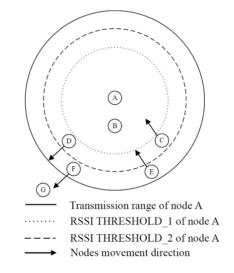
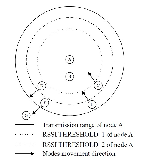
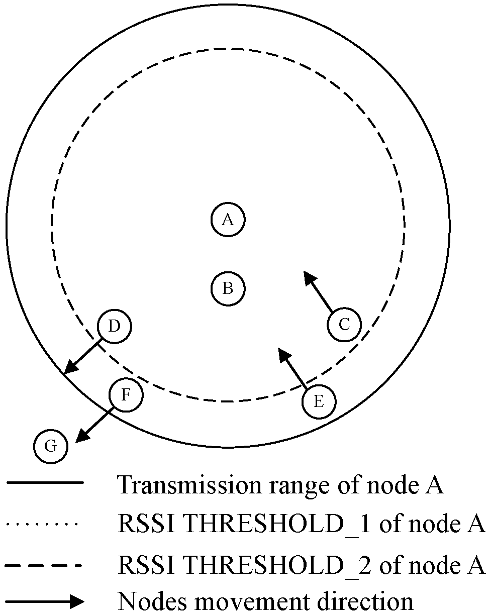
RSSI values might vary even when both nodes are not moving. Indeed, cover zones of transmitting nodes are very unstable especially in confined and complex environments. In order to take into account this phenomenon, we use two RSSI thresholds that we call $THRESHOLD\_1$ and $THRESHOLD\_2$, where $THRESHOLD\_1>THRESHOLD\_2$ as shown in Figure 1. These two thresholds will help better estimate the link quality between two nodes as follows. When a new RSSI is smaller than or equal to $THRESHOLD\_1$, the node considers that it has a good link quality with its parent node. If new RSSI is within the interval [$THRESHOLD\_2$, $THRESHOLD\_1$], the node needs to detect movement direction first and then to consider whether to stop using the link or not. In order to reduce the influence of variable coverage zone, we add a hysteresis value on the old RSSI when comparing new RSSI to old RSSI values. When the new RSSI is smaller than $THRESHOLD\_2$, only new RSSI and old RSSI will be used to estimate direction without using hysteresis. If the node is getting closer to its parent, we consider that this parent node can still be used as a next-hop. Otherwise, the parent node should be replaced.

Figure 1. The position of node B is within $THRESHOLD\_1$ of node A. Node C and node D are between $THRESHOLD\_1$ and $THRESHOLD\_2$ of node A. Node E and node F are between $THRESHOLD\_2$ and the transmission range of node A. Node G is out of the transmission range of node A, but is the neighbour of node D and node F. RSSI: received signal strength indicator.

At the initial stage, each time a node receives a DIO and adds a new node into its parents set, a timer is set for this parent. We call this timer the lifetime of a parent. A parent is kept in the parents set for the duration of its lifetime timer and can be selected as the next-hops. A parent is deleted from the parents set when the timer expires. However, before the timer expires, if a new control message is received from this parent, the timer will be reset and lifetime is renewed. According to the RRD+ mechanism, we set two sorts of lifetimes: long lifetime and short lifetime.

A long lifetime is given to the parent node in the case that the new RSSI is bigger than $THRESHOLD\_1$. In the case the new RSSI is smaller than $THRESHOLD\_1$, movement direction will be estimated first and a short lifetime is given to parent node when the movement direction is towards parent node, otherwise the rank value will be updated. When the rank value is updated, the current parent is removed from the parents set. Indeed, when the parent node is in a zone where the radio link is about to fail, a short lifetime will help avoid using this parent node for a long period in case we no longer receive its control messages.

4.2. Loop Avoidance and Rank Update

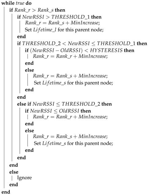
Routing loop avoidance is a challenging task in mobility scenarios. In order to avoid this, RPL uses the rank value. The rank of a node must be greater than the rank of all nodes in its potential parents set and nodes cannot forward data packets to nodes with higher or equal ranks. However, RPL does not support rank update. A current next-hop may become a descendant due to untimely update of the rank value, and loops will occur. We propose monitoring link existence and movement direction to allow nodes to update their ranks in a timely manner. The goal is to update the rank of a node when it is about to lose its link with its current parent based on the link monitoring mechanism. Algorithm 1 depicts the rank update process. $Rank\_r$ stands for the rank of the receiver of the control message and $Rank\_s$ stands for the rank of the sender of the control message. $Lifetime\_l$ stands for the long lifetime and $Lifetime\_s$ represents the short lifetime. $MinIncrease$ stands for the value of MinHopRankIncrease.

Figure 1 shows a scenario with four nodes A, B, C, D, E, F and G. A is neighbour of nodes B, C, D, E and F. D and F are neighbours of G. We use a dotted circle to represent RSSI $THRESHOLD\_1$ of node A and dashed circle to represent RSSI $THRESHOLD\_2$ of node A. Note that due to the nature of wireless signal propagation, in reality both RSSI thresholds and transmission range are most likely to look like a cloud that changes from one transmission to another. Indeed, in our simulation model we used a probabilistic propagation model to take into account coverage zone instability. B, C, D, E and F will execute Algorithm 1 whenever they receive a DIO message from A. G will execute Algorithm 1 whenever it receives a DIO message from D and F.

Algorithm 1 is explained in what follows and the scenario of Figure 1 is used as an example. When a control message is received, if the rank of receiver node ($Rank\_r$) is bigger than the rank of sender nodes ($Rank\_s$), as in the case of node B, C, D, E and F, they need to check the new RSSI value ($NewRSSI$) of the control message. If the new RSSI is bigger than $THRESHOLD\_1$, as in the case of node B, the receiver node sets a long lifetime for this parent and updates its rank $Rank\_r=Rank\_s+MinIncrease$.

Algorithm 1: Rank Update

If the new RSSI is within the interval ($THRESHOLD\_2$, $THRESHOLD\_1$), as in the case of nodes C and D, in order to avoid the influence of signal fading we set a hysteresis when estimating movement direction with the new and old RSSI. If $(NewRSSI-OldRSSI)<HYSTERESIS$, as is the case of node D, this means the receiver and the sender are getting away from each other. In this case, the receiver updates its own rank according to $Rank\_r=Rank\_r+MinIncrease$. When the rank value is updated, the children nodes of the receiver node will no longer choose it as a parent. This is the case of node G, in it that will no longer consider node D as a parent node once node D has updated its rank. Indeed, this will help avoid using a node that might lose its current link with its parent. In case receiver node moves back towards sender node, it will receive a new DIO message from the sender node and will update its rank according to the algorithm.

Otherwise, in the case $(NewRSSI-OldRSSI)\ge HYSTERESIS$, the receiver node gives a short lifetime for the sender node and updates its own rank according to $Rank\_r=Rank\_s+MinIncrease$. By this way the receiver node is only one level below the sender node. This is the case of node C. The receiver node set the parent with a short lifetime in order to avoid keeping the sender node as a parent in case the receiver node moves away from the sender node.

If the new RSSI is smaller than or equal to $THRESHOLD\_2$, as in the case of node E and F, the receiver checks the difference between the new RSSI and the old RSSI to estimate movement direction without using hysteresis. In this case the receiver node is at the edge of transmission range of the sender, thus, updating information fast is imperative, therefore the receiver ignores the hysteresis test. In this situation, if the new RSSI value is bigger than the old one, as in the case of node E, this means that the receiver is at the edge of transmission range but is moving forwards node A. In this case , node E gives a short lifetime for node A and updates its own rank according to $Rank\_r=Rank\_s+MinIncrease$. Otherwise, if the new RSSI value is smaller than the old one, as in the case of node F, this means that receiver node is getting away from the sender. In this case, node F increments its own rank by $Rank\_r=Rank\_r+MinIncrease$.

Finally, in case $Ran{k}_r$ is smaller than $Ran{k}_s$ we ignore the control messages.

4.3. Ripple Control Message Management

The trickle algorithm is used by RPL in order to reduce overhead in static networks. The trickle algorithm starts with a short interval between two DIOs in order to construct the network fast. Each time, the interval will be increased until it reaches $I_{max}$. However, when the interval increases, the trickle algorithm cannot cope with information update in a timely manner, which is important in mobility. Therefore, we propose a new DIO interval management called ripple control message management, which copes with topology changes and reduces overhead. This algorithm dynamically modifies the sending interval of DIOs according to rank updates as described in what follows.

DIO messages are broadcast by the sink node and propagated by other nodes until they reach leaf nodes. The main function of DIO messages is to help children nodes find parent nodes. If we consider the rank as a virtual range, based on the sink, the rank in the network will be like ripples in the water and the sink is the center of the ripples. We think a DIO message that comes from a lower rank is more important than a DIO message that comes from a higher rank due to the fact that lower rank DIO messages will help more nodes find parent nodes. Thus, nodes that are closer to the sink should send DIO messages more frequently and the frequency of DIO messages may be reduced for nodes with higher ranks. Hence, we designed a dynamic DIO interval management according to rank updates to reduce overhead. The DIO interval calculation is shown in Equation (3).

$$DIO\_interval=Base\_interval+Rank\times Time\_unit$$

(3)

where $DIO\_interval$ dynamically changes due to the change of rank of nodes in mobility. The $Base\_interval$ is the smallest $DIO\_interval$. $Rank$ stands for the current rank value of a node. The $Time\_unit$ is the incremental step in the DIO frequency.

5. Evaluation Results

In this section we describe our simulation set-ups and we present the evaluation results by comparing RRD+ to other RPL mobility enhancements.

5.1. Simulations Parameters

Many network simulators exist, such as Network Simulator 2 and 3, OMNeT++ (Objective Modular Network Testbed in C++), Cooja, TOSSIM (Tiny OS SIMulator), etc. We chose to use the Cooja simulator (Contiki 3.0, Adam Dunkels, Sweden). It is a emulator for Contiki systems. It is compatible with real hardware and the simulation code can be used on real-life nodes. In addition, Contiki comes with standard RPL implementation on which we added all the different enhancements including RRD+. We made some modifications on the default parameters of Cooja in order to make it more realistic, especially when it comes to emulating signal propagation. There are four propagation models in Cooja [16]. One of them is Multi-path Ray-tracer Medium (MRM) which takes reflections and refractions into account to simulate real environment. In order to make it more suitable for urban and unstable environments, we included a random behaviour to its path loss calculation. Indeed, we added a Gaussian random variable in the path loss formula of MRM in order to simulate instability of the radio links. We calibrated the randomness in order to make transmission range randomly fluctuate between 30 m and 50 m independently for each transmission. The path loss formula in decibels is shown in (4).

$$Path\_loss\left(dB\right)=min(-20,-30{log}_{10}d-30{log}_{10}f-32.45+Shadow)$$

(4)

where d is the distance in kilometres between the antennas, and f is the frequency in megahertz. Shadow stands for the Gaussian random variable in the interval $[-2,2]$ with mean value of 0 and a standard deviation of 1. With this random behaviour, we fixed the hysteresis value to $-1$. This means that if the difference between the old RSSI and the new RSSI is $1dB$, we consider that it is most probably the effect of the randomness of the propagation model and not the effect of mobility (Note that the randomness of the propagation model is related to the nature of the environment and that the value of hysteresis is closely related to the randomness of the propagation model). Table 1 summarizes the rest of the simulation parameters we used.

Table 1. Simulation setup.

Item	Parameters
Network simulator	Cooja under contiki OS (3.0)
Radio propagation model	MRM with random behaviour
Medium access control	CSMA/CA (Carrier-Sense Multiple Access with Collision Avoidance)
Simulation time	5 min
Emulated platform	Z1 starter platform
Sensor node deployment	Random deployment
Data size	30 Bytes
Transmission rate	1 pkt/s
Transmission power	−20 dBm
Transmission range	[30 m, 50 m]
Number of nodes	20, 40, 60
Area of deployment	200 m × 200 m
Frequency range	2.4 GHz
Reception threshold	−95 dBm
RRD+ RSSI $THRESHOLD\_2$	−92 dBm
RRD+ RSSI $THRESHOLD\_1$	−89 dBm
RRD+ RSSI $HYSTERESIS$	−1 dB
Long lifetime timer	30 s
Short lifetime timer	15 s

5.2. Mobility Model

We used a random waypoint model as a mobility model. At the beginning, all nodes are randomly deployed in a 200 m × 200 m area. We make sure that at the start of the simulation there are no isolated nodes. The sink is always located at the centre of the area for the duration of the simulation. When the simulation starts, each node makes a random choice to select a location within the area as a destination. Then, it moves towards this destination. The velocity is randomly chosen from 1 to 3 m/s every 5 s. We introduce rest time for each node. Whenever a node reaches its destination position, it will rest in new location for 5 s and then select a new destination for the next movement. All nodes, except the sink, repeat these steps until the simulation stops. Table 2 summarizes mobility model parameters. In addition, we considered different mobility scenarios where the ratio of mobile nodes to fixed nodes in the network varies from 100 to 25%; we call this degree of mobility. The rationale behind using random mobility scenarios is to put protocols under pessimistic mobility scenarios where the trajectory of nodes cannot be predicted. Thus, performance evaluation would show worst case scenario results.

Table 2. Mobility model parameters.

Item	Parameters
Mobility model	Random waypoint model
Minimum speed	1 m/s
Maximum speed	3 m/s
Speed changing interval	5 s
New location rest time	5 s

5.3. Simulation Results

In order to assess the efficiency of RRD+ in dealing with mobility we compared it to other existing methods studied in the related work section. These protocols are the original RPL (OR-RPL), Co-RPL [10], ME-RPL [12], and the reverse trickle timer algorithm (RT-RPL) [11]. We used four performance metrics to evaluate the efficiency of these protocols: (1) packet delivery ratio; (2) number of dropped packets; (3) average end-to-end delay; and (4) number of control packets. For each network size, we generated 10 different random mobility scenarios. Each performance metric is averaged over 10 iterations for each network size.

5.3.1. Packet Delivery Ratio

Figure 2 shows packet delivery ratio of different RPL variants based on different degrees of mobility. RRD+ outperforms other RPL and its enhancement protocols when the degree of mobility is above 25%. When the ratio of static nodes reaches 75%, RRD+ no longer has an advantage and is even outperformed by MR-RPL and RT-RPL in 60-node scenarios as shown in Figure 2d. This is mainly due to the fact that MR-RPL and RT-RPL have a mechanism to broadcast mobile nodes to other nodes in order to avoid being selected as next-hop nodes. Compared with mobile nodes, static nodes can offer more stable transmission paths. Therefore, MR-RPL and RT-RPL perform better when there are enough static nodes in the network to offer routes for the sink. On the other hand, MR-RPL and RT-RPL perform worse when there are not enough static nodes to chose from. Results also show that CO-RPL has limited contribution in mobility. This is mainly due to the fact that CO-RPL does not offer a method to update the C_ID value, which we already discussed in Section 3.

Figure 2. Packet delivery ratio. (a) Packet delivery ratio (all nodes are mobile); (b) Packet delivery ratio (75% of nodes are mobile); (c) Packet delivery ratio (50% of nodes are mobile); (d) Packet delivery ratio (25% of nodes are mobile). OR-RPL: ORiginal RPL; CO-RPL: COrona RPL; ME-RPL: Mobility-Enhanced RPL; RT-RPL: Reverse Trickle timer algorithm.

5.3.2. Number of Dropped Packets

According to the IEEE 802.15.4 MAC (Medium Access Control) layer, nodes keep retransmitting frames until the number of retransmission attempts reaches a fixed maximum value after which the frame is dropped. The number of maximum retransmissions is three according to the standard. The number of dropped packets is the number of packets that are dropped after exceeding the maximum number of retransmission attempts. This evaluation metric shows how efficient the routing protocol is in finding a new parent when the link with the current parent is lost.

Figure 3 shows the number of dropped packets of different RPL variants based on different degrees of mobility. Results show that RRD+ outperforms all other RPL variants in all scenarios. This is mainly due to the fact that RRD+ helps RPL to adapt quickly to mobility and efficient rank updating can pro-actively help nodes avoiding selecting a next-hop with a bad link quality. Therefore, RRD+ reduces retransmission attempts and the number of dropped packets is reduced as well. CO-RPL does not have proactive features, thus it suffers from a high number of dropped packets. With the increasing of the number of static nodes, ME-RPL and RT-RPL begin to show their performance for the reason discussed previously in packet delivery ratio results.

Figure 3. Number of dropped packets. (a) Number of dropped packets (all nodes are mobile); (b) Number of dropped packets (75% of nodes are mobile); (c) Number of dropped packets (50% of nodes are mobile); (d) Number of dropped packets (25% of nodes are mobile).

5.3.3. Average End-To-End Delay

Figure 4 shows the average end-to-end delay of different RPL variants based on different degrees of mobility. The delay is computed on the delivered packets, lost packets do not appear in these results. The average end-to-end delay is computed according to the following equations.

$$TotalDelay=\sum _{i=1}^n\left(RecvTime\right(i)-SentTime(i\left)\right)$$

(5)

$$AverageendtoendDelay=TotalDelay/n$$

(6)

where n refers to the number of successfully received packets.

Figure 4. Average end-to-end delay. (a) Average end-to-end delay (all nodes are mobile); (b) Average end-to-end delay (75% of nodes are mobile); (c) Average end-to-end delay (50% of nodes are mobile); (d) Average end-to-end delay (25% of nodes are mobile).

Results show that RRD+ suffers from high average end-to-end delay compared to OR-RPL, ME-RPL, and RT-RPL. The reason is that RRD+ does not have the mechanism to distinguish static nodes and mobile nodes. Therefore, compared with ME-RPL and RT-RP, RRD+ will select more mobile nodes as next-hops. Mobile nodes will indeed increase the delivery delay. CO-RPL also suffers from the same problem. The reason for CO-RPL is due to the fact that not updating C_ID would increase the number of hops during transmission, and hence, increase the delay. In addition, as we only compute delays for received packets, packets generated from lower rank nodes will have a low average end-to-end delay compared to packets generated from higher rank nodes. As with RRD+, higher rank nodes are able to successfully deliver their packets; this makes the average end-to-end delay of RRD+ higher.

5.3.4. Number of Control Packets

Figure 5 shows the number of control packets of different RPL variants based on different degrees of mobility. Results show that RRD+ outperforms CO-RPL and ME-RPL in all scenarios. This is mainly due to the fact that ripple control message management helps reduce overhead according to rank updating. Since RRD+ does not have a mechanism to distinguish static nodes and mobile nodes, there is no significant difference in overhead when the degree of mobility changes. CO-RPL periodically broadcasts DIO, therefore there is also no significant difference in overhead for different degrees of mobility. OR-RPL has the lowest overhead cost. This is mainly due to the fact that trickle algorithm, which is used in static networks, helps reduce overhead. ME-RPL suffers from a huge overhead cost when all nodes are mobile and gradually decreases the overhead when number of static nodes increases. This is mainly due to the fact that ME-RPL introduces a dynamic DIS management and ME-RPL will suffer from a huge number of DIS messages when there is more mobile nodes in the network. RT-RPL outperforms RRD+, CO-RPL and ME-RPL. The reason is that the reverse trickle algorithm is a modified trickle algorithm, which can deal with mobility and reduces overhead at the same time. However, it cannot deal with random movement, and thus compared with RRD+ it reduces overhead but does not increase the packet delivery ratio.

Figure 5. Number of control packets. (a) Number of control packets (all nodes are mobile); (b) Number of control packets (75% of nodes are mobile); (c) Number of control packets (50% of nodes are mobile); (d) Number of control packets (25% of nodes are mobile).

6. Conclusions

Dealing with mobility in WSNs and LLNs is a challenging task for which a compromise should be found between efficiency and complexity. One of the most dominant routing protocols designed for LLNs, RPL, was an original designed without special support for mobility. This is a major drawback that prevents many applications from using it. In this paper, we proposed a mobility enhancement mechanism called RRD+, designed for convergecast scenarios. RRD+ can easily be applied to the RPL routing protocol. RRD+ monitors RSSI values and updates rank values accordingly in order to avoid loops, and it also dynamically manages the interval of control messages. RRD+ monitors the direction of moving nodes based on the variation of RSSI values. When a node detects that one of its potential next-hops in the parents set is moving away, it will anticipate a link failure and try to use another node from the parents set. This helps nodes update their next-hop choice in a timely manner in mobile scenarios.

We compared RRD+ to other existing mobility enhancements for RPL and standard RPL. Simulation results show that the RRD+ mechanism enhances RPL on many levels: successfully delivered packets, packet loss, number of dropped packets, end-to-end delay, and overhead. However, results also show that RRD+ is suited for networks where more than 25% of nodes are mobile nodes. When there are fewer mobile nodes in the network, RRD+ has a limited contribution to network performance.

In our future work, we plan to add a mechanism for RRD+ to distinguish static nodes from mobile nodes in order to improve the performance of RRD+ for different degrees of mobility. Moreover, energy consumption is another critical problem we need to investigate in the future. Right now we do not use sleep mode, since topology information updating relies on information broadcasting and collection in a timely manner and a sleep mode would delay this process. RPL is energy-efficient by design; compared to other mobility supports, RRD+ has lower overhead, and thus consumes less energy. Based on this, we plan to integrate a dynamic duty cycle in RRD+ according to different degrees of mobility in order to reduce energy consumption. In the long run, it is also interesting to improve RRD+ to support mobility in data dissemination scenarios.

References

1. Tüysüz Erman, A. Multi-Sink Mobile Wireless Sensor Networks: Dissemination Protocols, Design and Evaluation; University of Twente: Enschede, The Netherlands, 2011. [Google Scholar]
2. Rawat, P.; Singh, K.D.; Chaouchi, H.; Bonnin, J.M. Wireless sensor networks: A survey on recent developments and potential synergies. J. Supercomput. 2014, 68, 1–48. [Google Scholar] [CrossRef]
3. Aminian, M.; Naji, H.R. A hospital healthcare monitoring system using wireless sensor networks. J. Health Med. Inform. 2013, 4, 121. [Google Scholar] [CrossRef]
4. Winter, T. RPL: IPv6 Routing Protocol for Low-Power and Lossy Networks; Internet Engineering Task Force (IETF): Fremont, CA, USA, 2012. [Google Scholar]
5. Levis, P.; Clausen, T.H. The Trickle Algorithm; Internet Engineering Task Force (IETF): Fremont, CA, USA, 2011. [Google Scholar]
6. Sneha, K.; Prasad, B.G. An efficient hand-off optimization based RPL routing protocol for optimal route selection in mobility enabled LLNs. In Proceedings of the 2016 International Conference on Global Trends in Signal Processing, Information Computing and Communication (ICGTSPICC), Jalgaon, India, 22–24 December 2016; pp. 130–137. [Google Scholar]
7. Gara, F.; Saad, L.B.; Hamida, E.B.; Tourancheau, B.; Ayed, R.B. An adaptive timer for RPL to handle mobility in wireless sensor networks. In Proceedings of the 2016 International Wireless Communications and Mobile Computing Conference (IWCMC), Paphos, Cyprus, 5–9 September 2016; pp. 678–683. [Google Scholar]
8. Somaa, F.; El Korbi, I.; Adjih, C.; Saidane, L.A. A modified RPL for Wireless Sensor Networks with Bayesian inference mobility prediction. In Proceedings of the 2016 International Wireless Communications and Mobile Computing Conference (IWCMC), Paphos, Cyprus, 5–9 September 2016; pp. 690–695. [Google Scholar]
9. Somaa, F.; Adjih, C.; El Korbi, I.; Saidane, L.A. A Bayesian model for mobility prediction in wireless sensor networks. In Proceedings of the International Conference on Performance Evaluation and Modeling in Wired and Wireless Networks (PEMWN), Paris, France, 22–25 November 2016; pp. 1–7. [Google Scholar]
10. Gaddour, O.; Koubâa, A.; Rangarajan, R.; Cheikhrouhou, O.; Tovar, E.; Abid, M. Co-RPL: RPL routing for mobile low power wireless sensor networks using Corona mechanism. In Proceedings of the 2014 9th IEEE International Symposium on Industrial Embedded Systems (SIES), Pisa, Italy, 18–20 June 2014; pp. 200–209. [Google Scholar]
11. Cobarzan, C.; Montavont, J.; Noel, T. Analysis and performance evaluation of RPL under mobility. In Proceedings of the 2014 IEEE Symposium on Computers and Communication (ISCC), Funchal, Portugal, 23–26 June 2014; pp. 1–6. [Google Scholar]
12. El Korbi, I.; Brahim, M.B.; Adjih, C.; Saidane, L.A. Mobility enhanced RPL for wireless sensor networks. In Proceedings of the 2012 Third International Conference on the Network of the Future (NOF), Gammarth, Tunisia, 21–23 November 2012; pp. 1–8. [Google Scholar]
13. Wang, J.; Chalhoub, G.; Tall, H.; Misson, M. Routing Protocol Enhancement for Mobility Support in Wireless Sensor Networks. In Proceedings of the International Conference on Ad-Hoc Networks and Wireless, Messina, Italy, 20–22 September 2017; Springer: Cham, Switzerland, 2017; pp. 262–275. [Google Scholar]
14. Wang, J.; Chalhoub, G.; Misson, M. Mobility support enhancement for RPL. In Proceedings of the International Conference on Performance Evaluation and Modeling in Wired and Wireless Networks, Paris, France, 28–30 November 2017. [Google Scholar]
15. Misra, I.S. Wireless Communications and Networks: 3G and Beyond; McGraw Hill Education (India) Pvt Ltd.: Bengaluru, India, 2013. [Google Scholar]
16. Stehlık, M. Comparison of Simulators for Wireless Sensor Networks. Master’s Thesis, Faculty of Informatics, Masaryk University, Brno, Czech Republic, 2011. [Google Scholar]
Article Metrics
Citations
Article Access Statistics
Multiple requests from the same IP address are counted as one view.