Abstract
Meteorological technology has evolved rapidly in recent years to provide enormous, accurate and personalized advantages in the public service. Large volumes of observational data are generated gradually by technologies such as geographical remote sensing, meteorological radar satellite, etc. that makes data analysis in weather forecasting more precise but also poses a threat to the traditional method of data storage. In this paper, we present MHBase, (Meteorological data based on HBase (Hadoop Database), a distributed real-time query scheme for meteorological data based on HBase. The calibrated data obtained from terminal devices will be partitioned into HBase and persisted to HDFS (the Hadoop Distributed File System). We propose two algorithms (the Indexed Store and the Indexed Retrieve Algorithms) to implement a secondary index using HBase Coprocessors, which allow MHbase to provide high performance data querying on columns other than rowkey. Experimental results show that the performance of MHBase can satisfy the basic demands of meteorological business services.
1. Introduction
With the evolution of Internet technology, the amount of data globally is beyond appraisal. In 2010, the global online and offline data size peaked at 1.2 Zettabytes (1 Zettabytes = 1024 EB = 1024*1024 PB) and reached to four Zettabytes in 2013 [1]. According to the prediction of the International Data Corporation (IDC), the total amount of data is expected to reach eight Zettabytes by the end of this year [2] and more than 35 Zettabytes of data will be generated by the end of this decade [3]. Data collected from meteorological fields amount to hundreds of terabytes every year. Collected data include weather information recorded at 10-minute intervals from more than 40,000 stations across the country. These collected data represent about 30% of the total meteorological data [4]. Weather satellite remote sensors and Doppler radar produce data that are calculated in terabytes daily and play an important role in real-time weather forecasting. Conventional architecture, based on IOE (IBM, Oracle and EMC), has a centralized dedicated architecture and needs expensive high-end equipment when dealing with such enormous data.
Open source cloud platforms, represented by Apache Hadoop, use horizontal scaling distributed architecture to make Big Data storage economical. The Hadoop Distributed File System (HDFS) [5] is a distributed file system designed to be operated on commodity hardware while HBase (Hadoop Database) [6] is an open source, non-relational, distributed database modeled after Google’s BigTable [7] based on HDFS. The combination of Hadoop and HBase enables reliable and expandable data storage.
It is common to use self-designed architecture to solve specific problem in specialized fields, especially in Meteorology. For example, NASA (National Aeronautics and Space Administration) uses Hadoop and Hive in RCMES (The Regional Climate Model Evaluation System) [8] to provide services and analysis based on observation data and also uses Sqoop [9] to migrate data. In another NASA project, MERRA/AS (Modern Era Retrospective-analysis for Research and Applications Analytic Services) [10], Cloudera’s CDH cluster is used to store 80 TB of data to provide data sharing and data analysis services.
In this paper, we propose a platform called MHBase (Meteorological data based on Hbase) for meteorologically structured data based on HBase in order to satisfy the business requirements of safe storage and efficiently improve the query of large meteorological data. Our other meteorological operational system uses Hadoop to store data and other components of “Hadoop ecosystem” to implement functions like Hive and Zookeeper; thus, HBase is the best choice as its features are closely combined with Hadoop. Our system is based on existing techniques such as distributed architecture and data partition strategy. Several experiments have been done to show the performance improvement for our optimized method and combined architecture. The reliability of data is ensured by a multi-copying mechanism through HDFS. In accordance with the conventional query cases, especially on HBase, we designed rowkey and to realize a secondary index.
The rest of this paper is organized as follows. Section 2 introduces some related works about our project and analyses some indexed schemes already in existence. In Section 3, we present two algorithms and detail the design and implementation of MHBase. We also evaluate performance by experimentation in Section 4. Finally, we present conclusions and future work in Section 5.
2. Related work
2.1. Distributed Architecture
The Apache Hadoop is a framework that allows for distributed processing of massive data across clusters of computers using simple programming models. Its distributed file system, named HDFS, is the open source implementation of GFS (Google File System) [11]. HDFS follows a master–slave structure, in which multiple datanodes are under the control of one “namenode”. A namenode is mainly responsible for managing metadata about where the files are stored and for what purpose as well as also preserving the mappings between files and the corresponding data blocks in memory. “Datanodes” are used to store the actual data and report block lists back to the namenode termly. Therefore, Hadoop is highly fault-tolerant and is designed to be deployed on low-cost hardware. It also provides high throughput access to application data and is extremely suitable for applications that have large data sets.
HBase is an open-source, distributed, non-relational database [12] on top of HDFS. Data are stored in HBase by (key,value)pairs. The key represents the row identifier and the value contains the row attributes. Data in HBase are modeled as a multidimensional map in which values are located by four required parameters, tablename, rowkey, family, and timestamp, and one optional parameter, qualifier. The key-value pair could be expressed as:
These kinds of data are ultimately stored in HDFS to shield the heterogeneity of the underlying system to make the cluster more reliable and the consistency of data is ensured by Zookeeper [13], a centralized service for maintaining configuration information, naming, providing distributed synchronization and group services. Figure 1 demonstrates the relationship between Hadoop and HBase.
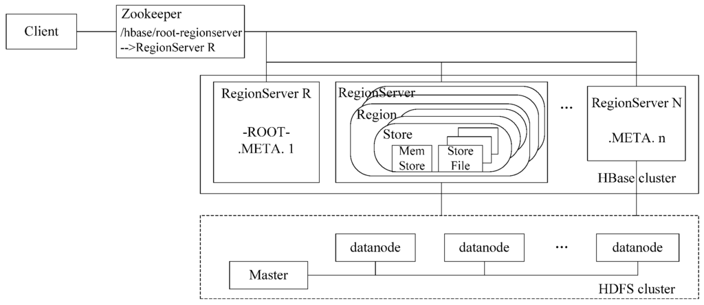
Figure 1.
The relationship between Hadoop and HBase.
There is a root table named “-ROOT-“ and a catalog table named “.META.” in HBase. -ROOT- keeps track of where the .META. table is, while the .META. table keeps a list of all RegionServers in the HBase cluster. To locate entries in three times, -ROOT- will never be divided into two. All these HBase tables are persisted into HDFS. HBase ensures load balancing via both horizontal and vertical types of data partitioning and, based on that, takes advantage of -ROOT- and .META. to locate specific entries.
2.1.1. Horizontal Partitioning
As shown in Figure 2, the table is divided into HRegions (region for short, the smallest unit of distributed storage in HBase) that are stored in different HRegionservers (also called Regionserver (RS)). Rowkey is used to address all columns in one single row and it is sorted on the basis of Log-Structured Merge Tree (LSM-Tree) [14] to speed up searching. A region will become larger with an increment in the volume of data and it will be split into two equal daughter regions when a particular threshold is reached. One RegionServer is composed of several regions but one region cannot be placed on multiple RegionServers. That is to say, a read and a write of one data entry will always be on the same RegionServer.
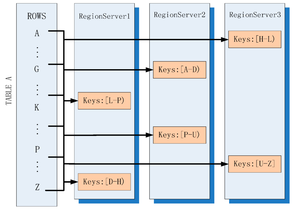
Figure 2.
Horizontal partitioning in HBase.
2.1.2. Vertical Partitioning
Each HRegion is split into individual Stores where data persist under the same family (see Figure 3) and each Store contains a MemStore and multiple StoreFiles. Data are first written onto the former and then flushed out of the latter when the predefined threshold is reached.

Figure 3.
Vertical partitioning in HBase.
From a logical viewpoint of the table, data are split horizontally across regions and then divided vertically into multiple Stores according to the families.
2.2. Meteorological Data Storage
With huge amounts of data being generated periodically in meteorological fields, the conventional IBM, Oracle and EMC architectures can no longer cope; hence, cloud computing becomes the best way to store data. Aji in Emory University presented Hadoop-GIS [15], which is a scalable and high performance spatial data warehousing system for running large-scale spatial queries on Hadoop. Hadoop-GIS supports multiple types of spatial queries on MapReduce through a spatial query engine called RESQUE that utilizes both global and customizable local spatial indexing to achieve efficient query processing. Xie and Xiong [16] achieved a linear quad-tree retrieval structure in the HBase. It uses MapReduce to insert data and create an index and also uses MapReduce to retrieve the index structure. Chuanrong Zhang from the University of Connecticut also introduced a parallel approach of MapReduce [17] for improving the query performance of geospatial ontology for disaster response. The approach focuses on parallelizing the spatial join computations of GeoSPARQL queries. All these existing systems work well in batch computations but the time for MapReduce is too long to satisfy the demands of real-time systems. Although efforts are being made to improve the real-time capability of meteorologically distributed systems, the most efficient and effective method is yet to be developed.
2.3. Optimizing
As HBase only offers the rowkey-based index [18], it can quickly look up specific records by rowkey because of the rowkey dictionary sequence. The only way to query other columns is to use a filter to perform a full-table scan, which has the effect of degrading performance. Like RDBMS, it is impossible to retrieve data using only a primary key for the meteorological application. The index scheme for HBase has always been a hot topic in open source communities. IHBase [19] is a region-level index structure that uses Bitmap [20] to organize indexes and is suitable for read-only scenarios. Furthermore, IHBase stores indexes in memory; therefore, indexes must be rebuilt every time a RegionServer crashes or restarts and this rebuild operation requires much time to complete.
Some giant companies provide their own enterprise solutions for HBase optimizing. For example, Cloudera [21] integrates Solr with HBase to present a much more flexible query and index model of HBase datasets. However, this system is complicated to deploy and it will throw exceptions unless the servers are properly tuned. The Intel® Distribution for Apache Hadoop* Software [22] includes almost all of the Hadoop ecosystems from basic project HBase to data mining project Mahout. This release has enhanced the secondary index of HBase, but it must be deployed on a node that has more than two quad-core CPUs, 16 GB RAM and does not have RAID disks.
Huawei’s recent contribution [23], which uses coprocessors to implement secondary index, is recognized as the best solution and this has attracted the attention of the open source community. Ge proposes CinHBa [24], whose index model is similar to Huawei’s contribution to provide a high-performance query capable of generating non-rowkey columns. Lastly, Apache Phoenix [25] integrates this scheme internally after version 4.1 and also provides long-term technical support. In this paper, we use this idea as a reference to propose a real-time query scheme for meteorological applications.
3. Proposed Design
In this section, we will introduce the design of MHBase considering two aspects. First, we discuss the features of data partitioning to identify the main factors in meteorological systems so that they can be taken into consideration when designing the table. Secondly, we introduce the coprocessor-based index model in detail. The architecture of MHBase is illustrated in Figure 4. Our index model is built as an enhancement on top of HBase with a server-side component that contains two expanding instances of Observer to manage the indexes and the main idea of the model is to use an index table to store the value of all indexed columns to realize the secondary index.
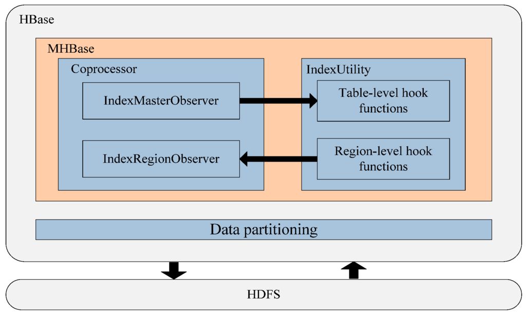
Figure 4.
Architecture of MHBase.
3.1. Data Partitioning
Hadoop ecosystem is highly extensible; therefore, HBase, unlike in a RDBMS, data distribution is done at design time [26]. HBase can be configured to use different policies for data partitioning, but for the sake of simplicity, we will use the default approach and we also optimize system performance by designing the tables’ structure.
During the horizontal partitioning phase, undesirable RegionServer hotspotting will occur at write time if the rowkey is used, which, in turn, starts with “observation time”. HBase sorts records lexicographically using the rowkey, which allows quick access to individual records, and it is always bigger, so the write operation will always be positioned in the region with the upper bound and this results particularly to RegionServer overloading. To circumvent this issue, we salted rowkey in the user table by prefixing “station number” in front of observation time. Meanwhile, rowkeys’ length should be fixed in order to improve retrieval performance.
In vertical partitioning, for a logical table in HBase, data in each family persist in a file called Store, which separates physically. Thus, we put relevant attributes into the same family so that they can be stored together on a disk at design time. For example, we put regular meteorological parameters such as rainfall, temperature, and clouds into a family named “w_info”, while the remaining unrelated information is stored in a separate family. This can improve the systems performance because non-relevant families (for current query) are not read [27]. The Store will be split into two when it is larger than a given threshold. The formula below shows how this threshold is set by default split policy.
The split threshold is defined as the minimum of: (1) a constant value of a Store’s max size; and (2) a function of the number of regions in its corresponding RegionServer (R) and the flush size of memstore.
From the beginning, the secondary element is used and data are split at a faster pace regardless of max.size. Ultimately, the split threshold will increase until it exceeds max.size. After a certain number of splits, the splitting step will remain constant from then on.
Physically, each family is separately stored in a Store; therefore, the pace of horizontal partitioning depends on the vertical design. As shown in Figure 5, with the given data, the larger the number of families, the more difficult it becomes for a Store to reach its splitting threshold. Conversely, if each family contains more attributes, it will be faster to reach the splitting threshold.
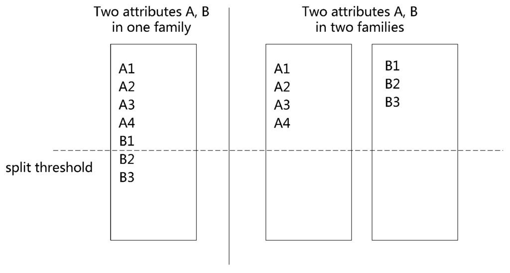
Figure 5.
Effect of vertical partitioning on region splits.
With the aim of reducing communication cost across the different RegionServers, we assumed that one server could contain both regions of the actual table (user regions for short) and their corresponding indexed tables (index regions for short) so that it can only scan the corresponding index regions while scanning user regions for one index. To achieve this goal, we used an enhanced load balancer presented by Chrajeshbabu [23] to collocate the user regions and corresponding index regions.
3.2. Index Model
This segment introduces the optimization of HBase based on coprocessors. There is an index-utility, which can be used to manage the life cycle of an index as well as an application-programming interface (API), which can also be used to serve queries based on secondary indexes. Developers can connect their applications to a cluster and execute query operations by an API, just like they would if they were using the native HBase directly.
3.2.1. Coprocessor
A Coprocessor is divided into two categories: the Observer whose function is similar to a database trigger and the Endpoint, which is similar to stored procedures in RDBMS. It can execute custom code in parallel at the region level just like a lightweight mapreduce and it also makes it possible to extend server-side functionality. Furthermore, Observer contains rich hooked functions and, for this reason, some developers have attempted to realize the index in JIRA [28,29] reports. In this paper, we add IndexMasterObserver and IndexRegionObserver, which are two expanding instances of an Observer to manage the indexes.
IndexMasterObserver is used to manage a table-level operation by a master, such as create and delete an index table automatically, while IndexRegionObserver is used to perform specific data manipulations in region-level. Table 1 shows the main functions in IndexRegionObserver.

Table 1.
The main functions in IndexRegionObserver.
When a user region is split and placed into another RegionServer, the original startkey of the upper region remains but another one should be changed and additional work has to be done by the coprocessor. These rewrite operations are triggered when regions are being compacted after region split.
The main steps are as follows:
- (1)
- get the original rowkey: , split rowkey: and their length of region startkey , ;
- (2)
- calculate the length: = the length of ;
- (3)
- new byte [];
- (4)
- copy the combination of region startkey and the rest of original rowkey to new array.
3.2.2. Algorithms
In this part, we propose two algorithms, the ISA (Indexed Store Algorithm) and the IRA (Indexed Retrieve Algorithm) to overcome problems caused by native HBase features that can only perform a full table scan by filters to retrieve exact rows when querying on columns other than rowkey. Although adding indexes will improve random read performance, we still need to examine and minimize the potential impact on write operation.
3.2.2.1. Indexed Store Algorithm (ISA)
The idea of the storage algorithm is to use an indexed table to store the values of all indexed columns. The indexes will be updated at the time of data insertion. For one row, a server-side coprocessor will match the input with predefined indexed columns. If found, it generates a new rowkey corresponding to the old one by prefixing the region’s address and index name and then puts it into the indexed table. In order to improve the performance, the put requests will be cached and then handled as a batch-put, even if there is only one Put. These puts will eventually be inserted into user table and index table, respectively.
The indexed store algorithm is shown as follows:
Algorithm 1. The Indexed Store Algorithm (ISA)
Input:
D: the actual input key-value entry
Output:
F: the set of all indexed entries of D
Procedure:
(1): get all columns in D as colList
(2): get total predefined indexes in index table as indexList
(3): get indexes columns list: idxcol = colList indexList
(4): for all idxcoliidxcol do
(5): generate a new rowkey for each index entry and put this rowkey into F
(6): end for
(7): put actual input key-value into F
(8): return F
3.2.2.2. Indexed Retrieve Algorithm (IRA)
The retrieve algorithm is roughly divided into two steps. In the first step, we set a flag depending on whether selected conditions D contain unindexed columns. In the second step, we take a random seek via indexed table for indexed columns and use filters to filter rows for unindexed columns to get result sets and then fetch the result sets according to the flag and logical relationship OP (‘AND’ / ‘OR’). Finally, the coprocessors scan the sets and return the actual results to the client. Note that it will take a full table scan if selected predicate OP is ‘OR’ and query conditions have unindexed columns. This is beyond the scope of this paper because it does not take advantage of indexes; however, the solution under this circumstance is given in our algorithm.
The indexed retrieve algorithm is shown as follows.
Algorithm 2. The Indexed Retrieve Algorithm (IRA)
T: all entries that meet any one of the search conditions
L: intermediate results according to the T and OP
Input:
D: the query conditions
OP: the logical relationship which means it matches all conditions or one condition
Output:
F: the key-value entries set
Procedure:
(1): set flag = False
(2): get all columns in D as colList
(3): get total predefined indexes in index table as indexList
(4): get indexes columns list: idxcol = colList indexList
(5): if idxcol.size < colList.size then
(6): set flag = True
(7): end if
(8): for each idxcoli idxcol do
(9): determine the index column of idxcoli
(10): generate a new rowkey of idxcoli
(11): set startkey and stopkey of scanner on the basis of changed rowkey
(12): get results by changed rowkey and add them into Ti
(13): end for
(14): if OP = Equal_All then
(15):
(16): if flag = True then
(17): filter L by using unindexed columns in D and refresh L
(18): end if
(19): else if OP = Equal_One then
(20):
(21): if flag = True then
scan table to fiter data on unindexed columns in D and append results to L
(22): end if
(23): end if
(24): F = use each key in L as rowkey to get exact rows
(25): return F
The columns in query condition must first be checked on the server side. For example, server gets idxcol, which is intersected with colList (total qualifiers in query condition D) and indexList (predefined indexes in index table) in the first step. If the size of idxcol is smaller than colList, it suggests that query condition contains unindexed columns. Thus, we set the flag True. After that, we use the IndexRegionObserver, an enhanced subclass instance of the coprocessor method above to traverse the idxcol to decide which index these columns belong to. In each iteration, there is a match between index and column and it will return a new key that contains an index name and the field value. Next, IndexRegionObserver creates a scanner prefixed with the key that determines the start and stop locations on each region and equally retrieves the region.
4. Experiments and Analyses
In this section, we conduct a comprehensive assessment through the experiments on the MHBase. Our experiments are conducted on a four-machine cluster, in which each machine uses default configurations in order to reduce influences on performance caused by various configuration settings. We deploy MHBase based on Hadoop-1.0.4 with an embedded ZooKeeper, the cluster-management component. One machine contains a master node and three Regionservers (the other three machines), all of which are connected together via a gigabit Ethernet. Specific machine parameters and configuration settings are listed in Table 2.

Table 2.
Configurations of the cluster
We take weather data from 1949 to 2014 and chose the most commonly used seventeen attributes from 120 fields included in observed site information. They are classified into two categories: identity fields and observed fields. In our experiments, we design rowkey with the combination of “station number”, “observation time (including year, month, day and hour)” and “data type”. The length of each column in rowkey should be fixed to identify the meaning of each digit conveniently. Other identity fields such as “country number”, “longitude”, “latitude” and “station style” are stored in one column family. We use another column family to store observed fields. The table structure is described in Table 3. Indexes have been built on top of 14 attributes among 17 columns. Our goal is to transfer a business platform from RDBMS to a cloud environment in order to improve price/performance ratio; therefore, we compare the different dataset sizes (records) between MHBase and MySQL.

Table 3.
HBase table structure of meteorological data.
We have selected ten common queries, including querying by “observation time”, “country number”, etc. and the test performance for each case is the average of five times. Figure 6 shows the average time consumed by MySQL and MHBase. We discontinue testing MySQL without indexes because the query time had already reached more than seven seconds in five million rows.
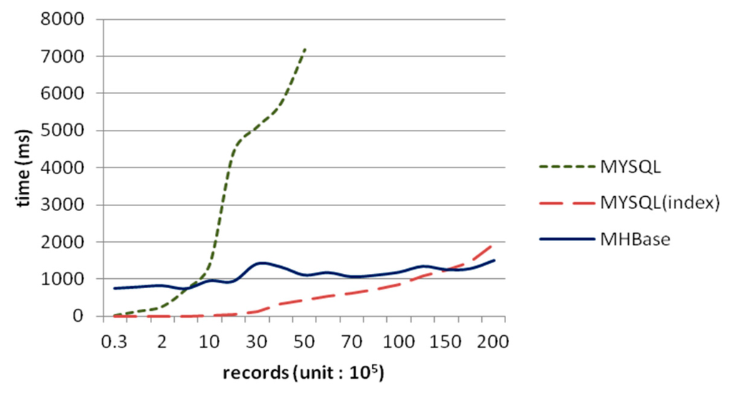
Figure 6.
Query time in weather dataset.
Just as Figure 7 shows, the execution time of importing dataset into HBase and MHbase is stable. Although the performance of MySQL with indexes is excellent in small datasets, it began to decline with the increasing data scales. In addition, the speed of data import goes down significantly. Nevertheless, MHBase retrieves records via coprocessors in region-level, and the rowkey of the table in HBase is in lexicographical (alphabetical) order, so time consumption can be considered as a linear trend of growth. Note that the performance of MHBase is also better than MySQL with indexes from 18 million rows. It implies that MHBase will be more efficient in dealing with large-scale data.
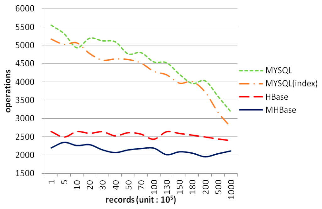
Figure 7.
The time of data import.
We already know that HBase would trade off read efficiency on fields other than the primary key. Thus, the only way to search columns without rowkey is to take up a full table scan by a filter. As a consequence, we also make a comparison between MHBase and HBase with filters within 150,000 rows and the result in Figure 8 shows that filters cost more time because filters scan a full HBase table, while the time of MHBase can be thought as constant.
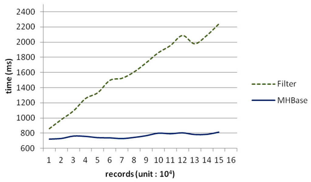
Figure 8.
Performance in different data size.
An optimized query-by-filter method is more efficient at creating a scanner with a prefix-match first, and then filter data on other columns in the range of a start key and a stop key. For example, if we want all records generated from a station with number “210044001”, we can set “210044001” as start key and “210044001” + “/0xffff” as the stop key and then use filters to retrieve columns other than rowkey because our rowkey starts with the station number and observed time. However, this scenario is impractical and lacks credibility, so we just use this special query case to illustrate the performance of MHBase. Figure 9 shows the time of same query case between MHBase and HBase (query by prefix).
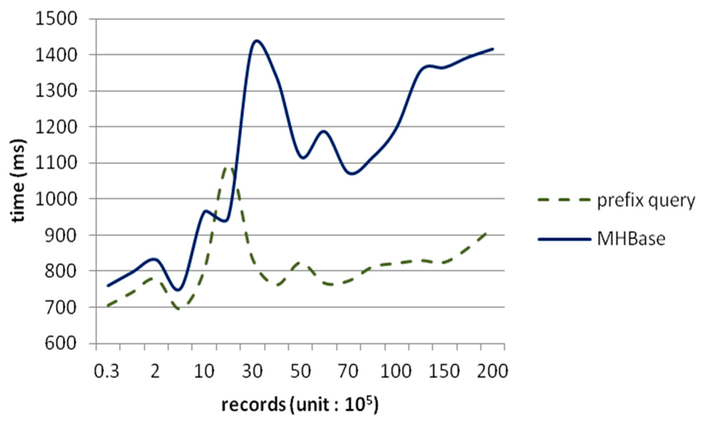
Figure 9.
Time of indices query and prefix query.
As shown in Figure 10, prefix matched queries can locate the range of target region directly and accurately, and afterwards filters work in the specific range. But MHBase use coprocessors to get records in a parallel approach; that is, the essence of an indexed query is one prefix-match and one rowkey-get operation, so it will be slower than retrieving directly by rowkey. The reason for the raised interval between two million and three million in the picture is that the region splitting causes I/O load to rise. The query’s response time for both methods are close to each other using millions of data but the diversity of retrieval by MHBase is increased.
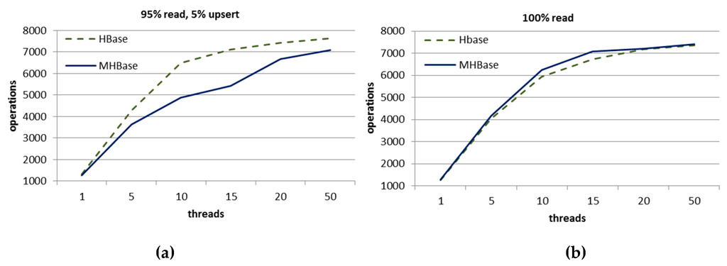
Figure 10.
Performance in different circumstance: (a) 100% read operations; and (b) 95% read and 5% upsert operations.
We also use YCSB (Yahoo! Cloud Serving Benchmark) [30] to conduct stress tests on both MHBase and HBase. We test the performance with different pressure. As shown in the Figure 10a, it is observed that the throughput of MHBase will reduce and is lower than native HBase when inserting data using ten threads concurrently and its write operation is not so excellent because MHBase needs to write to the index table synchronously. In Figure 10b, there is almost no difference in 100% read circumstance. Generally, both throughputs are improved with the increase of pressure (threads).
As our experimental results show, with the benefit of indexes, MHBase can greatly improve the querying speed, even if there is a slight performance penalty in write operation, and provide multiplicity and high performance of data accesses on non-primary keys. That is to say, MHBase achieves a balance in read and write performance because data import in our meteorological system is offline. On the other hand, we use HDD and other PC equipment as base installation to gain better performance instead of expensive commercial equipment such as SSD or RAID, so the price/performance ratio is improved. In a nutshell, MHBase is able to manage and maintain indexes effectively to make query more efficient and also meet the requirements of meteorological applications.
5. Conclusions and Future Work
In this paper, we proposed MHBase, a distributed real-time query scheme for meteorological data based on HBase, which aims to satisfy the demands of a query’s performance when facing huge amounts of meteorologically structured data. We explained the different influences on different datasets with respective split strategies and also developed two algorithms (the ISA and the IRA) to implement indexing by coprocessor. Finally, our findings were verified by experimentation and the results were compared. Our design achieved a balance between read and write performance and greatly improved the performance of a query. All these findings are evidence that MHBase is of practical significance in meteorological applications when compared to RDBMS. In our future work, we will use this solution in domains other than meteorology.
Acknowledgments
This work was supported in part by National Science Foundation of China (No. 61572259), Special Public Sector Research Program of China (No. GYHY201506080) and PAPD.
Author Contributions
Tinghuai Ma and Xichao Xu conceived and designed the experiments; Xichao Xu performed the experiments; Meili Tang and Wenhai Shen analyzed the data; and Xichao Xu wrote the paper.
Conflicts of Interest
The authors declare there are no conflicts of interest regarding the publication of this paper.
Abbreviations
The following abbreviations are used in this manuscript:
| MHBase: | Meteorological data based on HBase |
| HBase: | Hadoop Database |
| IHBase: | Indexed HBase |
| HDFS: | the Hadoop Distributed File System |
| RDBMS: | Relational Database Management System |
| PAPD: | A Project Funded by the Priority Academic Program Development of Jiangsu Higher Education Institutions |
References
- Feldman, M.; Friedler, S.A.; Moeller, J.; Scheidegger, C.; Venkatasubramanian, S. Certifying and removing disparate impact. In Proceedings of the 21th ACM SIGKDD International Conference on Knowledge Discovery and Data Mining, New York, NY, USA, 10–13 August 2015; pp. 259–268.
- Gantz, J.; Reinsel, D. Extracting value from chaos. IDC iview 2011, 9–10. [Google Scholar]
- Islam, N.S.; Rahman, M.W.; Jose, J.; Rajachandrasekar, R.; Wang, H.; Subramoni, H.; Murthy, C.; Panda, D.K. High performance RDMA-based design of HDFS over InfiniBand. In Proceedings of the International Conference on High Performance Computing, Networking, Storage and Analysis, Los Alamitos, CA, USA, 10–16 November 2012; p. 35.
- Ma, T.; Lu, Y.; Shi, S.; Tian, W.; Wang, X.; Guan, D. Data resource discovery model based on hybrid architecture in data grid environment. Concurr. Comp-Pract. E. 2015, 27, 507–525. [Google Scholar] [CrossRef]
- Shvachko, K.; Kuang, H.; Radia, S.; Chansler, R. The hadoop distributed file system. In Proceedings of the 2010 IEEE 26th Symposium on Mass Storage Systems and Technologies (MSST), Incline Village, NV, USA, 3–7 May 2010; pp. 1–10.
- George, L. The region life cycle. In HBase: the definitive guide; George, L., Ed.; O’Reilly Media: Sebastopol, CA, USA, 2011; pp. 328–330. [Google Scholar]
- Li, D.; Wang, Y.; Xiong, A.; Ma, T. High Performance Computing Model for Processing Meteorological Data in Cluster System. J. Convergence Inf. Technol. 2011, 6, 92–98. [Google Scholar]
- Mattmann, C.A.; Waliser, D.; Kim, J.; Goodale, C.; Hart, A.; Ramirez, P.; Crichton, D.; Zimdars, P.; Boustani, M.; Lee, K.; et al. Cloud computing and virtualization within the regional climate model and evaluation system. Earth Sci. Inform. 2014, 7, 1–12. [Google Scholar] [CrossRef]
- Aravinth, M.S.S.; Shanmugapriyaa, M.S.; Sowmya, M.S.; Arun, M.E. An efficient HADOOP frameworks SQOOP and ambari for big data processing. IJIRST 2015, 1, 252–255. [Google Scholar]
- Rienecker, M.M.; Suarez, M.J.; Gelaro, R.; Todling, R.; Bacmeister, J.; Liu, E.; Bosilovich, M.G.; Schubert, S.D.; Takacs, L.; Kim, G.K.; et al. MERRA: NASA’s modern-era retrospective analysis for research and applications. J. Climate 2011, 24, 3624–3648. [Google Scholar] [CrossRef]
- Ghemawat, S.; Gobioff, H.; Leung, S.T. The Google file system. In Proceedings of the nineteenth ACM symposium on Operating systems principles, New York, NY, USA, 19–22 October 2003; Volume 37, pp. 29–43.
- Cattell, R. Scalable SQL and NoSQL data stores. ACM SIGMOD Record 2011, 39, 12–27. [Google Scholar] [CrossRef]
- Hunt, P.; Konar, M.; Junqueira, F.P.; Reed, B. ZooKeeper: Wait-free coordination for internet-scale systems. In Proceedings of the USENIX Annual Technical Conference, Boston, MA, USA, 23–25 June 2010; p. 9.
- Zhao, Y.; Ma, T.; Liu, F. Research on index technology for group-by aggregation query in XML cube. Inf. Technol. J. 2010, 9, 116–123. [Google Scholar] [CrossRef]
- Aji, A.; Wang, F.; Vo, H.; Lee, R.; Liu, Q.; Zhang, X.; Saltz, J. Hadoop GIS: A high performance spatial data warehousing system over mapreduce. In Proceedings of the VLDB Endowment, Riva del Garda, Italy, 26–30 August 2013; pp. 1009–1020.
- Xie, X.; Xiong, Z.; Zhou, G.; Cai, G. On massive spatial data cloud storage and quad-tree index based on the Hbase. WIT. Trans. Inf. Commun. Technol. 2014, 49, 691–698. [Google Scholar]
- Zhang, C.; Zhao, T.; Anselin, L.; Li, W.; Chen, K. A Map-Reduce based parallel approach for improving query performance in a geospatial semantic web for disaster response. Earth. Sci. Inform. 2014, 8, 499–509. [Google Scholar] [CrossRef]
- Fong, L.L.; Gao, Y.; Guerin, X.; Liu, Y.G.; Salo, T.; Seelam, S.R.; Tan, W.; Tata, S. Toward a scale-out data-management middleware for low-latency enterprise computing. IBM. J. Res. Dev. 2013, 57, 1–6. [Google Scholar] [CrossRef]
- IHBase. Available online: http://github.com/ykulbak/ihbase (accessed on 8 July 2010).
- Chan, C.Y.; Ioannidis, Y.E. Bitmap index design and evaluation. In Proceedings of the 1998 ACM SIGMOD international conference on Management of data, New York, NY, USA, 1–4 June 1998; pp. 355–366.
- Hbase-solr-indexer. Available online: http://archive.cloudera.com/cdh5/cdh/5/hbase-solr-1.5-cdh5.3.3.tar.gz (accessed on 9 April 2015).
- The Intel Distribution for Apache Hadoop* Software. Available online: http://www.intel.com/content/www/uk/en/big-data/big-data-intel-distribution-for-apache-hadoop.html (accessed on 29 April 2013).
- Hindex. Available online: https://github.com/Huawei-Hadoop/hindex (accessed on 30 September 2013).
- Ge, W.; Huang, Y.; Zhao, D.; Luo, S.; Yuan, C.; Zhou, W.; Tang, Y.; Zhou, J. CinHBa: A secondary index with hotscore caching policy on Key-Value data store. In Proceedings of the 10th International Conference, Guilin, China, 19–21 December 2014; pp. 602–615.
- Foundation, A.S. Apache Phoenix. Available online: http://phoenix.apache.org (accessed on 8 April 2015).
- Romero, O.; Herrero, V.; Abelló, A.; Ferrarons, J. Tuning small analytics on Big Data: Data partitioning and secondary indexes in the Hadoop ecosystem. Inform. Syst. 2015, 54, 336–356. [Google Scholar] [CrossRef]
- Özsu, M.T.; Valduriez, P. Parallel Database Systems. In Principles of Distributed Database Systems; Özsu, M.T., Valduriez, P., Eds.; Springer: New York, NY, USA, 2011; pp. 497–550. [Google Scholar]
- George, P.S. [HBASE-2426] Introduce quick scanning row-based secondary indexes. Available online: https://issues.apache.org/jira/browse/HBASE-2426 (accessed on 8 April 2011).
- Shi, X. [HBASE-5723] Simple Design of Secondary Index. Available online: https://issues.apache.org/jira/browse/HBASE-5723 (accessed on 5 April 2012).
- Cooper, B.F.; Silberstein, A.; Tam, E.; Ramakrishnan, R.; Sears, R. Benchmarking cloud serving systems with YCSB. In Proceedings of the 1st ACM symposium on Cloud computing, New York, NY, USA, 10–11 June 2010; pp. 143–154.
© 2016 by the authors; licensee MDPI, Basel, Switzerland. This article is an open access article distributed under the terms and conditions of the Creative Commons by Attribution (CC-BY) license (http://creativecommons.org/licenses/by/4.0/).