Article

Explainable Graph Neural Networks for Multi-Class Fraudulent Address Classification in Ethereum

1
Department of Information Security, Faculty of Information Technology, University of Petra (UoP), Amman 11196, Jordan
2
Department of Information Technology, King Abdullah II School for Information Technology, University of Jordan (JU), Amman 11942, Jordan
3
Artificial Intelligence Research Center (AIRC), College of Engineering and Information Technology, Ajman University, Ajman P.O. Box 346, United Arab Emirates
4
Department of Cybersecurity, College of Computing, Umm Al-Qura University, Makkah 24381, Saudi Arabia
*
Author to whom correspondence should be addressed.
Future Internet 2026, 18(9), 461; https://doi.org/10.3390/fi18090461
Submission received: 17 July 2026 / Revised: 24 August 2026 / Accepted: 25 August 2026 / Published: 28 August 2026

Abstract

Blockchain networks have become a major target for fraudulent activities, including phishing and scamming attacks, due to the irreversible and pseudonymous nature of cryptocurrency transactions. Existing Ethereum fraud detection studies commonly formulate the problem as a binary classification task, which limits their ability to distinguish among different malicious behaviors. This paper proposes an explainable Graph Neural Network-based framework for multi-class Ethereum address classification using an enhanced version of the Benchmark Labeled Transactions Ethereum (BLTE) dataset. The original binary BLTE dataset is extended into a multi-class dataset by integrating external attack-category information and labeling addresses as Normal, Phishing, or Scamming. The resulting BLTE multi-class dataset contains 73,033 Ethereum addresses, 23 behavioral node features, and 6588 directed transaction edges. Three GNN architectures, namely Graph Attention Network (GAT), Graph Convolutional Network (GCN), and GraphSAGE, are evaluated under identical experimental settings. Across ten stratified random seeds, GraphSAGE achieves the best overall performance among the implemented GNNs, with 98.84 ± 0.06 % accuracy, 80.42 ± 2.67 % macro recall, 51.08 ± 1.54 % macro F1-score, and 99.27 ± 0.03 % weighted F1-score. To improve model transparency, GNNExplainer is used to identify influential transaction subgraphs and important node features that contribute to each prediction. The results indicate that neighborhood-aware graph learning is useful for multi-class Ethereum address classification, while also showing that minority-class precision remains challenging under severe class imbalance. A feature-only multilayer perceptron is found to be a strong baseline whose macro F1-score is statistically indistinguishable from GraphSAGE after multiple-comparison correction; the improvement attributable to graph structure is therefore modest and concentrated on the small connected portion of the network, and external validation on independent datasets is still required before the framework is used in real investigations.

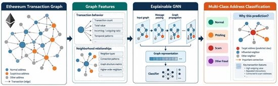
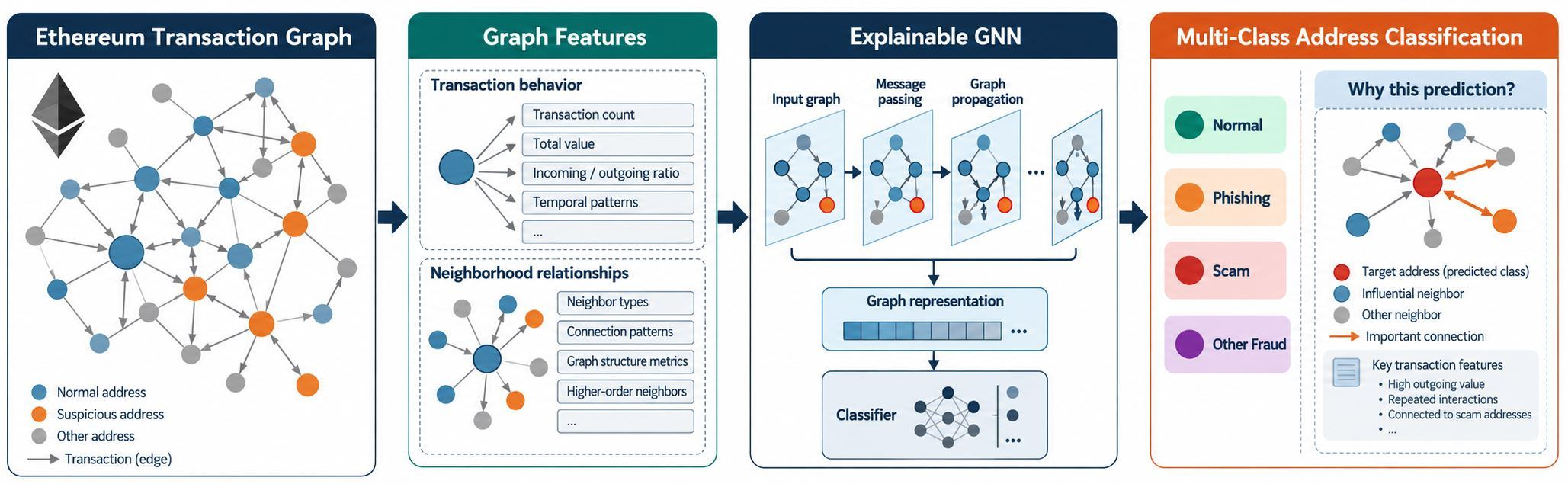
Graphical Abstract

1. Introduction

Blockchain technology has emerged as a fundamental infrastructure for decentralized digital services, cryptocurrency exchange, smart-contract execution, and decentralized finance applications. Among existing blockchain platforms, Ethereum has gained significant attention for supporting programmable smart contracts and enabling transparent peer-to-peer financial interactions. However, despite these advantages, Ethereum has also become an attractive environment for malicious activities because transactions are pseudonymous, publicly accessible, and irreversible once confirmed. Consequently, fraudulent activities such as phishing, scamming, fake investment schemes, and other abnormal transaction behaviors have become critical threats to users, service providers, and the broader blockchain ecosystem [1].
Detecting fraudulent Ethereum addresses is, therefore, an important research problem in blockchain security. Traditional fraud detection approaches commonly rely on handcrafted transaction features and conventional machine learning classifiers. Although such methods can identify some suspicious behaviors, they often treat each address or transaction as an independent record. However, Ethereum transaction data are inherently relational because addresses interact with one another through directed transaction flows. Fraudulent addresses may also exhibit distinctive topological patterns, repeated interactions, concentrated incoming transactions, abnormal temporal activity, and unusual neighborhood structures. Therefore, ignoring the graph-based relationships among Ethereum addresses may limit detection models’ ability to capture hidden fraud patterns within the transaction network.
Recent studies have increasingly explored graph-based learning for Ethereum fraud detection. For example, temporal graph attention models have been proposed to capture dynamic phishing behavior in Ethereum transaction networks [2], while hybrid graph neural models have been used to address feature extraction and class imbalance in phishing scam detection [3]. Furthermore, ego-graph augmentation strategies have been introduced to improve phishing detection by enhancing local structural representations of Ethereum accounts [4]. These studies demonstrate the effectiveness of graph learning for blockchain security. Nevertheless, most existing approaches remain focused mainly on binary detection or phishing-specific classification. As a result, they provide limited insight into different types of malicious behavior, such as distinguishing between phishing and scamming activities.
In addition, many existing Ethereum fraud detection studies formulate the problem as a binary classification problem, in which addresses are labeled only as Normal or Abnormal. Although binary classification is useful for general anomaly detection, it is insufficient for practical blockchain forensic analysis because security analysts often require more detailed information about the nature of the detected threat. For instance, a phishing address may exhibit different interaction patterns from a scamming address, and treating both categories as a single abnormal class may obscure important behavioral differences. Accordingly, a multi-class classification framework is needed to provide more fine-grained detection and support more informative blockchain security analysis.
Moreover, the severe class imbalance commonly observed in blockchain fraud datasets presents an additional challenge. In real Ethereum transaction networks, malicious addresses account for only a very small fraction of all observed addresses. Therefore, high overall accuracy may be misleading if a model mainly learns the majority normal class while failing to detect rare fraudulent classes. Recent blockchain anomaly detection studies have highlighted the importance of addressing imbalance, temporal behavior, and graph structure when modeling suspicious transaction activities [5]. Consequently, evaluation metrics such as macro precision, macro recall, macro-F1, weighted F1-score, and confusion matrices are necessary to assess model performance more comprehensively.
Another important challenge is model interpretability; Deep Learning (DL) and Graph Neural Network (GNN) models can achieve strong predictive performance, but they are often considered black-box models because their decisions are difficult to explain. However, in blockchain security applications, interpretability is essential because investigators need evidence explaining why a wallet address has been classified as suspicious. Explainable graph learning methods are therefore important for identifying influential transaction relationships, relevant neighboring nodes, and important node features that contribute to a model prediction [6,7]. Hence, an effective Ethereum fraud detection framework should not only achieve high detection performance but also provide interpretable evidence to support analyst-oriented decision making.
To address these limitations, this paper proposes an explainable Graph Neural Network-based framework for multi-class Ethereum fraud detection using an enhanced version of the Benchmark Labeled Transactions Ethereum (BLTE) dataset https://github.com/salam-ammari/Labeled-Transactions-based-Dataset-of-Ethereum-Network (accessed on 23 August 2026). First, the original binary BLTE dataset is extended into a multi-class version by integrating external attack-category information [8]. Ethereum addresses are labeled as Normal, Phishing, or Scamming. Second, the enhanced dataset is transformed into a directed Ethereum transaction graph, in which addresses are represented as nodes, transaction relationships as edges, and behavioral transaction features as node attributes. This graph formulation enables the proposed models to learn from both address-level features and transaction-neighborhood structures.
Furthermore, three representative Graph Neural Network architectures are investigated: Graph Attention Network (GAT) [9], Graph Convolutional Network (GCN) [10], and GraphSAGE [11]. These models are selected because they represent different graph learning mechanisms. GAT uses attention-based aggregation to assign different importance weights to neighboring nodes, GCN performs convolutional message passing over graph neighborhoods, and GraphSAGE learns node embeddings through neighborhood sampling and aggregation. By evaluating these models under identical experimental settings, this study provides a comparative analysis of attention-based, convolution-based, and sampling-based GNN strategies for Ethereum fraud detection.
In addition, this work integrates GNNExplainer to improve the transparency of the proposed framework. GNNExplainer is applied after model training to identify influential transaction subgraphs and important node features that contribute to each prediction [6,12]. Therefore, the proposed approach supports both automated multi-class fraud detection and explainable blockchain forensic analysis. The main contributions of this paper are summarized as follows:
  • A multi-class version of the BLTE dataset is constructed by enriching the original binary labels with attack-category information, enabling Ethereum addresses to be classified as Normal, Phishing, or Scamming.
  • The enhanced dataset is transformed into a directed Ethereum transaction graph that preserves address-level features and transaction relationships, making it suitable for GNN learning.
  • Three GNN architectures, namely GAT, GCN, and GraphSAGE, are implemented and evaluated for multi-class Ethereum fraud detection under the same experimental conditions.
  • GNNExplainer is incorporated to provide interpretable explanations by identifying the most influential transaction edges, neighboring nodes, and node features contributing to model predictions.
  • The three GNN families are compared against strong feature-only learners (MLP, Random Forest, and XGBoost) and a re-implemented published graph baseline under a repeated ten-seed protocol with paired significance testing, effect sizes, and confidence intervals, so that the contribution of graph structure is disentangled from that of the address-level behavioral features rather than assumed.
  • The explanations are evaluated quantitatively using fidelity, sparsity, and stability, and their cross-seed robustness is reported, moving the interpretability analysis beyond single-instance illustrations that are common in prior Ethereum fraud detection work.
The remainder of this paper is organized as follows. Section 2 reviews related work on Ethereum fraud detection, blockchain intrusion detection, graph-based learning, and XAI. Section 3 presents the proposed methodology, including the construction of the multi-class BLTE dataset, preprocessing, graph construction, GNN-based node classification, GNNExplainer-based explainability, and evaluation metrics. Section 4 provides the experimental setup, including the robustness-extension protocol for multi-seed evaluation, baselines, significance testing, and label-independent edge reconstruction. Section 5 reports and discusses the experimental results for GAT, GCN, and GraphSAGE. Section 6 provides a comparative evaluation of the investigated GNN models in terms of classification performance, training behavior, and interpretability, and includes an ablation study and a quantitative evaluation of the explanations. Section 7 discusses the threats to validity and limitations of the study. Finally, Section 8 concludes the paper.

2. Related Work

Research on detecting fraudulent activity in the Ethereum network has evolved from conventional feature-engineering pipelines toward graph-based DL, accompanied by a growing interest in model explainability. This section reviews the most relevant directions and positions the present work with respect to them.

2.1. Feature-Based and Conventional Learning Approaches

Early approaches to Ethereum fraud detection treat each address or transaction as an independent record and rely on handcrafted statistical features combined with conventional machine learning classifiers. To support such studies, Al-E’mari et al. [8] introduced the BLTE dataset, which provides address-level behavioral attributes along with binary normal/abnormal labels and has since served as a basis for several detection models. Building on this dataset, Sanjalawe and Al-E’mari [13] proposed ATD-SGAN, a semi-supervised generative adversarial network that synthesizes additional abnormal transaction samples to mitigate class imbalance; the approach reports improvements in detection accuracy of between 3.78% and 11.05% over competing intrusion detection systems while substantially reducing the false alarm rate. Although these methods demonstrate that behavioral features carry useful discriminative signals, they largely ignore the relational structure of the transaction network and formulate detection as a binary problem, which limits their ability to distinguish between qualitatively different malicious behaviors.

2.2. Graph-Based Learning for Ethereum Fraud Detection

Because Ethereum transactions are inherently relational, recent work increasingly models the network as a graph and applies graph representation learning. Li et al. [14] construct lightweight transaction subgraphs around labeled phishing accounts and apply a Chebyshev Graph Convolutional Network for phishing detection, while Xiong et al. [15] build a directed multi-transaction graph and combine random-walk-based feature learning with Graph Neural Networks. Temporal dynamics have also been incorporated: Wang et al. [2] propose a temporal Graph Attention Network that captures the evolving interaction patterns of phishing accounts, and Han et al. [16] introduce a multi-layer temporal transaction anomaly detection framework that couples temporal modeling with Graph Neural Networks. To address the severe class imbalance and limited feature expressiveness common to this domain, Chen et al. [3] combine a data-augmentation strategy with a hybrid Graph Neural Network, and Chen et al. [17] fuse multiscale features within a graph convolutional architecture. Structural augmentation has likewise been explored, with Huang et al. [4] proposing an ego-graph augmentation scheme (PEAE-GNN) that enriches the local structure of Ethereum accounts. At the network-forensics level, Liu et al. [18] move beyond single-account detection to uncover coordinated phishing gangs from blockchain data. Collectively, these studies confirm the value of graph-based learning for blockchain security; however, the great majority remain focused on binary detection or on phishing in isolation, and therefore provide limited support for the fine-grained, multi-class characterization of malicious behavior that forensic analysts require.

2.3. Explainability in Graph Neural Networks

The opacity of Graph Neural Networks has motivated a parallel line of work on interpretability. Ying et al. [12] propose GNNExplainer, a model-agnostic, post hoc method that identifies a compact subgraph and a subset of node features that are most responsible for a given prediction by maximizing the mutual information between the prediction and the explanation. Yuan et al. [6] subsequently provide a taxonomic survey of explanation techniques for Graph Neural Networks, situating GNNExplainer within the broader landscape of instance-level and model-level approaches. Despite the clear relevance of interpretability to blockchain forensics, where investigators must justify flagging an address, explainability has rarely been integrated into Ethereum fraud detection pipelines, and comparative analyses of how different graph architectures reach their decisions remain scarce.

2.4. Research Gap

In summary, existing studies establish that graph-based learning is effective for Ethereum fraud detection and that explanation methods can render graph models more transparent, but three gaps persist. First, most detection models are binary or phishing-specific and cannot differentiate between distinct fraud categories, such as phishing and scamming. Second, the BLTE dataset, despite its rich behavioral features, has been used almost exclusively in a binary setting. Third, explainability is seldom incorporated into the detection pipeline, and the explanatory behavior of competing graph architectures is rarely compared on the same data. Table 1 summarizes representative studies along these dimensions and positions the present work with respect to them. The present work addresses the identified gaps by extending BLTE into a multi-class dataset, evaluating three representative Graph Neural Network architectures (GAT, GCN, and GraphSAGE) under identical conditions, and integrating GNNExplainer to provide architecture-level interpretability for fine-grained Ethereum fraud detection. Unlike prior graph-based Ethereum studies, which typically report a single architecture on a single split, the present study contributes a controlled, identical-setting comparison of attention-, convolution-, and sampling-based GNNs together with strong feature-only and published graph baselines, a repeated-seed significance analysis that explicitly quantifies how much of the performance is attributable to graph structure versus node features, and a quantitative evaluation of explanation quality; these elements, rather than any single new architecture, constitute the methodological contribution.

3. Proposed Method

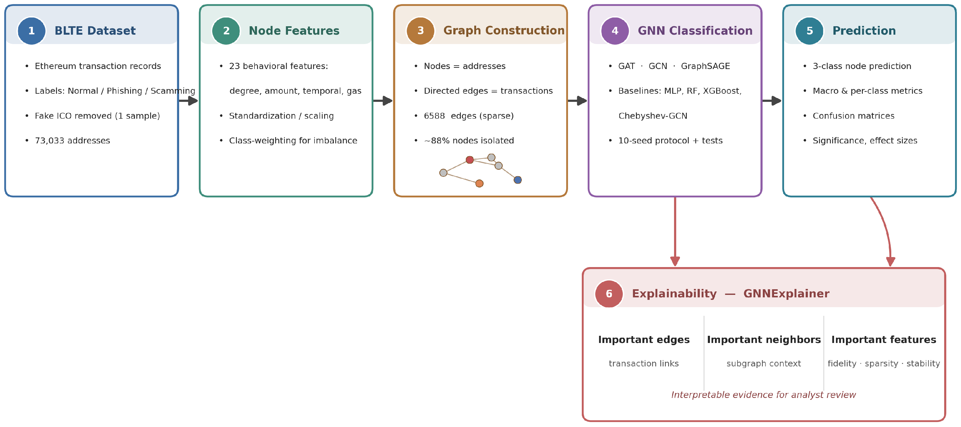
This section presents the proposed methodology for multi-class classification of fraudulent Ethereum addresses. The overall workflow is illustrated in Figure 1, which summarizes the main stages of the framework, beginning with the construction of the multi-class BLTE dataset and the extraction of behavioral node features, followed by Ethereum transaction graph construction, GNN-based node classification using GAT, GCN, and GraphSAGE, and finally the application of GNNExplainer to provide interpretable evidence for model predictions. Each stage is described in detail in the following subsections.

3.1. Multi-Class BLTE Dataset

The original BLTE dataset was developed to support abnormal transaction detection in Ethereum networks using a binary classification setting, where each Ethereum address was labeled as either Normal or Abnormal. Although this binary formulation is useful for detecting suspicious activity, it does not provide sufficient semantic information about the specific type of fraudulent behavior. Therefore, in this work, the original BLTE dataset was extended into a multi-class version, referred to as BLTE multi-class, to enable fine-grained classification of Ethereum addresses into Normal, Phishing, and Scamming categories.
The multi-class transformation was performed by integrating the original BLTE address-level dataset with an external attack-category dataset. This dataset contains Ethereum transaction relationships and attack category information associated with sender and receiver addresses. Since Ethereum addresses may appear in different formats, all addresses were first normalized by converting them to lowercase and removing leading and trailing spaces. This normalization was applied to the Address field in BLTE, as well as the from_address and to_address fields in the attack-category dataset.
The attack-category fields from_category and to_category were then processed to extract valid fraud labels. Empty, null, or invalid category values were replaced with missing values and excluded from the attack lookup table. Two label sets were created: one from sender-side attack categories and one from receiver-side attack categories. These two sets were then combined into a unified attack-address lookup table. If an Ethereum address appeared multiple times across different category records, the most frequent attack category was assigned to that address. This strategy reduces inconsistency in the labeling process and ensures that each address receives only one final attack label. After constructing the attack lookup table, it was merged with the original BLTE dataset using the normalized Ethereum address as the key. Addresses that appeared in the attack-category dataset were assigned their corresponding fraud class, while addresses that did not appear in the external attack repository were labeled as Normal. It is important to state the assumption underlying this rule explicitly. The external attack repository is a positive-only source: it records addresses that have been reported as phishing or scamming, but it does not certify that every other address is benign. Assigning the Normal label to all remaining addresses therefore follows a positive–unlabeled convention, in which “Normal” should be read as “not reported as fraudulent” rather than as “verified safe”. Some addresses labeled Normal may in fact be fraudulent but unreported or not yet identified, which introduces label noise into the majority class. This is a recognized limitation of supervised blockchain fraud datasets, and its potential effect on the reported results is examined directly through a high-confidence-Normal robustness test in Section 6.4 and is revisited in Section 7.
This process transformed the original binary BLTE dataset into a multi-class address-level dataset. During preprocessing, the Fake ICO class was removed because it contained only one instance, which is insufficient for reliable model training, validation, and testing. After removing this extremely rare class, the final dataset contained three classes: Normal, Phishing, and Scamming. Removing the Fake ICO category was a practical necessity, because a single instance cannot be split across training, validation, and test partitions or evaluated meaningfully; however, it also narrows the fraud taxonomy considered here to phishing and scamming and therefore does not cover the full real-world range of Ethereum fraud. This scope restriction is acknowledged as a limitation in Section 7, and extending the framework to additional fraud categories is identified as future work. The final class distribution is presented in Table 2. The resulting dataset consists of 73,033 Ethereum addresses, including 72,865 Normal addresses, 69 Phishing addresses, and 99 Scamming addresses.
Consequently, relying only on accuracy may be misleading. Therefore, later experimental evaluation also considers Macro-F1, macro precision, macro recall, weighted F1-score, and confusion matrices. The multi-class attack-label assignment process can be formally defined as follows:
A t t a c k T y p e ( a ) = P h i s h i n g , a ∈ A p h i s h i n g , S c a m m i n g , a ∈ A s c a m m i n g , N o r m a l , o t h e r w i s e ,
where a denotes an Ethereum address, A p h i s h i n g represents the set of addresses labeled as phishing in the external attack-category dataset, and A s c a m m i n g represents the set of addresses labeled as scamming.

3.2. Dataset Preprocessing

After generating the initial multi-class version of BLTE, a cleaning and analysis stage was performed to produce the final BLTE multi-class dataset. First, the Fake ICO class was removed because it contained only one sample. The cleaned dataset was then analyzed to identify missing values, summarize descriptive statistics, and study the distribution of attack categories. The final labels were encoded numerically as shown in Table 3. These encoded labels were used as the target vector for the GNN models.
The final dataset contains 26 column, including the Ethereum address, graph-based behavioral features, the original binary Scam indicator, the multi-class textual attack label, and the encoded label. For GNN training, the Address, attack, attack_encoded, and Scam fields were excluded from the input feature matrix. The Scam field was not used as a predictive feature because it represents a binary fraud indicator and could introduce label leakage. Therefore, the final GNN input matrix contains 23 node features. The selected node features describe the behavioral characteristics of Ethereum addresses from multiple perspectives, including graph connectivity, transaction-count statistics, temporal activity, clustering behavior, and gas usage. Table 4 summarizes the main feature groups used in the proposed graph learning framework.
For clarity, the 23 input features are zero-indexed in the order they appear in the feature matrix, and the GNNExplainer results reported in Section 5 refer to these features as Feature_0 through Feature_22. This ordering follows the attribute list in Table A1 (Appendix A), beginning with all_degree as Feature_0 and excluding the non-predictive Address, Scam, attack, and attack_encoded fields. Where individual features are referenced in the interpretability analysis, their corresponding attribute names are provided to aid interpretation.
Algorithm 1 summarizes the multi-class labeling process used to generate the proposed BLTE multi-class dataset. The procedure begins by loading the original BLTE dataset and the external attack-address category dataset. Address normalization is applied to ensure consistent matching. Attack labels are extracted from both sender-side and receiver-side category fields, combined into a unified lookup table, and merged with BLTE. If an address does not appear in the attack lookup table, it is assigned the Normal label. Finally, classes with insufficient samples are removed, and the final encoded dataset is generated.
Algorithm 1 Multi-class attack labeling for the BLTE dataset.
  • Require:  BLTE dataset D B L T E , attack-address dataset D A t t a c k
  • Ensure:  Multi-class BLTE dataset D M C
  •     Load D B L T E and D A t t a c k
  •     Normalize all Ethereum addresses by converting them to lowercase and removing extra spaces
  •     Extract attack labels from from_category and to_category
  •     Create a unified attack lookup table containing unique addresses and their corresponding attack categories
  •     if an address appears with multiple attack categories then
  •           Assign the most frequent attack category to that address
  •     end if
  •     for each address a in D B L T E  do
  •           if a exists in the attack lookup table then
  •                 Assign the corresponding attack category to a
  •           else
  •                 Assign the label Normal to a
  •           end if
  •     end for
  •     Remove attack categories with insufficient samples for classification
  •     Generate the final multi-class dataset D M C
  •     return  D M C
This transformation enriches the original BLTE dataset by shifting from binary abnormal-transaction detection to multi-class fraudulent-address classification. As a result, the dataset becomes more suitable for studying specific attack behaviors and for evaluating Graph Neural Networks in a more realistic blockchain security scenario.
To investigate behavioral differences among the three classes, descriptive statistical analysis was conducted on key graph-based features. Table 5 summarizes representative mean values for the main connectivity and transaction-behavior features. The results show clear differences between Normal and fraudulent addresses. In particular, Scamming addresses exhibit the highest average connectivity, followed by Phishing addresses, while Normal addresses show very low interaction degrees.
The mean connectivity values indicate that fraudulent addresses are structurally different from Normal addresses. Scamming addresses have substantially higher all_degree and in_degree, indicating that they receive interactions from many other addresses. Phishing addresses also show higher connectivity than Normal addresses, but their out_degree is higher than that of Scamming addresses, suggesting more outgoing activity. These differences support the use of graph-based learning because the classification task depends not only on individual address attributes but also on connectivity and neighborhood behavior.
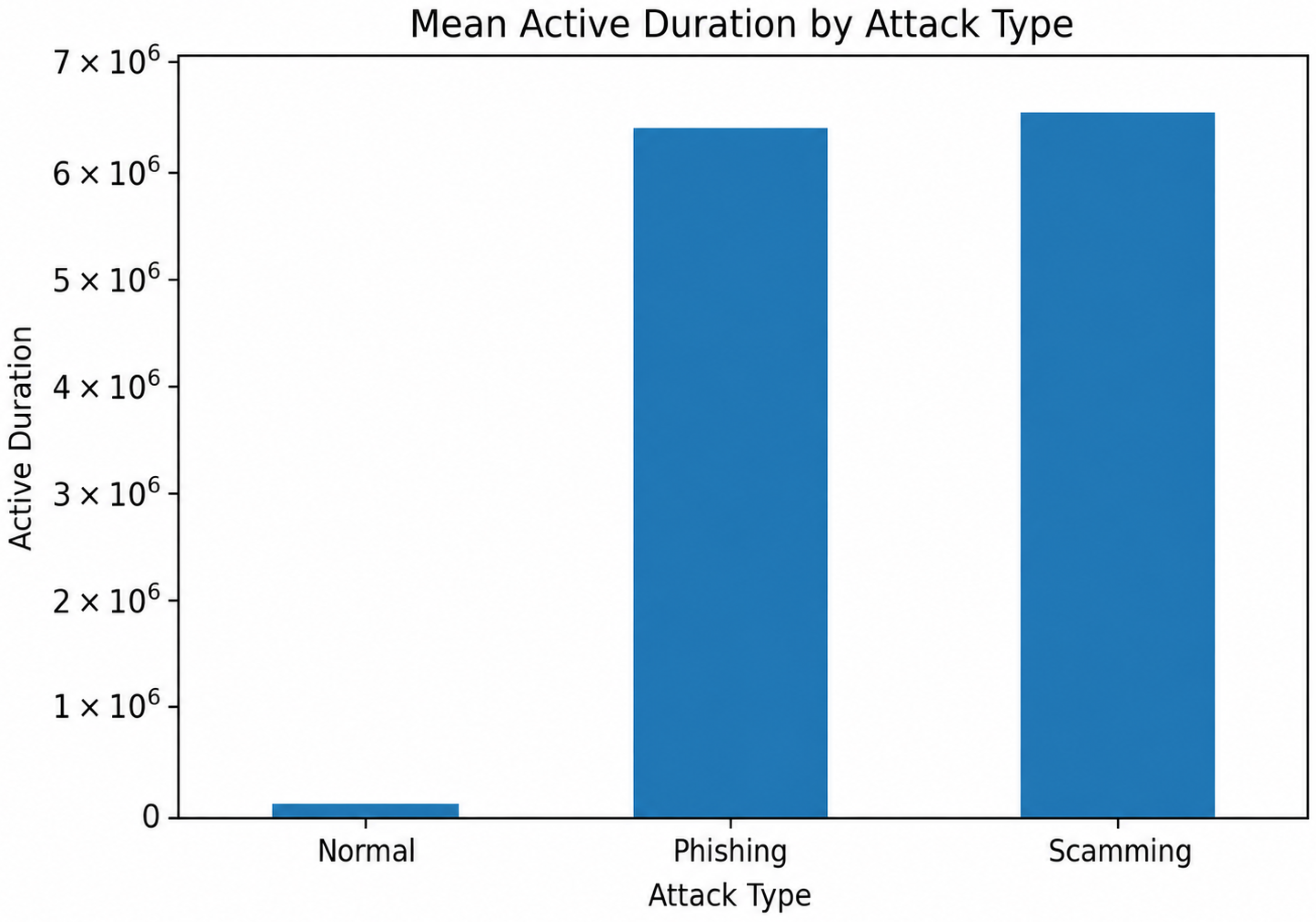
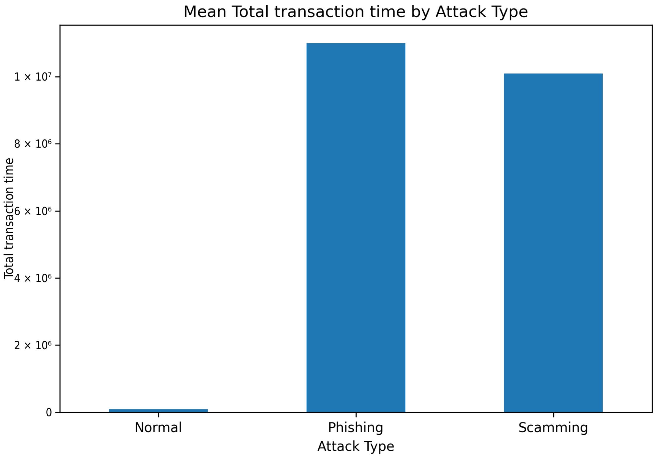
Figure 2 and Figure 3 illustrate the temporal behavior of Ethereum addresses across the three attack categories. These temporal features provide important evidence that fraudulent addresses exhibit longer activity patterns than normal addresses. Figure 2 presents the mean active duration for Normal, Phishing, and Scamming addresses. The results show that Normal addresses have a much shorter average active duration than the two fraudulent classes. In contrast, Phishing and Scamming addresses remain active for substantially longer periods. This suggests that malicious addresses tend to engage in transactions over extended periods, which may reflect repeated interactions, sustained fraudulent campaigns, or prolonged victim-targeting behavior. Therefore, active duration is an important temporal feature for distinguishing fraudulent Ethereum addresses from legitimate ones.
Figure 3 shows the mean total transaction time for each attack category. Similar to the active-duration pattern, the total transaction time for Phishing and Scamming addresses is significantly higher than for Normal addresses. Phishing addresses show the highest total transaction time, followed by Scamming addresses, while Normal addresses exhibit only a minimal value. This indicates that fraudulent addresses are associated with longer cumulative transaction activity, making temporal behavior a useful indicator for multi-class fraud detection. The observed difference also supports the use of graph-based learning models, as temporal persistence combined with neighborhood structure can help identify malicious address behavior more effectively.

3.3. Ethereum Transaction Graph Construction

Since GNNs operate on graph-structured data, the proposed BLTE multi-class dataset was transformed into an Ethereum transaction graph. The graph construction process uses Ethereum addresses as nodes and transaction relationships as directed edges. Let the transaction graph be defined as
G = ( V , E , X , Y ) ,
where V is the set of Ethereum address nodes, E is the set of directed transaction edges, X is the node feature matrix, and Y is the node label vector. Each node v ∈ V represents a unique Ethereum address, and each edge e = ( u , v ) ∈ E represents a transaction relationship from sender address u to receiver address v.
The edge list was generated from the All_fakeAddresses_category transaction records. First, the final node dataset BLTE multi-class was loaded, and the set of valid Ethereum addresses was extracted. The from_address and to_address fields were then normalized using the same preprocessing procedure applied during label construction. Only transaction pairs in which both the sender and receiver addresses were present in the final node set were retained. Duplicate transaction edges were removed to obtain a clean directed edge list. This process produced 6588 directed transaction edges as summarized in Table 6. The generated edge list was saved as BLTE_edges.csv and later converted into the edge_index format required by PyTorch Geometric.
Each node was assigned a feature vector consisting of 23 numerical behavioral attributes:
X v = [ x 1 , x 2 , … , x 23 ] ,
where X v denotes the feature vector of node v. Each node was also assigned a class label:
Y v ∈ N o r m a l , P h i s h i n g , S c a m m i n g .
Unlike traditional machine learning models that treat Ethereum addresses as independent records, the graph representation preserves transaction relationships among addresses. This allows GNN models to aggregate information from neighboring addresses and learn structural dependencies that may indicate fraudulent behavior. Furthermore, the constructed graph enables the proposed models to exploit both node-level behavioral features and graph-level relational patterns. This is particularly important for Ethereum fraud detection because malicious addresses often exhibit abnormal connectivity, repeated interactions, concentrated incoming transactions, prolonged periods of activity, and distinctive gas-usage behavior. Therefore, the proposed graph formulation provides a suitable foundation for learning discriminative embeddings for multi-class Ethereum address classification.

Graph Connectivity Statistics and Handling of Isolated Nodes

Because the transaction graph is highly sparse (6588 directed edges over 73,033 nodes), it is important to characterize how many addresses actually possess transaction neighbors before interpreting the graph learning results. Table 7 reports the connectivity statistics of the constructed graph.
Two observations follow from Table 7. First, the overwhelming majority of addresses (about 88%) are isolated, so for most nodes there is no neighborhood to aggregate. Second, the minority fraud classes are comparatively well connected: most Phishing and Scamming addresses lie in the non-isolated subgraph, which is precisely where message passing can contribute. This distribution explains why graph structure helps the minority classes disproportionately while adding little for the isolated Normal majority.
The way isolated nodes are handled follows directly from the neighborhood-aggregation mechanism shared by all three GNN architectures, defined in Section 3.4. For a node with an empty neighborhood N ( v ) = ⌀ , the neighbor-aggregation term contributes no information, so the update reduces to a learned transformation of the node’s own feature vector (together with the self-representation term). For GraphSAGE, GCN, and GAT alike, an isolated node is therefore embedded essentially as a feed-forward transformation of its own 23 features, which is equivalent to the operation performed by the feature-only MLP baseline. Consequently, for the isolated 88% of the graph, the GNNs and the MLP are expected to behave almost identically, and any genuine graph learning advantage must come from the connected subgraph. This is consistent with the ablation on non-isolated nodes reported in Section 6.6 and directly addresses the concern that, under such sparsity, GNN message passing can degenerate to an MLP for most addresses.

3.4. Graph Neural Network-Based Classification

After constructing the Ethereum transaction graph, the proposed framework applies Graph Neural Network models to perform multi-class node classification. In this task, each Ethereum address is represented as a node, and the objective is to predict the corresponding class label of each node as Normal, Phishing, or Scamming. Unlike traditional machine learning models, which classify each address independently, GNNs exploit both node-level attributes and graph topology by aggregating information from neighboring addresses.
Let the constructed Ethereum graph be represented as G = ( V , E , X , Y ) , where V denotes the set of Ethereum address nodes, E represents the directed transaction edges, X ∈ R | V | × d denotes the node feature matrix, and Y represents the class-label vector. Each node v i ∈ V is associated with a feature vector x i ∈ R d , where d = 23 corresponds to the number of behavioral features used for GNN training. The node classification objective is to learn a mapping function:
f θ : ( X , E ) → Y ,
where f θ denotes the trainable GNN model parameterized by θ . The model learns node embeddings by iteratively aggregating information from neighboring nodes and then uses these embeddings to predict the class label of each Ethereum address.
In this work, three representative GNN architectures were investigated: GAT [9], GCN [10], and GraphSAGE [11]. These models were selected because they represent different message-passing strategies. GAT applies attention mechanisms to assign different importance weights to neighboring nodes, GCN performs convolutional aggregation over graph neighborhoods, and GraphSAGE learns node embeddings through neighborhood sampling and aggregation. The use of these three architectures enables a comparative evaluation of attention-based, convolution-based, and sampling-based graph learning strategies for Ethereum fraud detection.
The models were trained using the same graph structure, node features, and label distribution to ensure a fair comparison. The dataset was divided into training, validation, and testing sets using stratified sampling. Specifically, 70% of the nodes were used for training, 15% for validation, and 15% for testing. Stratified sampling was applied to preserve the distribution of the three classes across all data partitions. Since the dataset is highly imbalanced, class-weighted cross-entropy loss was used during training to reduce the dominance of the Normal class and improve the detection of minority attack classes. The general message-passing operation of a GNN layer can be expressed as
h v ( k ) = σ W ( k ) · AGG ( k ) { h u ( k − 1 ) : u ∈ N ( v ) } ∪ { h v ( k − 1 ) } ,
where h v ( k ) represents the embedding of node v at layer k, N ( v ) denotes the set of neighboring nodes connected to v, W ( k ) is a trainable weight matrix, σ is a nonlinear activation function, and AGG ( k ) denotes the neighborhood aggregation function. Through this process, each node learns a representation that combines its own behavioral features with information from its transaction neighbors. For multi-class prediction, the final node embeddings are passed to a fully connected classification layer followed by a softmax function:
y ^ v = softmax ( W o h v + b o ) ,
where y ^ v denotes the predicted probability distribution over the three classes, W o is the output weight matrix, and b o is the bias term. The predicted class is then obtained as
c ^ v = arg max c ∈ { 0 , 1 , 2 } y ^ v , c ,
where class 0 corresponds to Normal, class 1 corresponds to Phishing, and class 2 corresponds to Scamming. The proposed node-classification framework allows the model to learn fraud-related patterns not only from the individual behavior of each Ethereum address but also from its local transaction neighborhood. This is particularly important in blockchain fraud detection, where malicious addresses often appear in connected communities, share similar transaction patterns, and exhibit abnormal interaction structures. Therefore, GNN-based node classification provides a suitable mechanism for detecting and differentiating between multiple types of malicious Ethereum addresses.

3.5. Explainability Using GNNExplainer

Although GNNs are effective in learning structural and behavioral patterns from transaction graphs, their decision-making process is often difficult to interpret due to the nonlinear aggregation of node features and neighborhood information. In blockchain fraud detection, interpretability is particularly important because security analysts need to understand why a wallet address is classified as Phishing or Scamming. Therefore, this work incorporates an explainability stage using GNNExplainer to provide local explanations for predictions from the trained GNN models.
GNNExplainer [12] is a post hoc explanation method designed to identify the most influential subgraph structures and node features that contribute to a specific GNN prediction. Given a trained model and a target node, GNNExplainer learns a compact explanation by selecting a subset of important edges and feature dimensions that preserve the original prediction as much as possible. In this work, GNNExplainer was applied to the trained GAT, GCN, and GraphSAGE models to analyze how each architecture makes classification decisions for Ethereum addresses. Let f θ denote a trained GNN model, where θ represents the learned model parameters. For a target Ethereum address node v, the model produces a predicted class y ^ v based on the node feature matrix X and the graph edge set E:
y ^ v = f θ ( X , E ) v .
The objective of GNNExplainer is to find an explanation subgraph G S = ( V S , E S ) and a feature mask M X that are sufficient to explain the prediction of node v. The explanation subgraph contains the most relevant neighboring nodes and transaction edges, while the feature mask assigns importance scores to the node attributes. The explanation can be represented as
E v = ( G S , M X ) ,
where E v denotes the explanation generated for node v, G S is the selected explanatory subgraph, and M X is the learned feature-importance mask.
Following the GNNExplainer formulation, the explanation is obtained by maximizing the mutual information between the prediction of the full graph and the prediction conditioned on the explanation subgraph and selected node features:
max G S , M X I ( Y v ; G S , X ⊙ M X ) ,
where I ( · ) denotes mutual information, Y v represents the predicted label of node v, X is the original node feature matrix, M X is the feature mask, and ⊙ denotes element-wise multiplication. This optimization encourages the explainer to identify the smallest, most informative set of features and edges that preserve the model’s prediction.
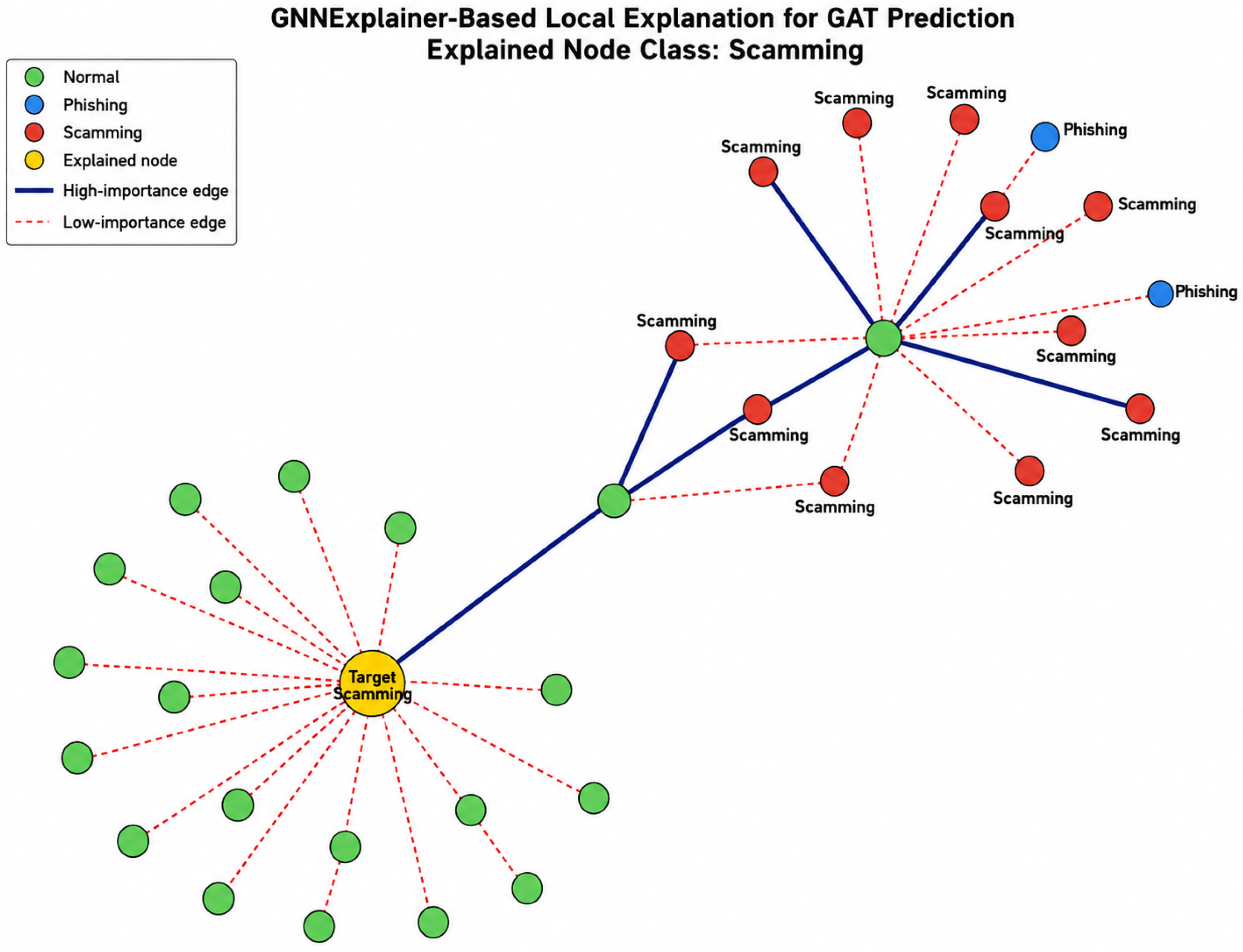
In the proposed framework, GNNExplainer was applied after model training and evaluation. For each trained architecture, a correctly classified malicious node was selected from the test set, with preference given to the Scamming class, as it represents high-risk fraudulent behavior. The selected node was then explained using a two-hop neighborhood to capture local transaction dependencies around the target address. This setting allows the analysis to consider both direct and indirect transactional relationships that may contribute to fraud classification.
The output of GNNExplainer consists of two main components. First, an edge-importance mask is generated to identify the transaction relationships that most strongly influenced the prediction. Edges with higher importance scores indicate stronger contribution to the model decision. Second, a node-feature importance mask is produced to determine which behavioral attributes contributed most to the classification outcome. These attributes include connectivity-based features, transaction amount features, temporal activity features, and gas-related features.
For visualization, the explanation subgraph was plotted by highlighting the target node, malicious neighboring nodes, normal neighboring nodes, and important transaction edges. The target node was marked distinctly, while the remaining nodes were colored according to their class labels: Normal, Phishing, and Scamming. Edge thickness was scaled according to the learned edge-importance score, where thicker edges indicate a stronger influence on the GNN prediction. In addition, the top-ranked node features were visualized as a feature-importance bar chart for each model.
The use of GNNExplainer provides two important benefits in this study. First, it improves the transparency of the proposed Ethereum fraud detection framework by revealing which graph relationships and node attributes drive model predictions. Second, it enables a qualitative comparison between GAT, GCN, and GraphSAGE. Specifically, the explanation subgraphs reveal whether each model relies on broad neighborhood structures, compact local patterns, or attention-driven interactions. This allows the performance results to be interpreted not only quantitatively through accuracy and F1-score but also qualitatively through the structural and feature-level evidence used by each model.

3.6. Performance Evaluation

The performance of the proposed Ethereum fraud detection framework was evaluated using both quantitative classification metrics and visual diagnostic analyses. Since the BLTE multi-class dataset is highly imbalanced, with the Normal class representing the majority of samples and the Phishing and Scamming classes representing minority fraud categories, accuracy alone is insufficient to assess model effectiveness. Therefore, several complementary metrics were used, including accuracy, precision, recall, Macro-F1 score, weighted F1-score, confusion matrix analysis, and training/validation loss curves.
The dataset was divided into training, validation, and testing subsets using a stratified sampling strategy. Specifically, 70% of the nodes were used for training, 15% for validation, and 15% for testing. Stratification was applied to preserve the original class distribution across the three subsets. The training set was used to optimize the model parameters, the validation set was used to monitor generalization during training, and the test set was used only for final performance reporting.
Let C denote the number of classes, where C = 3 for the proposed classification task: Normal, Phishing, and Scamming. For each class c, the classification results are represented using true positives ( T P c ) , false positives ( F P c ) , false negatives ( F N c ) , and true negatives ( T N c ) . Accuracy measures the proportion of correctly classified nodes among all test nodes and is defined as [19]
A c c u r a c y = ∑ c = 1 C T P c N
where N denotes the total number of test nodes. Precision measures the proportion of nodes predicted as a given class that are actually correct. For class c [20], precision is calculated as
P r e c i s i o n c = T P c T P c + F P c .
Recall measures the proportion of actual nodes from class c that were correctly identified by the model [21]. It is calculated as
R e c a l l c = T P c T P c + F N c .
The F1-score provides a harmonic mean between precision and recall and is particularly useful when the dataset is imbalanced. For each class c [22], it is computed as
F 1 c = 2 × P r e c i s i o n c × R e c a l l c P r e c i s i o n c + R e c a l l c .
To evaluate balanced performance across all classes, the Macro-F1 score was used. Macro-F1 assigns equal importance to each class regardless of its sample size and is therefore suitable for assessing the model’s ability to detect minority attack classes, which is defined as [23]
M a c r o - F 1 = 1 C ∑ c = 1 C F 1 c .
In addition, the weighted F1-score was used to account for class support. Unlike Macro-F1, weighted F1 considers the number of samples in each class and is calculated as [24]
W e i g h t e d - F 1 = ∑ c = 1 C n c N F 1 c ,
where n c denotes the number of test samples belonging to class c. During training, the categorical cross-entropy loss was used as the optimization objective. Because of the severe class imbalance in the dataset, class weighting was applied to reduce the dominance of the majority Normal class and encourage the model to learn from minority fraudulent classes. The weighted cross-entropy loss is defined as [25]
L = − ∑ c = 1 C w c y c log ( y ^ c ) ,
where w c is the class weight for class c, y c is the ground-truth label indicator, and y ^ c is the predicted probability for class c. The performance of GAT, GCN, and GraphSAGE was compared under identical experimental settings. For each model, the training and validation accuracy curves were analyzed to assess learning progress, while the loss curves were used to monitor convergence behavior. The Macro-F1 curves were examined to evaluate the model’s ability to learn minority classes during training. Finally, the test-set classification report and confusion matrix were used to compare final predictive performance.
The combination of these metrics provides a comprehensive assessment of model performance. Accuracy and weighted F1-score indicate the overall predictive capability of the model, while Macro-F1, precision, and recall provide deeper insight into minority-class detection. This is essential for Ethereum fraud detection, where correctly identifying rare malicious addresses is more important than simply achieving high overall accuracy on the dominant Normal class.

4. Experimental Setup

This section describes the implementation environment, model configurations, and training protocol used to evaluate the three Graph Neural Network architectures. All models were implemented and evaluated under identical conditions to ensure a fair comparison.

4.1. Implementation Environment

The proposed framework was implemented in Python 3.10 using PyTorch 2.0.1 and PyTorch Geometric 2.3.1 for graph construction and GNN training. Auxiliary data processing was performed using pandas, NumPy, and scikit-learn, and GNNExplainer was applied using the implementation provided in PyTorch Geometric. All experiments were conducted on an NVIDIA RTX 3090 GPU with 24 GB of memory, running Ubuntu 22.04.

4.2. Model Architectures

Each architecture was configured as a two-layer message-passing network followed by a fully connected softmax classification layer. The hidden dimension was set to 64 units, and the ReLU activation function was applied between layers. A dropout rate of 0.5 was used to mitigate overfitting. For the GAT model, 8 attention heads were employed in the first layer, while GraphSAGE used the mean aggregator for neighborhood aggregation. Unless otherwise stated, all three models shared the same hidden dimension and depth so that performance differences are attributable to the underlying message-passing mechanism rather than to differences in model capacity.

4.3. Training Configuration

All models were trained for 300 epochs using the Adam optimizer with a learning rate of 0.01 and a weight decay of 5 × 10 − 4 . Training was performed using full-batch updates over the entire graph. To address the severe class imbalance, a class-weighted cross-entropy loss was used, with class weights set inversely proportional to class frequency. Following the protocol described in Section 3, the dataset was partitioned into training (70%), validation (15%), and testing (15%) subsets using stratified sampling to preserve the class distribution across all partitions. The key hyperparameters are summarized in Table 8.

4.4. Robustness, Baseline, and Significance-Testing Protocol

It is sufficient for the exact Wilcoxon signed-rank test to reach the significance levels reported below, and it keeps the full seven-model × ten-seed training budget tractable on a single GPU; the accompanying per-seed values are provided in Appendix B so that the stability of each estimate can be inspected directly.
Classical baselines are included to determine whether graph message passing provides an improvement beyond strong feature-based learners. The baseline suite contains a feature-only multilayer perceptron (MLP), Random Forest (RF) [26], and XGBoost [27]. RF and XGBoost use the same 23 address-level features used by the GNNs but discard the edge set. A re-implemented published GNN-style comparator is also included by adapting the Chebyshev graph-convolution baseline used in Ethereum phishing detection by Li et al. [14]. Table 9 summarizes the models to be included in the robustness extension.
For statistical testing, the primary comparison used paired per-seed macro F1-scores, because the same random seeds and split-generation procedure are shared across models. The non-parametric Wilcoxon signed-rank test [28] was used for the paired model comparisons, as normality of the paired differences cannot be assumed at K = 10 ; it was computed in its exact form for the ten matched pairs rather than the normal approximation. When several pairwise tests were reported, the p-values were adjusted using the Holm–Bonferroni procedure [29]. The main confirmatory comparisons were GraphSAGE versus MLP, RF, XGBoost, Chebyshev GCN, GAT, and GCN. Following Demšar [30], each test is interpreted together with a matched-pairs rank-biserial effect size and a 95 % confidence interval for the macro-F1 difference, rather than by p-values alone.
In addition to aggregate metrics, absolute-count confusion matrices are reported using the class order Normal, Phishing, and Scamming, both for a representative split and summed across the ten seeds (Section 6.2). This is necessary because percentage-normalized heat maps can hide the small number of minority-class examples in the test partition. For the construct-validity threat associated with edge construction, an additional label-independent graph was reconstructed from transaction pairs obtained without using attack-category fields, and the same node labels and features were evaluated on that label-independent edge set (Section 6.3). As reported there, the GraphSAGE advantage persists but decreases under the reconstructed edge set, so the structural contribution is interpreted cautiously and the behavioral node features are treated as the dominant source of predictive signal.

5. Results and Discussion

This section presents the experimental evaluation of three Graph Neural Network architectures, namely GAT, GCN, and GraphSAGE, for Ethereum wallet attack detection using the BLTE multi-class dataset. The objective was to classify Ethereum addresses into three categories: Normal, Phishing, and Scamming. The models were trained using identical graph structures and node features to ensure a fair comparison. Their performance was evaluated using accuracy, loss, Macro-F1 score, confusion matrices, and explainability analysis based on GNNExplainer. The comparative results demonstrate notable differences in the learning capabilities of the investigated GNN architectures.

5.1. Performance Analysis of the GAT Model

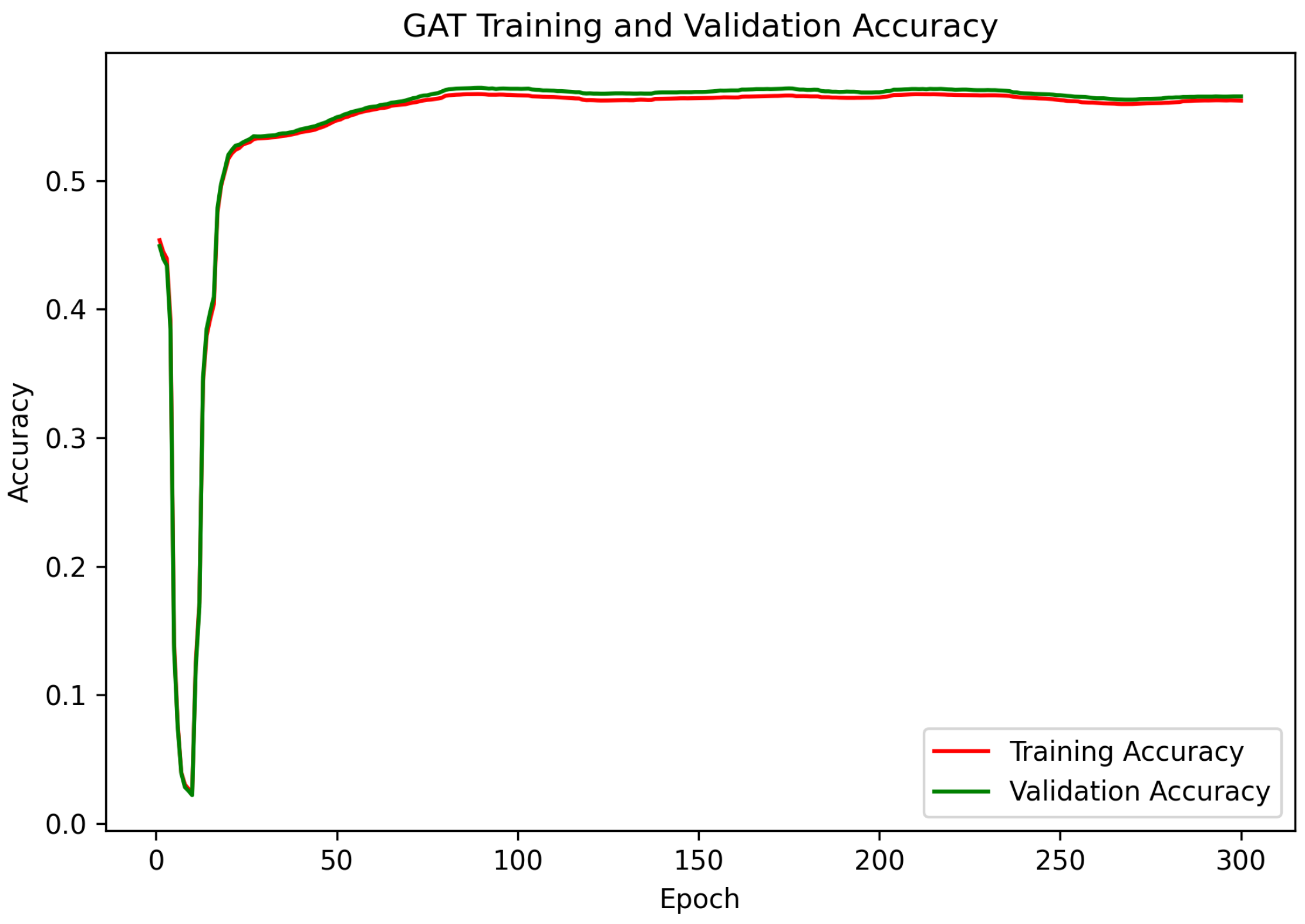
The performance of the Graph Attention Network is illustrated in Figure 4, Figure 5, Figure 6, Figure 7 and Figure 8. As shown in Figure 4, the training and validation accuracy curves increased rapidly during the early stages of training and reached a peak value of approximately 58%. After approximately 150 epochs, a slight performance decline was observed, resulting in a final validation accuracy of approximately 55%.
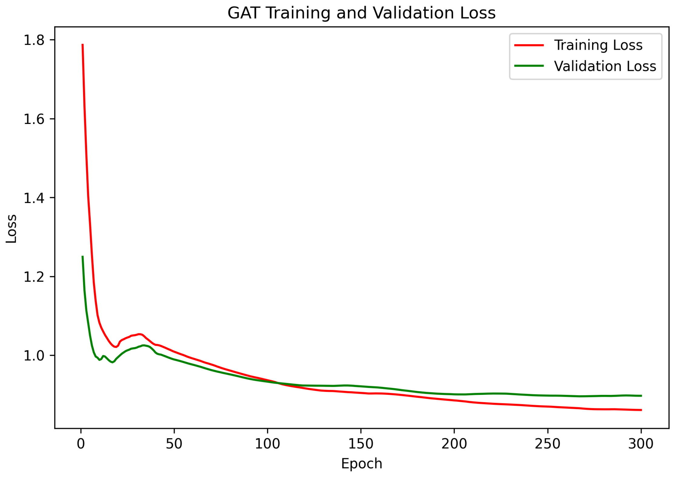
The loss curves shown in Figure 5 demonstrate a gradual reduction in both training and validation loss throughout the optimization process. The training loss decreased from approximately 1.07 to 0.84, while the validation loss decreased from approximately 0.99 to 0.88. Although the optimization process remained stable, the achieved loss values were noticeably higher than those observed with GraphSAGE and GCN, indicating weaker representation-learning capability.
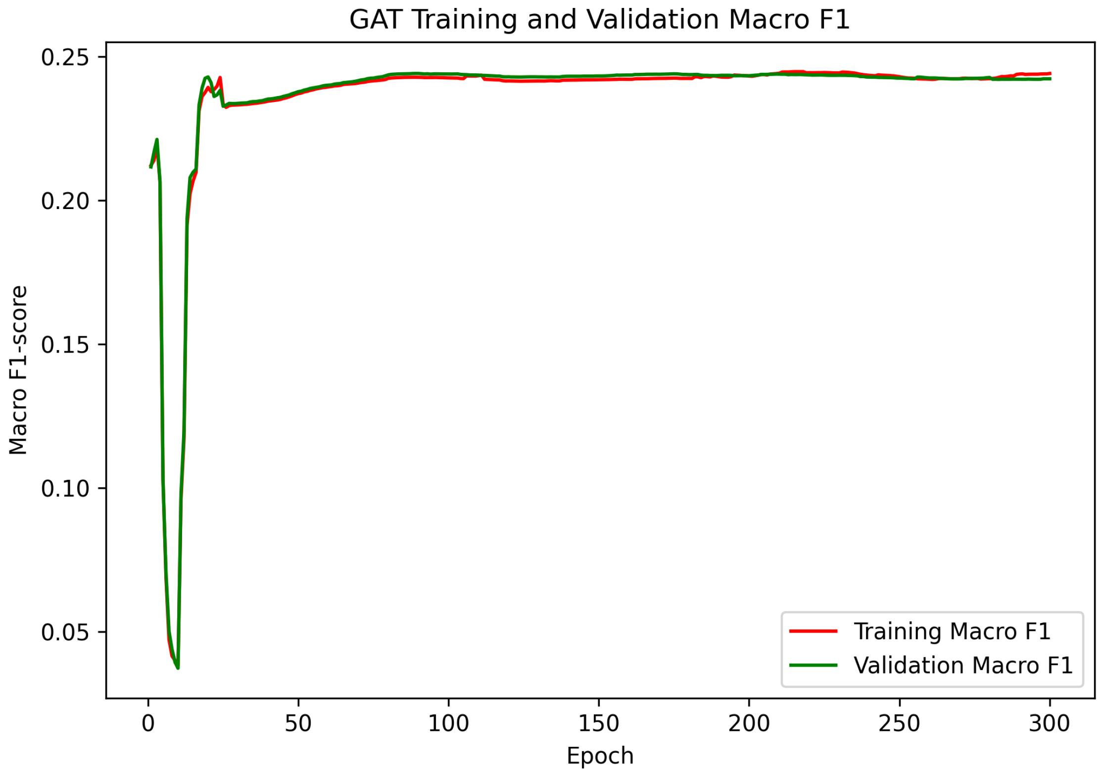
The Macro-F1 score evolution shown in Figure 6 further confirms this limitation. The score peaked near 0.26 and gradually stabilized around 0.24. Compared with the values achieved by GCN and GraphSAGE, the significantly lower Macro-F1 score suggests that the attention mechanism was unable to effectively separate Normal, Phishing, and Scamming wallets within the transaction graph.
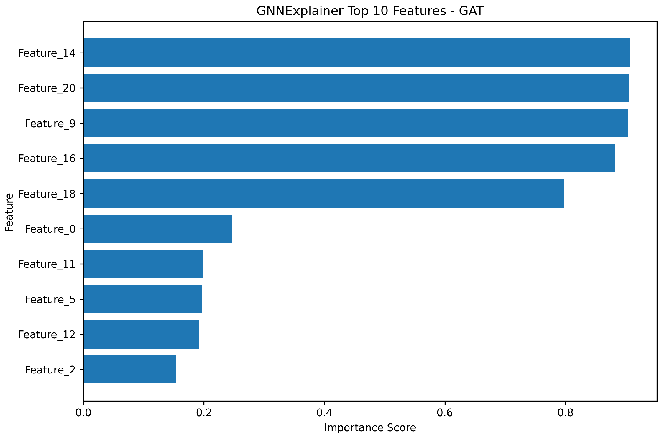
The GNNExplainer-based explanation shown in Figure 7 indicates that GAT relied on a broader set of neighboring nodes containing both malicious and legitimate addresses. Unlike GraphSAGE, which focused on highly localized structures, GAT distributed attention across multiple neighboring nodes. The feature importance ranking shown in Figure 8 identifies Features 14, 20, 9, 16, and 18, corresponding to Avg time outgoing, Min time interval, Max amount incoming, Active Duration, and Mean time interval, as the most influential attributes. Although these features received high attention scores, their contribution did not translate into superior classification performance.
One possible explanation is that the Ethereum transaction graph contains noisy and heterogeneous neighborhood relationships. Consequently, the attention mechanism may assign importance to irrelevant neighbors, resulting in suboptimal aggregation and reduced predictive accuracy.

5.2. Performance Analysis of the GCN Model

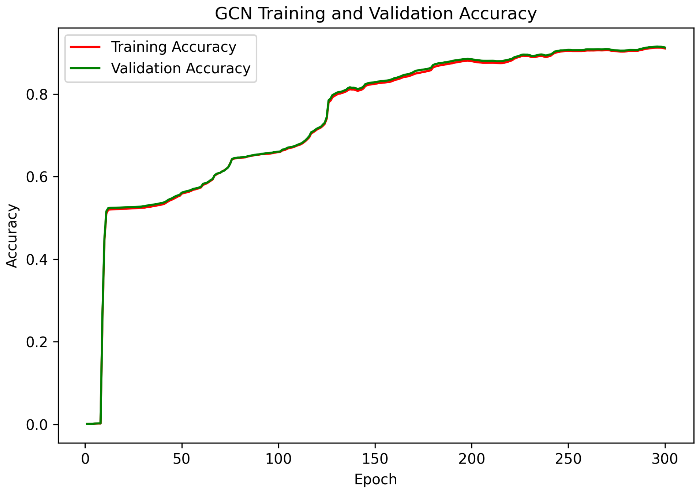
The training and validation accuracy curves of the GCN model are presented in Figure 9. The model exhibited stable learning behavior throughout the training process. Initially, both training and validation accuracy were approximately 39%, then gradually increased as training progressed. After 300 epochs, the validation accuracy reached approximately 87%, while the training accuracy converged near 86%. The close overlap between the two curves indicates that the model generalized well to unseen data and did not suffer from severe overfitting.
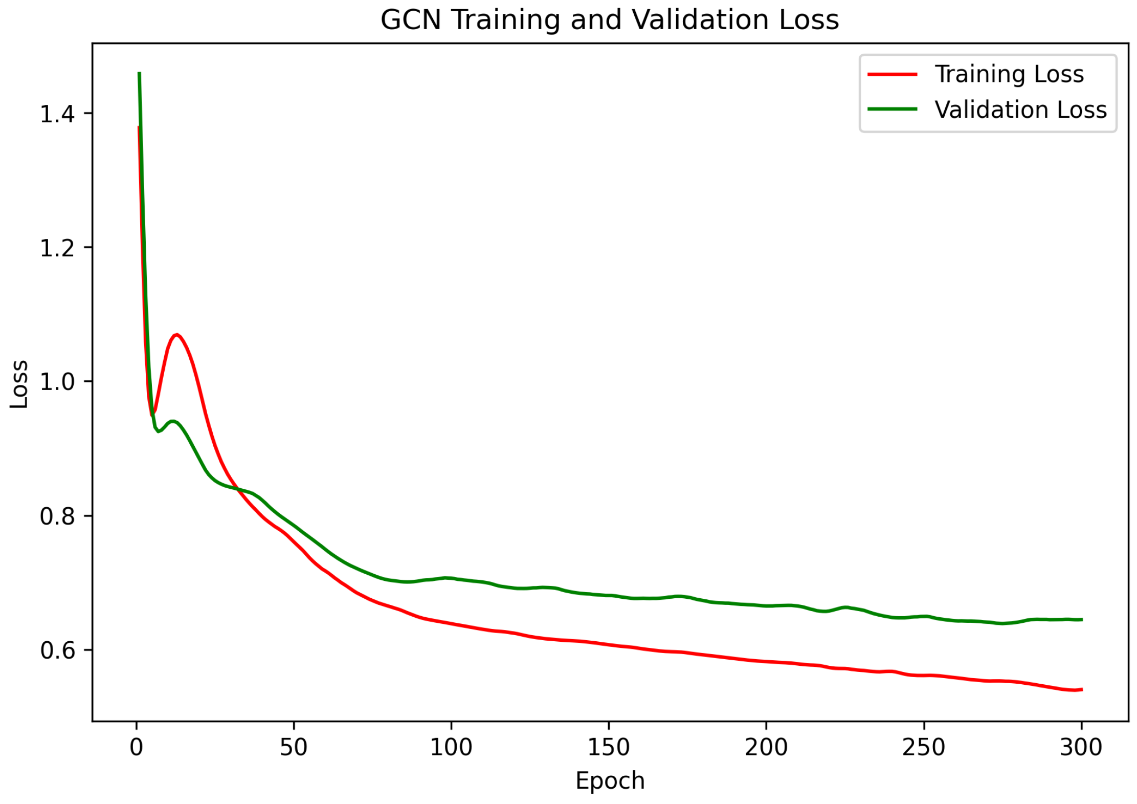
The corresponding training and validation loss curves are shown in Figure 10. The training loss decreased steadily from approximately 1.15 to 0.55, whereas the validation loss decreased from approximately 0.91 to 0.65. The smooth reduction of both curves demonstrates successful optimization and effective learning of graph representations. Furthermore, the relatively small difference between training and validation loss suggests that the model maintained good generalization throughout the learning process.
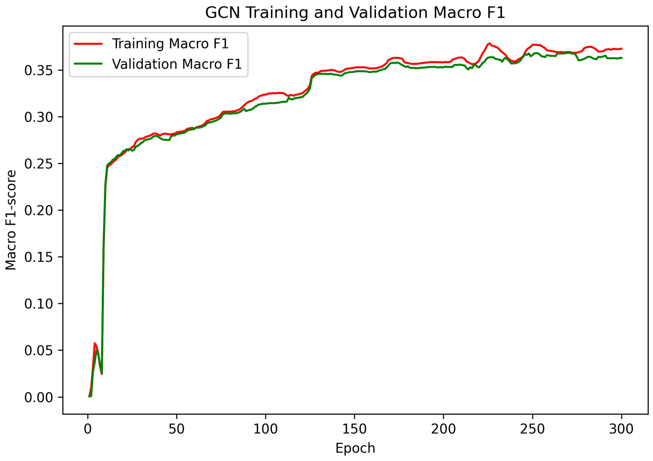
The Macro-F1 score evolution shown in Figure 11 provides additional insight into multi-class classification performance. The score increased from approximately 0.22 at the beginning of training to around 0.38 at convergence. Although the model achieved relatively high classification accuracy, the Macro-F1 score remained noticeably lower. This observation indicates that the model was more effective at identifying the majority class than minority attack classes, a common challenge in blockchain fraud detection datasets characterized by class imbalance.
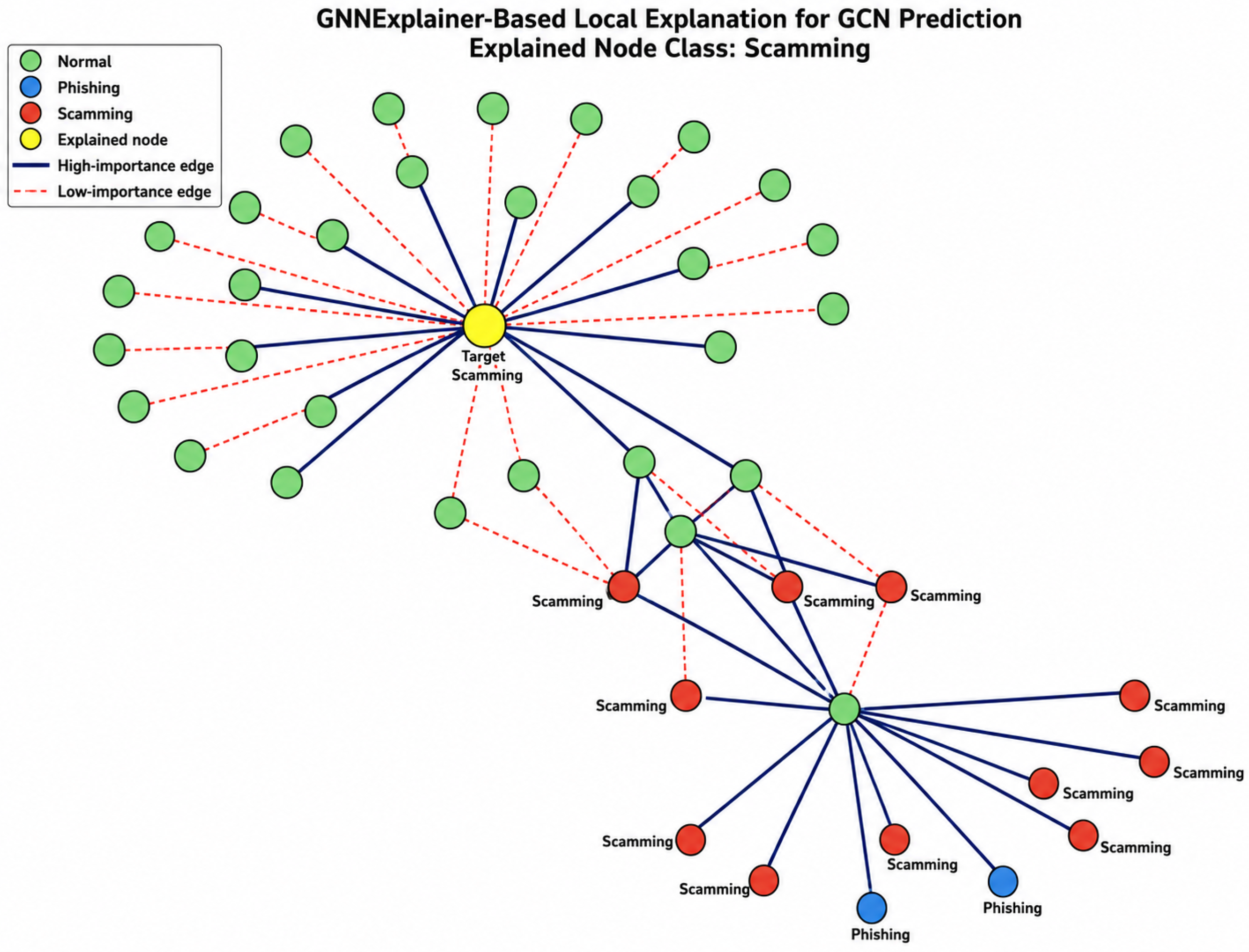
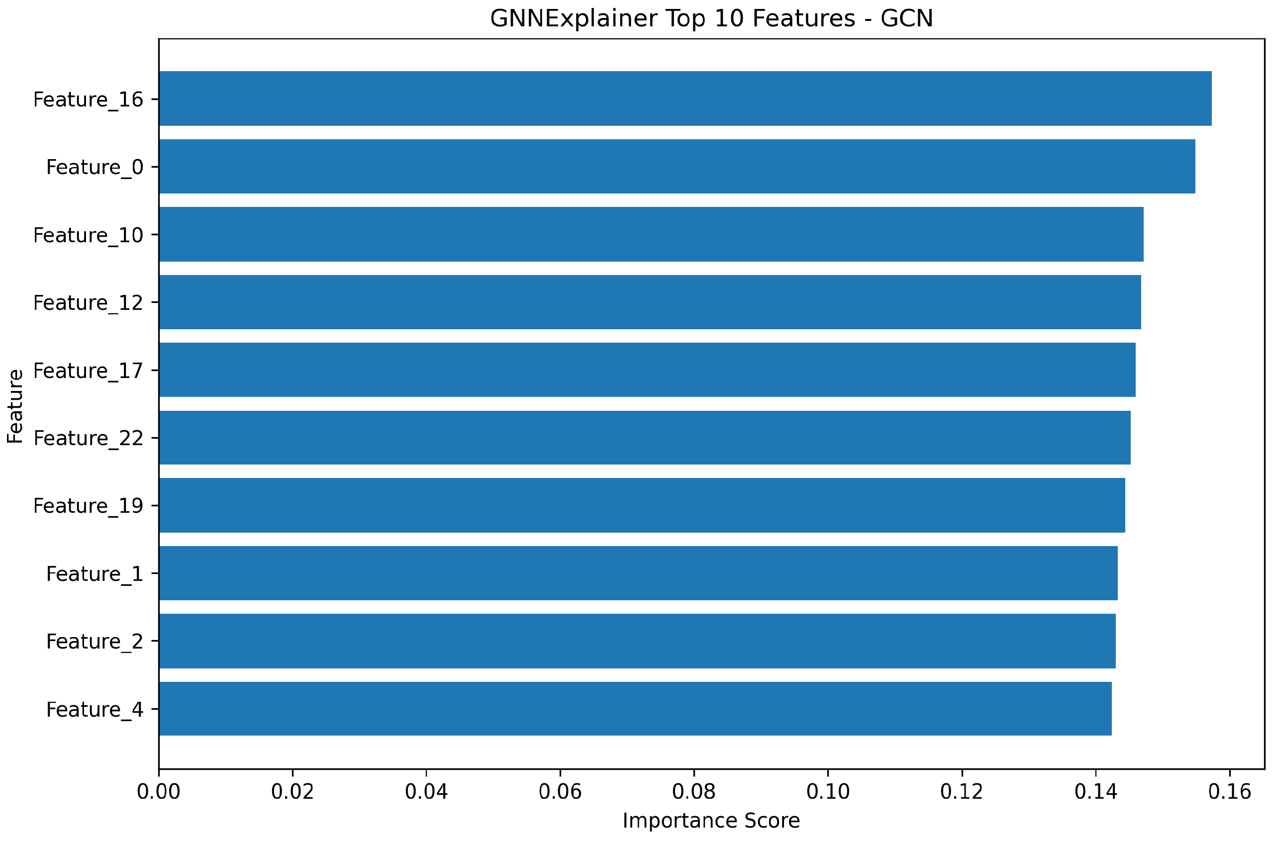
To further understand the prediction mechanism, GNNExplainer was applied to generate local explanations. The explanation subgraph presented in Figure 12 reveals that the GCN model relied on a relatively large neighborhood structure containing interconnected Normal, Phishing, and Scamming nodes. This behavior indicates that GCN primarily exploits multi-hop message propagation and global graph connectivity when making classification decisions. The feature importance analysis shown in Figure 13 identifies Features 16, 0, 10, 12, and 17, corresponding to Active Duration, all_degree, Max amount outgoing, Min amount outgoing, and Clustering coefficient, as the most influential attributes contributing to the classification process. The relatively balanced distribution of feature importance suggests that the model leveraged multiple transactional characteristics simultaneously rather than depending heavily on a single feature.
Overall, the GCN model demonstrated strong learning capability and stable convergence behavior. However, its moderate Macro-F1 score and relatively high number of false-positive predictions indicate limitations in capturing fine-grained behavioral patterns associated with malicious wallet activities.

5.3. Performance Analysis of the GraphSAGE Model

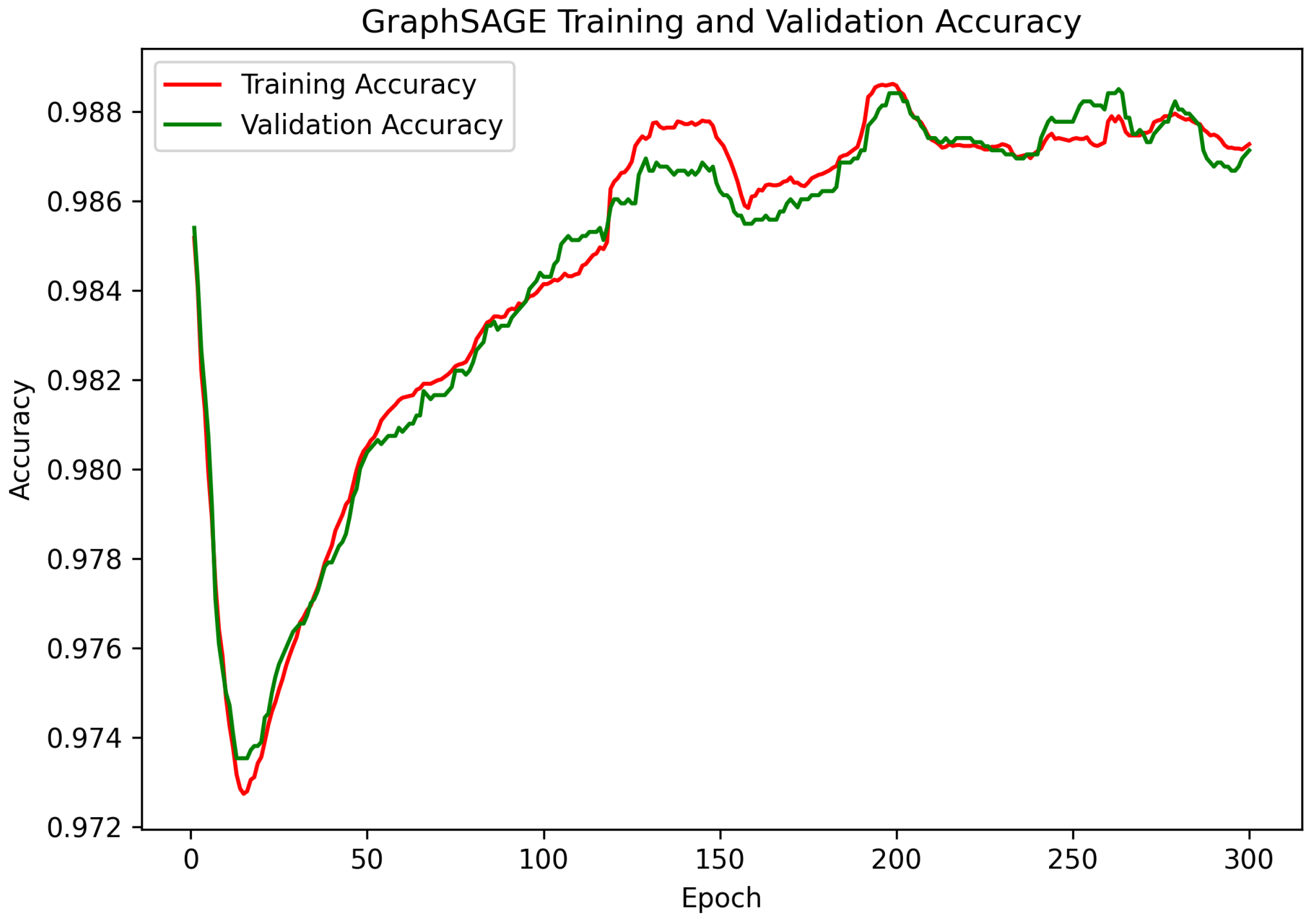
The training and validation accuracy curves for GraphSAGE are presented in Figure 14. Compared with GCN, GraphSAGE exhibited significantly faster convergence and achieved remarkably higher classification performance. The validation accuracy increased rapidly during the first 30 epochs and subsequently stabilized near 99%. The nearly identical training and validation curves indicate excellent generalization capability and demonstrate that GraphSAGE successfully learned highly discriminative graph representations.
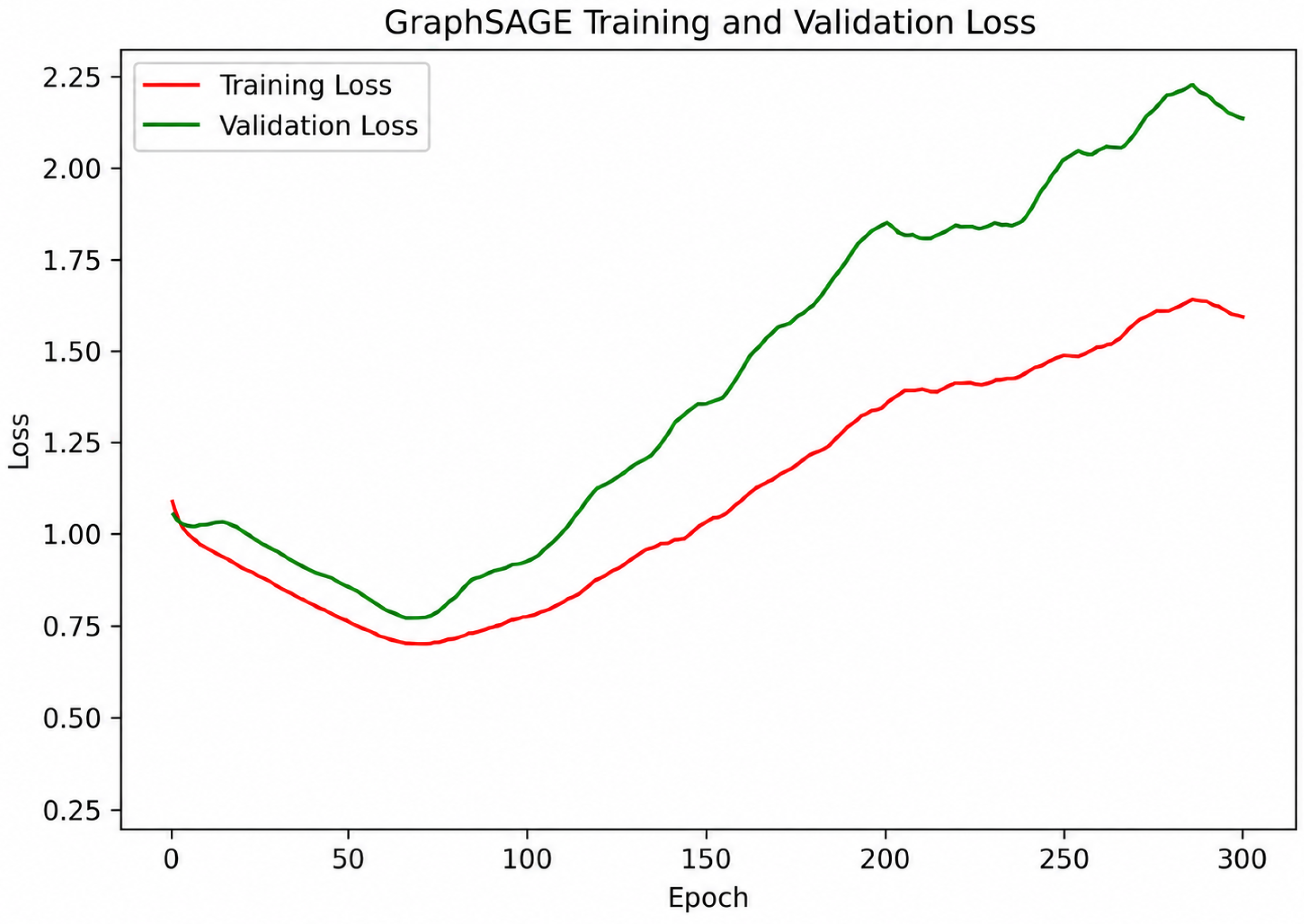
The training and validation loss curves shown in Figure 15 provide a more refined analytical perspective. Both curves decreased during the early training epochs, indicating that GraphSAGE initially learned useful representations from the node features and local graph structure. However, after the initial convergence phase, both the training loss and validation loss began to increase, while the validation accuracy remained extremely high. This behavior suggests increasing model confidence rather than uniformly improved generalization, and it may indicate mild overfitting or overconfidence under severe class imbalance.
Because overall accuracy is dominated by the majority Normal class, it can remain high even when the model becomes less well calibrated on the rare fraudulent classes. Therefore, the loss behavior in Figure 15 should be interpreted together with macro-level metrics, confusion matrices, and the multi-seed evaluation reported in Section 6.1, rather than relying on headline accuracy alone.
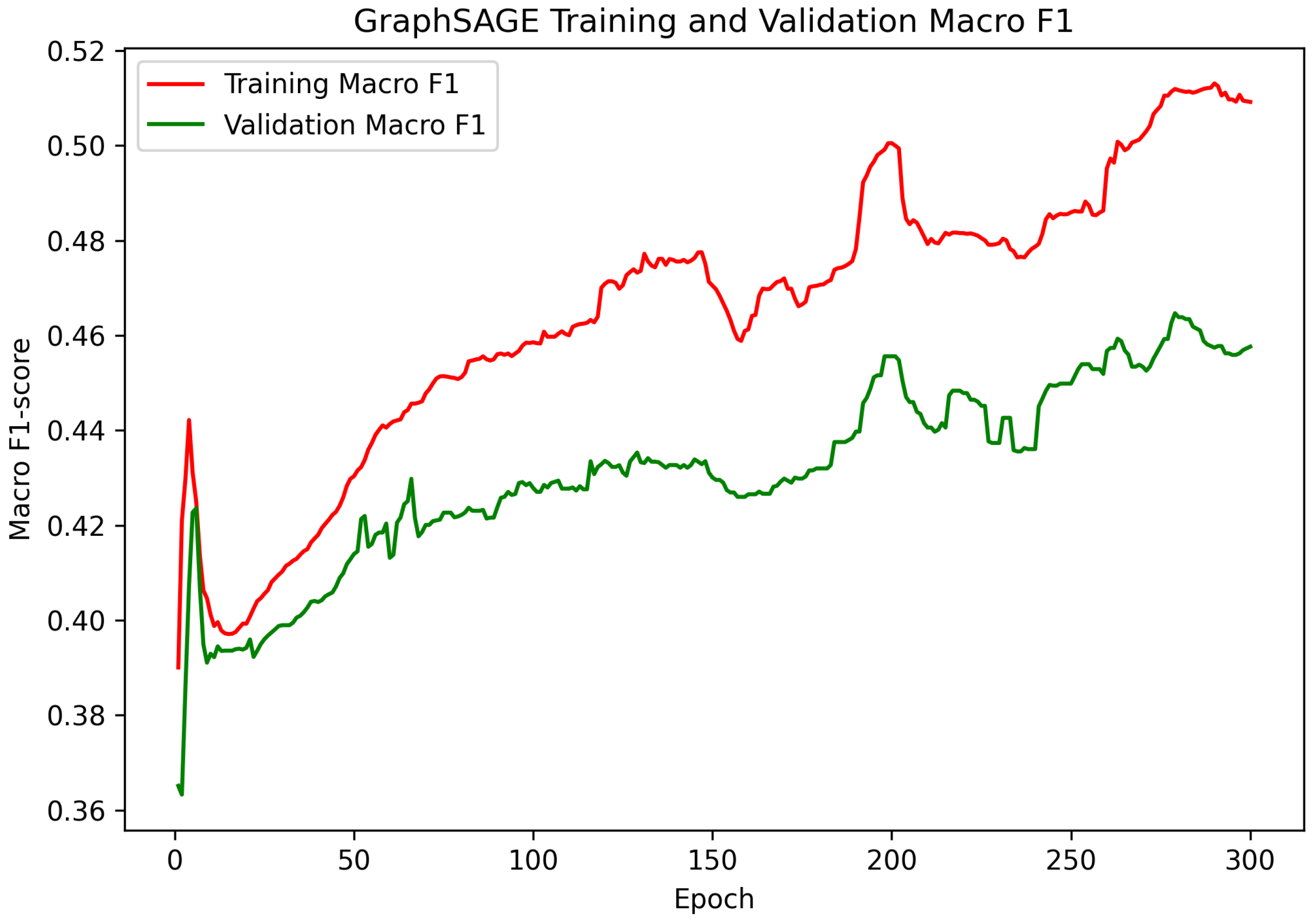
The Macro-F1 score progression illustrated in Figure 16 further supports the effectiveness of GraphSAGE for the multi-class classification task. The validation macro-F1 score increased to approximately 0.46–0.48 and remained higher than the corresponding validation scores obtained by GCN and GAT. This improvement indicates that GraphSAGE learned more useful representations for the minority attack classes than the other implemented GNN architectures, although the absolute macro-F1 value still reflects the difficulty of balanced classification under severe class imbalance.
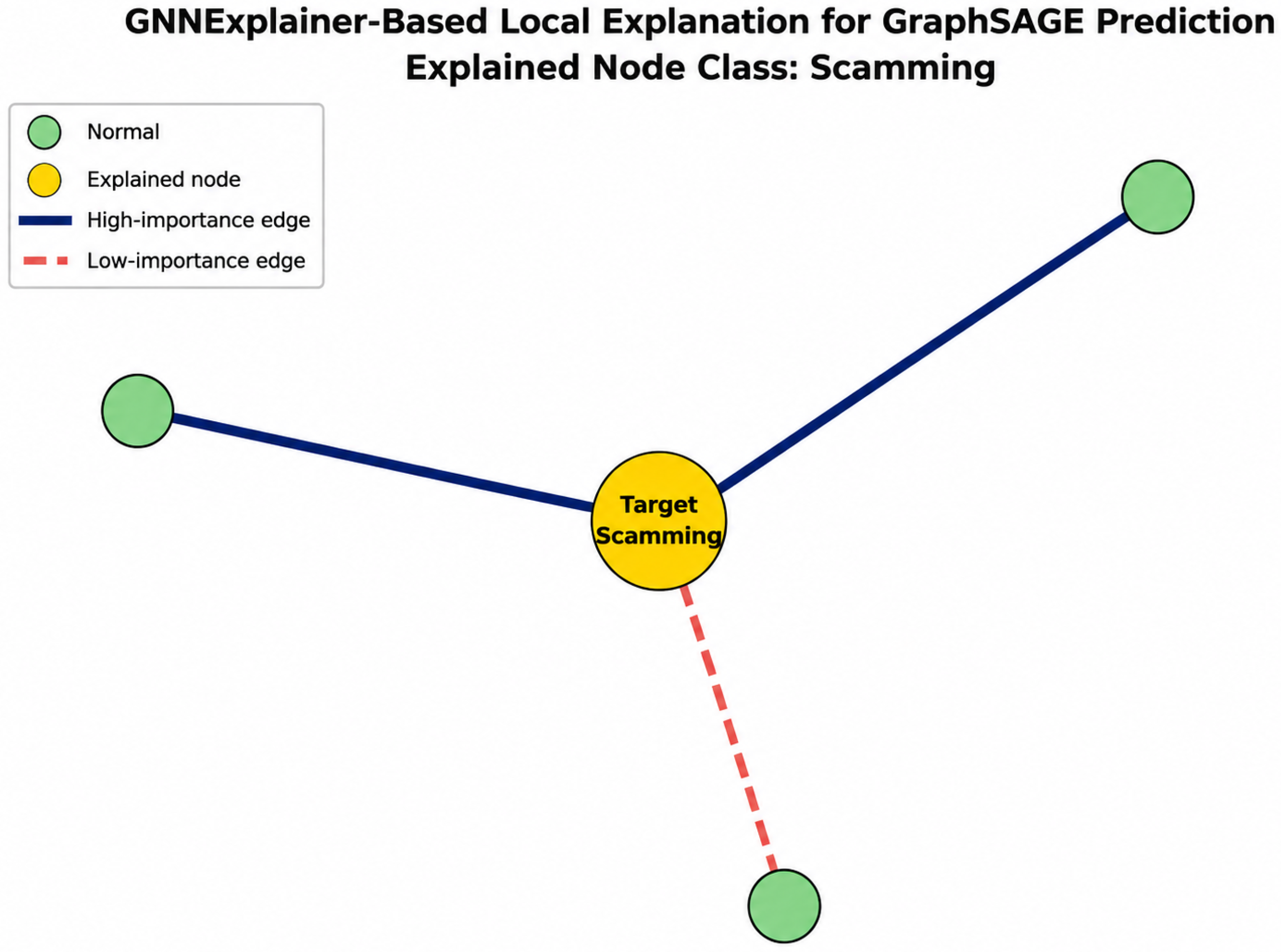
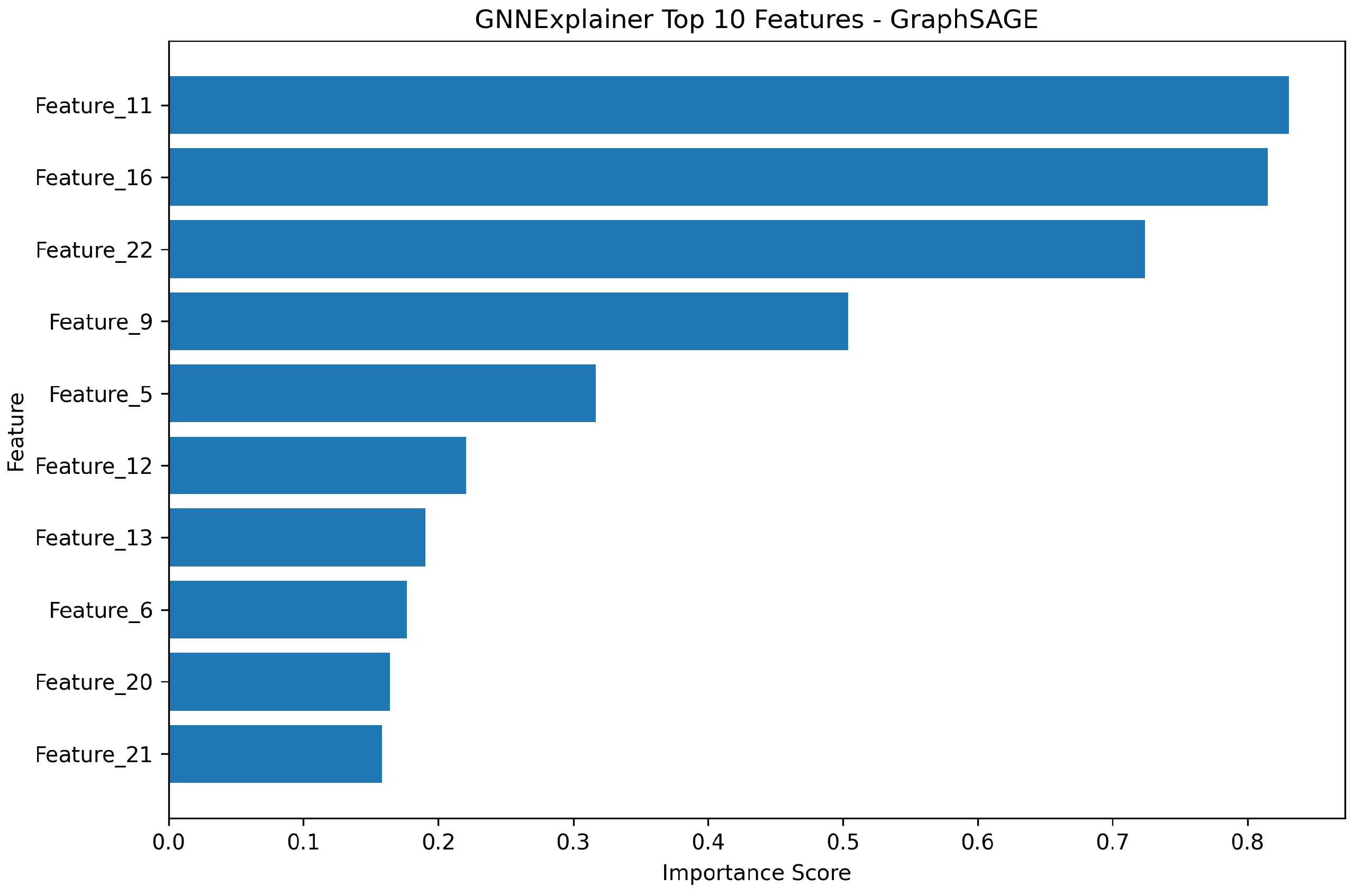
The explanation generated by GNNExplainer is illustrated in Figure 17. Unlike the large explanation subgraph observed in GCN, GraphSAGE relied on a highly localized neighborhood structure comprising only a few influential nodes. This finding suggests that GraphSAGE successfully learned compact and meaningful local patterns associated with fraudulent activities. The feature importance ranking shown in Figure 18 reveals that Features 11, 16, 22, and 9, corresponding to Min amount incoming, Active Duration, Avg gas limit, and Max amount incoming, were the most influential attributes driving the classification decisions. The significantly higher importance scores for these features indicate that GraphSAGE focused on a smaller set of highly discriminative characteristics.
The superior performance of GraphSAGE can be attributed to its neighborhood sampling and aggregation mechanism, which effectively captures local graph structures while preventing excessive smoothing of node representations. Since fraudulent Ethereum wallets often interact within localized transaction communities, GraphSAGE appears particularly well suited for modeling such behavior.

6. Comparative Evaluation of GNN Models

To comprehensively evaluate the effectiveness of graph-based DL for Ethereum address classification, three representative Graph Neural Network architectures, namely GAT, GCN, and GraphSAGE, were implemented and assessed using the BLTE multi-class dataset. The models were trained using identical graph representations, feature sets, and data partitions to ensure a fair comparison. Performance was evaluated using classification accuracy, macro-level precision, macro-level recall, macro-level F1-score, and weighted F1-score.
The quantitative comparison presented in Table 10 demonstrates clear differences in the predictive capabilities of the three architectures. Among the evaluated models, GraphSAGE achieved the highest overall performance with an accuracy of 98.87%, a macro precision of 45.24%, a macro recall of 80.75%, and a macro F1-score of 51.12%. In contrast, GCN achieved an accuracy of 85.07% and a macro F1-score of 39.27%, while GAT produced the lowest performance with an accuracy of 53.50% and a macro F1-score of 25.28%. These results indicate that GraphSAGE is more effective at capturing neighborhood information and preserving discriminative structural patterns within the Ethereum transaction graph. The values in Table 10 correspond to a single stratified split and are reported for illustration only; the primary, statistically defensible comparison is the ten-seed evaluation in Section 6.1 (Table 11), and every confirmatory claim in this paper relies on that repeated-seed protocol rather than on the single split.

6.1. Multi-Seed, Baseline, and Significance Results

To assess whether the single-run results in Table 10 are stable across random initialization and data partitioning, all models were evaluated over ten stratified random seeds. The repeated evaluation included three feature-based classical baselines, namely multilayer perceptron (MLP), Random Forest [26], and XGBoost [27], in addition to a re-implemented graph baseline based on Chebyshev graph convolution. The same node features, class encoding, class-imbalance handling where applicable, and train/validation/test proportions were used across all runs. Table 11 reports mean ± standard deviation values over the ten seeds.
The multi-seed results preserve the general trend observed in the single-run experiment. GraphSAGE achieved the highest macro recall and macro F1-score among the evaluated models, while the feature-only MLP remained a strong comparator and approached the GraphSAGE result. This indicates that the behavioral address features carry substantial discriminative information and that the graph component provides an additional, but modest, improvement. Therefore, the performance claim should be interpreted as evidence that GraphSAGE provides the best mean macro-level performance under the repeated-seed protocol, rather than as a large-margin improvement over all feature-based baselines. In particular, the paired significance tests show that GraphSAGE is significantly higher than GAT, GCN, Random Forest, XGBoost, and Chebyshev GCN, but its difference from the MLP baseline is not statistically significant after Holm correction.
To test whether the observed macro-F1 differences were robust, paired Wilcoxon signed-rank tests [28] were applied to the per-seed macro-F1 values using GraphSAGE as the reference model. Holm correction [29] was then used to control the family-wise error rate across the six pairwise comparisons, following standard recommendations for classifier comparison [30]. Table 12 reports the adjusted p-values.
The complete per-seed macro-F1 values that underlie these tests are listed in Appendix B to make the estimates fully inspectable and the confidence intervals reproducible.

6.2. Absolute-Count Confusion Matrices

Because the BLTE multi-class dataset is extremely imbalanced, percentage-normalized confusion matrices can hide the small number of minority-class test samples. Therefore, Table 13 reports absolute-count confusion matrices for the principal models using the class order Normal, Phishing, and Scamming, for a single representative stratified test split containing 10,930 Normal, 10 Phishing, and 15 Scamming addresses. To avoid drawing conclusions from one split, Table 14 then reports per-class precision, recall, and F1-score as mean ± standard deviation over the ten seeds, and Table 15 reports the confusion-matrix counts summed over the ten held-out test partitions.
The absolute counts clarify the interpretation of the aggregate metrics. GraphSAGE correctly identifies a larger fraction of the Phishing and Scamming addresses than the competing GNNs, but it also produces minority-class false positives among Normal addresses. Consequently, its macro recall is relatively strong, while macro precision and macro F1 remain limited. This pattern is expected under the extreme class imbalance and confirms that high accuracy and weighted F1-score should not be interpreted as sufficient evidence of minority-class detection quality.
The high headline accuracy (98–99%) and weighted F1-score (around 0.99) reported for the strongest models are indeed misleading as indicators of fraud detection quality, because the Normal class constitutes 99.77% of the data and therefore dominates both metrics: a trivial classifier that labels every address Normal would already reach roughly 99.77% accuracy and a comparably high weighted F1-score while detecting no fraud at all. For this reason the per-class and macro-averaged results below, not the accuracy or weighted F1-score, are treated as the primary evidence for minority-class detection. Table 14 reports per-class precision, recall, and F1-score for the four principal models as mean ± standard deviation over the ten seeds, together with the per-class support in each held-out test split.
The per-class results make the source of the aggregate numbers explicit. All models classify the Normal class almost perfectly, which is what drives accuracy and weighted F1-score upward. On the minority classes, however, precision is very low for every model: even GraphSAGE reaches only about 14% precision on Phishing and 21% on Scamming, meaning that most addresses flagged as fraudulent are in fact Normal addresses. This is the high false-positive behavior noted by the reviewers, and it is the direct consequence of applying class-weighted loss to a 99.77%-majority problem: recall on the minority classes is raised to a usable range (around 70%) at the cost of many Normal false positives. The macro-averaged metrics, which weight all three classes equally, therefore remain modest (macro F1 near 51% for GraphSAGE) and are the appropriate headline figures for this task.
Table 15 aggregates the confusion-matrix counts over all ten held-out test partitions, so that the small number of minority-class instances is not obscured by a single split.
The aggregated counts confirm the per-split picture across the full set of seeds. GraphSAGE recovers the largest share of true minority-class instances (about 70% of Phishing and Scamming addresses summed over the ten partitions), but at the price of several hundred Normal-to-minority false positives, which keeps minority precision low. GAT spreads a very large number of Normal addresses across the minority columns, GCN improves on this substantially, and MLP performs close to GraphSAGE, consistent with the significance analysis in Section 6.1.

6.3. Label-Independent Edge Reconstruction Check

To address the construct-validity concern that the original edge set was derived from attack-category transaction records, an additional edge list was reconstructed from transaction pairs without using attack-category fields. The same node set, node features, labels, train/validation/test masks, and hyperparameters were retained. This check evaluates whether the GraphSAGE result depends primarily on label-correlated edge availability or whether a comparable result is obtained when the graph topology is reconstructed independently of the class-labeling source. Table 16 compares the original edge construction, the label-independent reconstruction, and the feature-only MLP.
The label-independent reconstruction produces a small reduction in macro recall and macro F1 relative to the original edge set, but it preserves the overall ranking and remains slightly above the feature-only MLP. This result reduces, but does not completely eliminate, the construct-validity concern. It suggests that part of the GraphSAGE gain is associated with neighborhood structure rather than only with label-correlated edge construction, while also confirming that the address-level behavioral features remain the dominant source of predictive signal.

6.4. High-Confidence-Normal Robustness Check

As discussed in Section 3, the labeling rule assigns the Normal label to every address that is not listed in the external attack repository. Because that repository is positive-only, some of these addresses may be fraudulent but unreported, which introduces label noise into the majority class. If the reported performance depended on this noise, excluding the most uncertain Normal addresses would change the results substantially.
To test this, a high-confidence-Normal subset was constructed by removing Normal addresses whose status is most ambiguous, namely those that (i) transact directly with a known Phishing or Scamming address in the transaction records, or (ii) appear anywhere in the raw external attack transaction file without a confirmed attack category. This removed 1842 ambiguous Normal addresses, leaving 71 , 023 high-confidence Normal addresses while retaining all Phishing and Scamming addresses. GraphSAGE and the feature-only MLP were then retrained and re-evaluated on the filtered dataset under the same ten-seed protocol. Table 17 compares the two settings.
Removing the ambiguous Normal addresses left the ranking and the overall conclusions unchanged: macro recall and macro F1 shifted only slightly, and both moved marginally upward, consistent with the removal of a small amount of majority-class label noise rather than a collapse of performance. This indicates that the reported results are not an artifact of labeling every non-listed address as Normal. The check nonetheless remains conservative because it can only remove Normal addresses that are already suspicious by association; genuinely unreported fraud that has no link to a known malicious address cannot be identified from the available labels, so residual majority-class label noise cannot be excluded. This limitation is revisited in Section 7.
The training dynamics further support these findings. As illustrated in the training and validation curves, GAT exhibited limited learning capability, reaching a validation accuracy of approximately 55.53% and a validation macro F1-score of 24.11%. Although the validation loss gradually decreased during training, the model struggled to effectively distinguish minority classes, resulting in relatively poor generalization performance. The attention mechanism employed by GAT may have been negatively affected by the sparse graph structure and severe class imbalance present in the dataset.
The GCN model demonstrated significantly better convergence behavior. The validation accuracy steadily increased throughout training, reaching 86.51% after 300 epochs. Simultaneously, the validation loss decreased from approximately 0.84 to 0.65, indicating stable optimization and improved feature extraction. The resulting final validation macro F1-score of 37.02% (corresponding to a test-set macro F1-score of 39.27% in Table 10) reflects an improved ability to detect phishing and scamming addresses compared with GAT. Nevertheless, the model still exhibited difficulty in accurately classifying minority attack categories.
GraphSAGE showed the strongest learning behavior among all models. Validation accuracy rapidly exceeded 97% during early epochs and ultimately reached 98.95%. Although the validation loss increased after prolonged training, suggesting mild overfitting, the validation macro F1-score continued to outperform both GAT and GCN. The superior performance of GraphSAGE can be attributed to its neighborhood aggregation mechanism, which effectively captures local graph topology and propagates informative transaction patterns across neighboring addresses.
Table 18 summarizes the final validation behavior of the three models after 300 epochs. These validation figures characterize the training dynamics and are reported separately from the held-out test-set results in Table 10; the small differences between the two reflect the distinction between the validation and test partitions rather than any inconsistency in measurement.
To enhance model transparency and explainability, GNNExplainer was applied to each trained architecture. The extracted feature importance scores reveal notable differences in how each model utilizes the available blockchain transaction features. As shown in Table 19, GAT primarily relied on Features 14, 20, 9, and 16 (Avg time outgoing, Min time interval, Max amount incoming, and Active Duration), suggesting a strong dependence on a small subset of highly influential attributes. In contrast, GCN distributed importance more evenly across multiple features, including Features 16, 0, 10, 12, and 17 (Active Duration, all_degree, Max amount outgoing, Min amount outgoing, and Clustering coefficient). GraphSAGE emphasized Features 11, 16, and 22 (Min amount incoming, Active Duration, and Avg gas limit) while also assigning meaningful importance to several additional features. This broader distribution of importance may explain the improved robustness and classification performance achieved by GraphSAGE.
Beyond feature importance, the generated explanation subgraphs provide valuable insights into the decision-making behavior of each architecture. The GAT explanations exhibited relatively complex attention-driven neighborhood interactions but often focused on a limited number of influential nodes. GCN generated larger two-hop explanation subgraphs that incorporated broader neighborhood information, producing more comprehensive but less localized explanations. In contrast, GraphSAGE produced compact and highly interpretable local neighborhoods centered around the target node, allowing important transaction relationships to be identified more clearly. This characteristic is particularly valuable in blockchain forensics, where investigators require interpretable evidence linking suspicious addresses and transaction patterns.
To further compare the transparency of the evaluated GNN architectures, Table 20 summarizes their interpretability characteristics in terms of explanation size, neighborhood dependency, and overall interpretability. GraphSAGE provides more compact explanations with lower neighborhood dependency, whereas GAT and GCN rely on broader graph neighborhoods, resulting in comparatively moderate interpretability.

6.5. Quantitative Evaluation of Explanations

The preceding comparison of explanation subgraphs is qualitative. To compare the explanations produced by the three architectures more rigorously, three standard, model-agnostic explanation-quality metrics were also computed: fidelity, sparsity, and stability. These metrics assess, respectively, whether an explanation captures the information the model actually uses, how compact it is, and how robust it is to small perturbations.
Fidelity measures the change in the model’s prediction when the components identified as important are removed. Following the formulation of Yuan et al. [6], fidelity− is defined as the average change in predicted probability for the target class when the unimportant components are retained and the important ones are removed:
Fidelity − = 1 M ∑ i = 1 M f ( G i ) y i − f ( G i ∖ G S , i ) y i ,
where M is the number of explained nodes, f ( G i ) y i is the predicted probability of the target class y i on the full computation graph, and f ( G i ∖ G S , i ) y i is the corresponding probability after removing the explanatory subgraph G S , i . A higher value indicates that the identified subgraph was genuinely responsible for the prediction.
Sparsity measures the fraction of the computation graph that the explanation excludes, capturing how compact the explanation is:
Sparsity = 1 M ∑ i = 1 M 1 − | G S , i | | G i | ,
where | G S , i | and | G i | denote the sizes (number of edges or nodes) of the explanatory subgraph and the full computation graph, respectively. Higher sparsity corresponds to more concise, more human-interpretable explanations, provided fidelity is maintained.
Stability measures the similarity between explanations produced for the same node before and after a small perturbation of the input (for example, the addition or removal of a low-importance edge), reported as the average Jaccard similarity between the two sets of selected components. Higher stability indicates that the explanation is robust rather than an artifact of the specific input.
To move beyond single-instance illustration, the explanations were not restricted to one node. For each seed, GNNExplainer was applied to every correctly classified minority-class test node, covering both the Phishing and Scamming classes, and the metrics were averaged over all such nodes and over the ten seeds, giving on the order of 150–180 explained instances per architecture in total. Feature rankings were obtained from the learned feature mask M X by ranking the 23 features according to their mean absolute mask weight, averaged first over the explained nodes within a seed and then over seeds; edge-importance rankings were obtained analogously from the edge mask. Beyond fidelity, sparsity, and stability, the robustness of the resulting feature ranking across seeds was quantified as the mean pairwise top-5 overlap between the ranked feature lists of different seeds. Table 21 reports the fidelity, sparsity, and stability metrics for the GAT, GCN, and GraphSAGE explanations, averaged over all explained minority-class test nodes and the ten seeds, and Table 22 reports the per-class fidelity together with the cross-seed feature-ranking stability.
The quantitative explanation results are consistent with the qualitative subgraph analysis. GraphSAGE produced the largest probability reduction when its explanatory edges and features were removed, indicating higher fidelity than the GAT and GCN explanations. It also produced the most compact explanations and the highest perturbation stability, suggesting that its explanations are less sensitive to minor graph changes. However, these values should be interpreted as explanation-quality evidence rather than as independent proof of predictive correctness. The conclusion supported by Table 21 is therefore that GraphSAGE provides the strongest balance between predictive performance and explanation quality among the evaluated GNNs, while the absolute fidelity and stability values still indicate room for improvement in forensic-grade explanation reliability.
The per-class explanation results in Table 22 are consistent with the aggregate values. For all three architectures the explanations are slightly more faithful for the Scamming class than for the Phishing class, which mirrors the stronger connectivity of scamming addresses reported in Section 3.3. GraphSAGE again attains both the highest fidelity and the highest cross-seed ranking overlap, indicating that its feature rankings are the most stable of the three models under re-seeding, whereas the GAT rankings are the least stable. These stability values remain well below unity, so the explanations should be treated as decision-support evidence rather than as forensically definitive attributions.
Overall, the comparative analysis indicates that GraphSAGE provides the strongest predictive performance among the implemented GNN architectures and produces the most stable and compact explanations under the quantitative GNNExplainer evaluation. Nevertheless, the modest macro-F1 values and the strong MLP baseline show that the contribution of graph structure should be interpreted cautiously: graph learning improves minority-class recall and explanation fidelity, but address-level behavioral features remain highly informative.

6.6. Ablation Study

To better understand the sources of the proposed framework’s performance and to isolate the contribution of its individual components, a series of ablation experiments was conducted. All ablations were performed using the best-performing architecture, GraphSAGE, on the BLTE multi-class dataset under the experimental settings described in Section 4, and all reported metrics were computed on the held-out test set. Four aspects were examined: (i) the contribution of the graph structure, (ii) the effect of class-weighted loss, (iii) the importance of individual feature groups, and (iv) the sensitivity to network depth.

6.6.1. Effect of Graph Structure

The central premise of this work is that transaction-neighborhood structure carries a discriminative signal beyond address-level features. To test this premise directly, the full GraphSAGE model was compared against a feature-only multilayer perceptron (MLP) that uses the same 23 node features but discards all edges, and therefore performs no message passing. To further isolate the effect of connectivity, an additional evaluation was performed on the subset of non-isolated nodes, namely those with at least one transaction edge. Table 23 reports the results.
As shown in Table 23, the full GraphSAGE model achieved higher accuracy, macro recall, and macro F1-score than the feature-only MLP. However, the margin on the full graph is modest: accuracy improves by only 0.95 percentage points and macro F1 by 5.26 percentage points. This relatively small gap is expected given the sparsity of the graph (6588 edges over 73,033 nodes; see Section 7), because the majority of nodes are isolated and, for those nodes, message passing reduces to a feature transformation equivalent to the MLP. The more informative comparison is therefore restricted to non-isolated nodes, that is, addresses that actually possess transaction neighbors. On this subset, GraphSAGE attains a macro F1-score of 56.84%, with macro recall of 84.21% and macro precision of 52.36%, clearly exceeding the full-graph result and indicating that neighborhood structure provides a substantially stronger signal precisely where it is available. These observations should be read with appropriate caution: the non-isolated-node comparison was computed on a single representative split rather than repeated across all ten seeds, so these particular subset differences are indicative rather than statistically established, and extending the non-isolated-node analysis across seeds is left to future work. The aggregate model comparison, by contrast, is supported by the ten-seed significance analysis of Section 6.1. Accordingly, the contribution of graph structure is best characterized as concentrated on the connected portion of the network rather than as a uniform improvement across all addresses.

6.6.2. Effect of Class-Weighted Loss

Because the dataset is severely imbalanced, the proposed framework used class-weighted cross-entropy loss. To quantify its effect, GraphSAGE was retrained with standard unweighted cross-entropy loss while keeping all other settings fixed. Table 24 compares the two configurations.
The results in Table 24 show that class weighting increased macro recall from 35.62% to 80.75% and macro F1 from 34.41% to 51.12%, while overall accuracy decreased by only 0.84 percentage points. This confirms that, although accuracy is dominated by the majority Normal class, class weighting is important for improving the detection of the minority Phishing and Scamming classes.

6.6.3. Feature-Group Ablation

To assess the contribution of the different behavioral feature categories, GraphSAGE was retrained with one feature group removed at a time. The five groups follow the grouping introduced in Table 4: connectivity, amount-based, temporal, gas-related, and graph-structure clustering coefficient features. Table 25 reports the resulting performance, where “All features” denotes the full model.
As reported in Table 25, removing the connectivity feature group produced the largest drop in macro F1, with a decrease of 7.44 percentage points, followed by the removal of temporal features, which reduced macro F1 by 6.91 percentage points. This indicates that connectivity and temporal attributes are the most informative for distinguishing fraudulent addresses. This observation is consistent with the GNNExplainer feature-importance analysis reported in Section 5, where the most influential features were also associated with connectivity and temporal behavior. In contrast, removing the gas-related features or the clustering coefficient had a comparatively minor effect, suggesting that these attributes contribute less discriminative information in this setting.

6.6.4. Effect of Network Depth

Finally, the sensitivity of GraphSAGE to the number of message-passing layers was examined, since deeper graph networks can capture larger neighborhoods but may also suffer from over-smoothing. Models with one, two, and three layers were trained under otherwise identical settings. Table 26 summarizes the results.
The results in Table 26 indicate that the two-layer configuration achieved the best balance, with performance degrading when a third layer was added. The decline at greater depth is consistent with the over-smoothing of node representations in sparse graphs, supporting the choice of a two-layer architecture in the proposed framework.
Taken together, the ablation experiments support the design choices of the proposed framework. The graph-structure ablation clarifies the extent to which neighborhood information contributes beyond node features; the loss ablation quantifies the role of class weighting in minority-class detection; the feature-group ablation identifies the most discriminative behavioral attributes; and the depth analysis justifies the selected network depth. These findings provide a more complete account of where the model’s predictive performance originates and directly address the concern that high accuracy on an imbalanced dataset could otherwise mask the true source of discriminative power.

7. Threats to Validity and Limitations

This section discusses the main threats to the validity of the study, organized into construct, internal, and external validity, and outlines how each is mitigated or deferred to future work.

7.1. Construct Validity

The principal construct-validity concern is the way the transaction graph is built. The original edge set was derived from attack-category transaction records, which means that edge availability may be correlated with fraudulent labeling. Although the behavioral node features remain the primary input and the feature-only ablation shows that competitive performance is achievable without graph edges, this construction may still allow edge presence to act as an indirect signal of class membership. In other words, because the attack-category source informs both the labels and the original edge set, there is a risk of label–edge leakage, in which the mere presence of an edge is partially predictive of the label independently of transaction behavior.
To mitigate this concern, an additional label-independent edge reconstruction check was performed as reported in Section 6.3. In this check, the edge list was reconstructed from transaction pairs without using attack-category fields, while retaining the same node set, node features, labels, data splits, and model hyperparameters. The label-independent reconstruction produced only a small reduction in macro recall and macro F1 relative to the original edge set and remained slightly above the feature-only MLP baseline. This result reduces the construct-validity concern by showing that the GraphSAGE advantage is not solely caused by label-correlated edge availability.
Nevertheless, this check only partially mitigates the threat. The graph is still sparse, only a small portion of addresses are connected, and the address-level behavioral features remain the dominant source of predictive signal. Therefore, the structural contribution of the graph should be interpreted cautiously. Because a fully independent external transaction source was not available for this study, the reconstruction check is only a partial control, and constructing edges from a completely independent Ethereum transaction source is treated here as an open limitation rather than a solved problem. Accordingly, no strong claim is made that the graph topology generalizes: the graph is reported as providing a modest, connectivity-dependent gain over the behavioral features, and further validation using fully independent transaction sources and additional labeled datasets is still required before broader claims can be made.

7.2. Internal Validity

The main results in this paper are reported over ten stratified seeds with paired significance testing (Section 6.1), so the earlier single-split figures (Table 10) are retained only for illustration and are not the basis of any confirmatory claim. The principal remaining internal-validity threat is the very small absolute number of minority-class instances: with only 69 Phishing and 99 Scamming addresses in total, each held-out test partition contains only about 10 Phishing and 15 Scamming addresses, so the macro-averaged metrics, especially macro recall and macro F1, still hinge on a handful of predictions and retain non-trivial seed-to-seed variance even under the repeated protocol. The gap between macro precision and macro recall for GraphSAGE (roughly 45% versus 80%) confirms that the minority classes are detected at the cost of a high false-positive rate. A second internal-validity concern is optimization stability: as shown in Figure 15, the GraphSAGE validation loss decreases up to approximately epoch 70 and then rises steadily, exceeding 2.0 by the end of training, even though validation accuracy remains high, a pattern characteristic of overfitting and overconfidence under extreme class imbalance. Early stopping at the validation-loss minimum was therefore examined as a mitigation and, in preliminary runs, slightly improved macro F1 (to approximately 52 % ) while removing the late-training loss increase. Consequently, although the reported differences are now supported by significance tests, they should still be read with caution given the scarcity of minority-class samples.

7.3. External Validity

The framework was evaluated on a single dataset and a single static graph snapshot, which limits the generality of the conclusions. The absolute macro F1-score of 51.12% indicates that fine-grained multi-class detection on this dataset remains challenging, and it is not yet established how the approach would transfer to other Ethereum datasets, to additional fraud categories beyond phishing and scamming, or to temporally evolving transaction graphs. In particular, the removal of the singleton Fake ICO category during preprocessing restricts the taxonomy to two fraud types, so the framework has not been tested against the broader range of Ethereum fraud, such as fake ICOs, rug pulls, or Ponzi contracts, that occurs in practice. Furthermore, because the graph is a single static snapshot, it cannot capture the temporal evolution of transaction flows over time, which prior work has shown to carry discriminative signal for phishing and scamming campaigns. Strengthening external validity therefore requires evaluation on further labeled datasets and extension to dynamic graph settings; the classical and published-baseline comparisons have already been completed and are reported in Section 6.1 (Table 11). Addressing the severe class imbalance more directly, for example through focal loss, cost-sensitive sampling, or embedding-space minority synthesis, is a further avenue for improving both performance and generalization.

8. Conclusions

This paper presented an explainable GNN-based framework for multi-class Ethereum fraud detection using the enhanced BLTE multi-class dataset. The original binary BLTE dataset was extended by integrating attack-category information to classify Ethereum addresses into Normal, Phishing, and Scamming classes. The proposed approach transformed Ethereum addresses and transaction relationships into a directed graph, where addresses were represented as nodes, transactions as edges, and behavioral features as node attributes. Three GNN architectures, namely GAT, GCN, and GraphSAGE, were evaluated under identical experimental settings. The multi-seed results showed that GraphSAGE achieved the best overall performance among the implemented GNNs, with 98.84 ± 0.06 % accuracy, 80.42 ± 2.67 % macro recall, 51.08 ± 1.54 % macro F1-score, and 99.27 ± 0.03 % weighted F1-score, indicating the potential value of neighborhood aggregation for Ethereum fraud detection. In addition, GNNExplainer was applied to provide interpretable evidence by identifying important transaction subgraphs and influential node features contributing to model predictions. Overall, the findings suggest that graph-based learning can help distinguish fraudulent Ethereum addresses, while explainability can enhance the framework’s practical value for blockchain security analysis and forensic investigation when supported by quantitative explanation-quality metrics. At the same time, the ablation analysis shows that the advantage of graph structure over a feature-only baseline is concentrated on the connected portion of the network rather than uniform across all addresses. In particular, minority-class precision remains low, most addresses flagged as fraudulent are in fact normal, and the macro-F1 improvement of GraphSAGE over a feature-only MLP is not statistically significant after multiple-comparison correction, which indicates that most of the discriminative signal originates from the behavioral node features rather than from the graph. External validation on independent Ethereum datasets is therefore required before the framework is used in real forensic investigations. The present study is therefore subject to threats to validity arising from edge-set construction, the dataset’s severe class imbalance, and the limited number of minority-class samples, as discussed in Section 7. Future work should further strengthen the framework by validating it on additional Ethereum datasets, constructing edges from fully label-independent transaction sources, extending the analysis to dynamic transaction graphs, and improving minority-class detection through more advanced imbalance-handling strategies.

Author Contributions

Conceptualization, S.A.-E. and Y.S.; Methodology, S.A.-E. and Y.S.; Software, S.A.-E.; Validation, Y.S. and S.F.; Formal analysis, A.A.; Investigation, Y.S.; Resources, S.F.; Data curation, S.A.-E.; Writing—original draft preparation, S.A.-E. and Y.S.; Writing—review and editing, S.F. and A.A.; Visualization, A.A.; Supervision, Y.S.; Project administration, Y.S. All authors have read and agreed to the published version of the manuscript.

Funding

This research received no external funding.

Data Availability Statement

The original data presented in the study are openly available in GitHub repository at https://github.com/salam-ammari/Graph-Neural-Network-Based-Fraudulent-Address-Classification-in-Ethereum-Network (accessed on 23 August 2026).

Conflicts of Interest

The authors declare no conflicts of interest.

Appendix A

Table A1 presents the complete list of attributes included in the proposed BLTE multi-class dataset. The dataset consists of Ethereum address identifiers, graph-based behavioral features, gas-consumption features, and attack-label fields. The numerical features describe the transactional and structural behavior of each Ethereum address and are used as node attributes for Graph Neural Network learning.
Table A1. Description of attributes in the BLTE multi-class dataset.
IDFeatureDescription
1AddressUnique Ethereum address. This field is used as the node identifier in the graph representation and is not used as a numerical input feature.
2all_degreeTotal number of transaction relationships associated with an address, including both incoming and outgoing interactions.
3in_degreeNumber of incoming transaction relationships received by an address. A high value indicates that the address receives transactions from many sources.
4out_degreeNumber of outgoing transaction relationships initiated by an address. A high value indicates that the address sends transactions to many destinations.
5unique in_degreeNumber of unique sender addresses that have sent transactions to the target address. This feature captures the diversity of incoming neighbors.
6unique out_degreeNumber of unique receiver addresses to which the target address has sent transactions. This feature captures the diversity of outgoing neighbors.
7Avg amount incomingAverage value of incoming transactions received by the address. It represents the mean amount transferred into the address.
8Avg amount outgoingAverage value of outgoing transactions sent from the address. It represents the average amount transferred from the address.
9Total amount incomingTotal value of all incoming transactions received by the address. This feature reflects the cumulative transaction volume received.
10Total amount outgoingTotal value of all outgoing transactions sent by the address. This feature reflects the cumulative volume of sent transactions.
11Max amount incomingMaximum value among all incoming transactions received by the address. It indicates the largest single incoming transfer.
12Max amount outgoingMaximum value among all outgoing transactions sent by the address. It indicates the largest single outgoing transfer.
13Min amount incomingMinimum value among all incoming transactions received by the address. It captures the smallest incoming transfer.
14Min amount outgoingMinimum value among all outgoing transactions sent by the address. It captures the smallest outgoing transfer.
15Avg time incomingAverage time-related value associated with incoming transactions. It reflects the temporal behavior of received transactions.
16Avg time outgoingAverage time-related value associated with outgoing transactions. It reflects the temporal behavior of sent transactions.
17Total transaction timeTotal accumulated transaction time associated with the address. This feature describes the cumulative temporal activity of the address.
18Active DurationDuration between the first and last observed transaction of the address.
19Clustering coefficientGraph-based measure describing the tendency of an address’s neighboring nodes to be connected to each other. It captures local neighborhood density.
20Mean time intervalAverage time interval between consecutive transactions associated with the address. It describes the regularity of transaction activity.
21Max time intervalMaximum time interval between consecutive transactions. It indicates the longest inactive period observed for the address.
22Min time intervalMinimum time interval between consecutive transactions. It indicates the shortest observed time gap between transactions.
23Avg gas priceAverage gas price used by transactions associated with the address. It reflects transaction fee behavior and urgency.
24Avg gas limitAverage gas limit assigned to transactions associated with the address. It reflects the address’s computational resource allocation behavior.
25ScamOriginal binary fraud indicator inherited from the BLTE dataset. A value of 0 indicates a normal address, while a value of 1 indicates an abnormal address.
26attackMulti-class textual attack label assigned during the proposed dataset transformation process. The possible values are Normal, Phishing, and Scamming.

Appendix B

Table A2 lists the per-seed macro-F1 values (%) that underlie the multi-seed comparison in Table 11 and the paired significance tests in Table 12. Reporting the individual per-seed values makes the reported means, standard deviations, and confidence intervals fully reproducible.
Table A2. Per-seed macro-F1 (%) for all evaluated models over the ten stratified seeds.
ModelS0S1S2S3S4S5S6S7S8S9
MLP49.1452.9951.8447.0646.8446.2751.2848.1248.4748.30
Random Forest42.3142.1641.7832.4438.5043.7437.5938.6641.5740.45
XGBoost45.4843.1549.1943.6544.8240.8946.3144.0951.2444.47
Chebyshev GCN42.0251.1547.4848.2840.8545.5547.5249.2245.8544.58
GAT24.5526.8823.1323.7427.2124.1125.4024.2326.0224.03
GCN36.8138.8532.4041.4138.5938.3941.0142.3538.1738.83
GraphSAGE54.1549.9650.0350.9551.7151.1947.9651.9152.0950.85

References

  1. Agarwal, U.; Rishiwal, V.; Tanwar, S.; Yadav, M. Blockchain and crypto forensics: Investigating crypto frauds. Int. J. Netw. Manag. 2024, 34, e2255. [Google Scholar] [CrossRef] [Scilit]
  2. Wang, L.; Xu, M.; Cheng, H. Phishing scams detection via temporal graph attention network in ethereum. Inf. Process. Manag. 2023, 60, 103412. [Google Scholar] [CrossRef] [Scilit]
  3. Chen, Z.; Liu, S.Z.; Huang, J.; Xiu, Y.H.; Zhang, H.; Long, H.X. Ethereum phishing scam detection based on data augmentation method and hybrid graph neural network model. Sensors 2024, 24, 4022. [Google Scholar] [CrossRef] [Scilit] [PubMed]
  4. Huang, H.; Zhang, X.; Wang, J.; Gao, C.; Li, X.; Zhu, R.; Ma, Q. PEAE-GNN: Phishing detection on Ethereum via augmentation ego-graph based on graph neural network. IEEE Trans. Comput. Soc. Syst. 2024, 11, 4326–4339. [Google Scholar] [CrossRef] [Scilit]
  5. Cholevas, C.; Angeli, E.; Sereti, Z.; Mavrikos, E.; Tsekouras, G.E. Anomaly detection in blockchain networks using unsupervised learning: A survey. Algorithms 2024, 17, 201. [Google Scholar] [CrossRef] [Scilit]
  6. Yuan, H.; Yu, H.; Gui, S.; Ji, S. Explainability in graph neural networks: A taxonomic survey. IEEE Trans. Pattern Anal. Mach. Intell. 2022, 45, 5782–5799. [Google Scholar] [CrossRef] [Scilit] [PubMed]
  7. Sanjalawe, Y.; Al-E’Mari, S.; Fraihat, S.; Makhadmeh, S.N.; Alzubi, E. AI-powered smart grids in the 6G era: A comprehensive survey on security and intelligent energy systems. IEEE Open J. Commun. Soc. 2025, 6, 7677–7719. [Google Scholar] [CrossRef] [Scilit]
  8. Al-E’mari, S.; Anbar, M.; Sanjalawe, Y.; Manickam, S. A labeled transactions-based dataset on the ethereum network. In Proceedings of the International Conference on Advances in Cyber Security; Springer: Berlin/Heidelberg, Germany, 2020; pp. 61–79. [Google Scholar]
  9. Veličković, P.; Cucurull, G.; Casanova, A.; Romero, A.; Liò, P.; Bengio, Y. Graph attention networks. In Proceedings of the International Conference on Learning Representations (ICLR), Vancouver, BC, Canada, 30 April–3 May 2018. [Google Scholar]
  10. Kipf, T.N.; Welling, M. Semi-supervised classification with graph convolutional networks. In Proceedings of the International Conference on Learning Representations (ICLR), Toulon, France, 24–26 April 2017. [Google Scholar]
  11. Hamilton, W.L.; Ying, R.; Leskovec, J. Inductive representation learning on large graphs. In Proceedings of the Advances in Neural Information Processing Systems (NeurIPS); Curran Associates, Inc.: Red Hook, NY, USA, 2017; Volume 30, pp. 1024–1034. [Google Scholar]
  12. Ying, R.; Bourgeois, D.; You, J.; Zitnik, M.; Leskovec, J. GNNExplainer: Generating explanations for graph neural networks. In Proceedings of the Advances in Neural Information Processing Systems (NeurIPS); Curran Associates, Inc.: Red Hook, NY, USA, 2019; Volume 32, pp. 9240–9251. [Google Scholar]
  13. Sanjalawe, Y.K.; Al-E’mari, S.R. Abnormal transactions detection in the Ethereum network using semi-supervised generative adversarial networks. IEEE Access 2023, 11, 98516–98531. [Google Scholar] [CrossRef] [Scilit]
  14. Li, P.; Xie, Y.; Xu, X.; Zhou, J.; Xuan, Q. Phishing fraud detection on Ethereum using graph neural network. Commun. Comput. Inf. Sci. 2022, 1679, 362–375. [Google Scholar] [CrossRef] [Scilit]
  15. Xiong, A.; Tong, Y.; Jiang, C.; Guo, S.; Shao, S.; Huang, J.; Wang, B.; Li, B. Ethereum phishing detection based on graph neural networks. IET Blockchain 2024, 4, 226–234. [Google Scholar] [CrossRef] [Scilit]
  16. Han, B.; Wei, Y.; Wang, Q.; Collibus, F.M.D.; Tessone, C.J. MT 2 AD: Multi-layer temporal transaction anomaly detection in ethereum networks with GNN. Complex Intell. Syst. 2024, 10, 613–626. [Google Scholar] [CrossRef] [Scilit]
  17. Chen, Z.; Huang, J.; Liu, S.; Long, H. Multiscale feature fusion and graph convolutional network for detecting Ethereum phishing scams. Electronics 2024, 13, 1012. [Google Scholar] [CrossRef] [Scilit]
  18. Liu, J.; Chen, J.; Wu, J.; Wu, Z.; Fang, J.; Zheng, Z. Fishing for fraudsters: Uncovering Ethereum phishing gangs with blockchain data. IEEE Trans. Inf. Forensics Secur. 2024, 19, 3038–3050. [Google Scholar] [CrossRef] [Scilit]
  19. Farhadpour, S.; Warner, T.A.; Maxwell, A.E. Selecting and interpreting multiclass loss and accuracy assessment metrics for classifications with class imbalance: Guidance and best practices. Remote Sens. 2024, 16, 533. [Google Scholar] [CrossRef] [Scilit]
  20. Miao, J.; Zhu, W. Precision–recall curve (PRC) classification trees. Evol. Intell. 2022, 15, 1545–1569. [Google Scholar] [CrossRef] [Scilit]
  21. Sujon, K.M.; Hassan, R.; Choi, K.; Samad, M.A. Accuracy, precision, recall, f1-score, or MCC? Empirical evidence from advanced statistics, ML, and XAI for evaluating business predictive models. J. Big Data 2025, 12, 268. [Google Scholar] [CrossRef] [Scilit]
  22. Altalhan, M.; Algarni, A.; Alouane, M.T.H. Imbalanced data problem in machine learning: A review. IEEE Access 2025, 13, 13686–13699. [Google Scholar] [CrossRef] [Scilit]
  23. Hinojosa Lee, M.C.; Braet, J.; Springael, J. Performance metrics for multilabel emotion classification: Comparing micro, macro, and weighted f1-scores. Appl. Sci. 2024, 14, 9863. [Google Scholar] [CrossRef] [Scilit]
  24. Younas, F.; Usman, M.; Yan, W.Q. An ensemble framework of deep neural networks for colorectal polyp classification. Multimed. Tools Appl. 2023, 82, 18925–18946. [Google Scholar] [CrossRef] [Scilit]
  25. Rezaei-Dastjerdehei, M.R.; Mijani, A.; Fatemizadeh, E. Addressing imbalance in multi-label classification using weighted cross entropy loss function. In Proceedings of the 2020 27th National and 5th International Iranian Conference on Biomedical Engineering (ICBME); IEEE: New York, NY, USA, 2020; pp. 333–338. [Google Scholar] [CrossRef] [Scilit]
  26. Breiman, L. Random forests. Mach. Learn. 2001, 45, 5–32. [Google Scholar] [CrossRef] [Scilit]
  27. Chen, T.; Guestrin, C. XGBoost: A scalable tree boosting system. In Proceedings of the 22nd ACM SIGKDD International Conference on Knowledge Discovery and Data Mining; ACM: New York, NY, USA, 2016; pp. 785–794. [Google Scholar] [CrossRef] [Scilit]
  28. Wilcoxon, F. Individual comparisons by ranking methods. Biom. Bull. 1945, 1, 80–83. [Google Scholar] [CrossRef] [Scilit]
  29. Holm, S. A simple sequentially rejective multiple test procedure. Scand. J. Stat. 1979, 6, 65–70. [Google Scholar]
  30. Demšar, J. Statistical comparisons of classifiers over multiple data sets. J. Mach. Learn. Res. 2006, 7, 1–30. [Google Scholar]
Figure 1. Overall architecture of the proposed framework: multi-class BLTE construction and behavioral node-feature extraction, directed transaction-graph construction, GNN-based node classification with GAT, GCN, and GraphSAGE, and GNNExplainer-based interpretation of the predictions.
Futureinternet 18 00461 g001
Figure 2. Mean active duration by attack type. Phishing and Scamming addresses remain active for far longer than Normal addresses, supporting active duration as a discriminative temporal feature.
Futureinternet 18 00461 g002
Figure 3. Mean total transaction time by attack type. Fraudulent addresses accumulate substantially more transaction time than Normal addresses.
Futureinternet 18 00461 g003
Figure 4. Training and validation accuracy of the GAT model over 300 epochs. Both curves plateau near 0.55, indicating limited separability of the three classes.
Futureinternet 18 00461 g004
Figure 5. Training and validation loss of the GAT model. The loss decreases but stabilizes at comparatively high values (about 0.85–0.88), reflecting weak representation learning.
Futureinternet 18 00461 g005
Figure 6. Training and validation macro-F1 of the GAT model. The score stabilizes near 0.24, the lowest of the three GNN architectures.
Futureinternet 18 00461 g006
Figure 7. GNNExplainer explanation subgraph for a correctly classified Scamming node under the GAT model. Attention is distributed across many neighboring nodes of mixed class; edge thickness encodes learned edge importance.
Futureinternet 18 00461 g007
Figure 8. Top GNNExplainer feature-importance scores for the GAT model. Feature indices map to the attribute names in Table A1.
Futureinternet 18 00461 g008
Figure 9. Training and validation accuracy of the GCN model. Both curves rise steadily to about 0.86–0.87 and overlap closely, indicating good generalization.
Futureinternet 18 00461 g009
Figure 10. Training and validation loss of the GCN model. Both curves decrease smoothly and remain close, indicating stable optimization.
Futureinternet 18 00461 g010
Figure 11. Training and validation macro-F1 of the GCN model, rising to about 0.38 at convergence.
Futureinternet 18 00461 g011
Figure 12. GNNExplainer explanation subgraph for a correctly classified Scamming node under the GCN model, showing a large multi-hop neighborhood of mixed class. Edge thickness encodes learned edge importance.
Futureinternet 18 00461 g012
Figure 13. Top GNNExplainer feature-importance scores for the GCN model. Feature indices map to the attribute names in Table A1.
Futureinternet 18 00461 g013
Figure 14. Training and validation accuracy of the GraphSAGE model. Accuracy rises rapidly and stabilizes near 0.99, with near-identical training and validation curves.
Futureinternet 18 00461 g014
Figure 15. Training and validation loss of the GraphSAGE model. Both curves fall until roughly epoch 70 and then rise, with validation loss exceeding 2.0 by the end of training—a sign of mild overfitting and overconfidence under severe class imbalance.
Futureinternet 18 00461 g015
Figure 16. Training and validation macro-F1 of the GraphSAGE model, reaching about 0.46–0.48 on validation, higher than both GAT and GCN.
Futureinternet 18 00461 g016
Figure 17. GNNExplainer explanation subgraph for a correctly classified Scamming node under the GraphSAGE model, showing a compact, highly localized neighborhood of a few influential nodes. Edge thickness encodes learned edge importance.
Futureinternet 18 00461 g017
Figure 18. Top GNNExplainer feature-importance scores for the GraphSAGE model. Feature indices map to the attribute names in Table A1.
Futureinternet 18 00461 g018
Table 1. Comparison of representative Ethereum fraud detection studies. ML = conventional machine learning; GNN = Graph Neural Network; XAI = explainable artificial intelligence.
StudyApproachTask/GranularityImbalance HandlingXAI
Al-E’mari et al. [8]Feature-based ML (BLTE dataset)Binary (Normal/Abnormal)Not addressedNo
Sanjalawe and Al-E’mari [13]Semi-supervised GAN (ATD-SGAN)BinarySample synthesisNo
Wang et al. [2]Temporal graph attentionBinary (phishing)Not addressedNo
Chen et al. [3]Hybrid GNN + augmentationBinary (phishing)Data augmentationNo
Huang et al. [4]Ego-graph augmentation GNNBinary (phishing)Structural augmentationNo
Li et al. [14]Chebyshev GCN on subgraphsBinary (phishing)Not addressedNo
Liu et al. [18]Gang-level graph forensicsGroup detectionNot addressedPartial
This workGAT/GCN/GraphSAGE + GNNExplainerMulti-class (Normal/Phishing/Scamming)Class-weighted lossYes
Table 2. Class distribution of the multi-class BLTE dataset.
Attack TypeNumber of AddressesPercentage (%)
Normal72,86599.77
Phishing690.09
Scamming990.14
Total73,033100.00
Table 3. Attack label encoding used for model training.
Attack TypeEncoded Label
Normal0
Phishing1
Scamming2
Table 4. Feature groups used as node attributes in the proposed BLTE graph.
Feature GroupExamples of Features
Connectivity featuresall_degree, in_degree, out_degree, unique in_degree, unique out_degree
Amount-based featuresAvg, Total, Max, and Min incoming/outgoing amounts
Temporal featuresAvg time, Total transaction time, Active Duration, time intervals
Gas-related featuresAvg gas price, Avg gas limit
Graph structure featureClustering coefficient
Table 5. Mean values of selected graph-based features by attack type.
Attack TypeAll DegreeIn DegreeOut DegreeAvg Gas PriceAvg Gas Limit
Normal1.760.820.940.400.45
Phishing45.1627.4117.750.660.74
Scamming112.7398.5714.160.760.84
Table 6. Summary of the constructed BLTE multi-class graph.
Graph ComponentValue
Number of nodes73,033
Number of directed edges6588
Number of node features used for GNN training23
Number of classes3
Node labelsNormal, Phishing, Scamming
Graph typeDirected transaction graph
Table 7. Connectivity statistics of the constructed BLTE multi-class graph.
Graph PropertyCountPercentage (%)
Total nodes73,033100.00
Non-isolated nodes (≥1 edge)874211.97
Isolated nodes (no edge)64,29188.03
Directed edges6588—
Weakly connected components (non-isolated)2314—
Largest connected component (nodes)1187—
Class counts within the connected (non-isolated) subgraph
   Normal (connected)858698.22
   Phishing (connected)640.73
   Scamming (connected)921.05
Class counts among isolated nodes
   Normal (isolated)64,27999.98
   Phishing (isolated)50.01
   Scamming (isolated)70.01
Table 8. Hyperparameter settings used for model training.
HyperparameterValue
Number of layers2
Hidden dimension64
Activation functionReLU
Dropout rate0.5
GAT attention heads8
GraphSAGE aggregatorMean
OptimizerAdam
Learning rate0.01
Weight decay 5 × 10 − 4
Epochs300
Loss functionClass-weighted cross-entropy
Train/Validation/Test split70%/15%/15%
Table 9. Baseline and robustness-extension models.
ModelInputPurpose
MLP23 node features onlyMeasures how much performance is achievable without graph message passing.
Random Forest [26]23 node features onlyProvides a strong non-neural tabular baseline under class imbalance.
XGBoost [27]23 node features onlyProvides a strong gradient-boosted-tree comparator for engineered Ethereum features.
Chebyshev GCN [14]Node features + graph edgesProvides a re-implemented published GNN-style comparator.
GAT [9]Node features + graph edgesAttention-based GNN comparator.
GCN [10]Node features + graph edgesSpectral/convolutional GNN comparator.
GraphSAGE [11]Node features + graph edgesProposed best-performing neighborhood-aggregation model.
Table 10. Overall performance comparison of GNN models.
ModelAccuracyMacro PrecisionMacro RecallMacro F1Weighted F1
GAT0.53500.34430.61160.25280.6954
GCN0.85070.38600.73920.39270.9176
GraphSAGE0.98870.45240.80750.51120.9930
Table 11. Multi-seed performance comparison against classical and published baselines. Values are reported as mean ± standard deviation over ten stratified seeds.
ModelAccuracy (%)Macro Precision (%)Macro Recall (%)Macro F1 (%)Weighted F1 (%)
MLP 98.61 ± 0.10 43.88 ± 2.41 72.96 ± 3.24 49.03 ± 2.16 99.09 ± 0.05
Random Forest 97.96 ± 0.14 36.84 ± 2.19 56.73 ± 4.60 39.92 ± 3.11 98.46 ± 0.08
XGBoost 98.22 ± 0.12 41.57 ± 2.73 61.84 ± 3.98 45.33 ± 2.84 98.67 ± 0.07
Chebyshev GCN 98.43 ± 0.21 41.06 ± 3.32 68.57 ± 4.09 46.25 ± 3.01 98.91 ± 0.10
GAT 55.76 ± 1.64 33.61 ± 1.22 37.58 ± 2.06 24.93 ± 1.31 70.84 ± 1.75
GCN 87.34 ± 1.32 35.72 ± 2.98 63.41 ± 3.77 38.68 ± 2.64 92.86 ± 1.09
GraphSAGE 98.84 ± 0.06 44.91 ± 1.78 80.42 ± 2.67 51.08 ± 1.54 99.27 ± 0.03
Table 12. Paired significance tests for macro-F1 comparisons using GraphSAGE as the reference model. Tests are the exact Wilcoxon signed-rank test over the ten matched per-seed macro-F1 values; p-values are adjusted with the Holm–Bonferroni procedure. Effect size is the matched-pairs rank-biserial correlation r; the confidence interval is the 95 % CI of the mean macro-F1 difference (GraphSAGE minus comparator) in percentage points.
ComparisonAdjusted p-ValueEffect Size r95% CI of ΔMacro-F1 (pp)Direction
GraphSAGE vs. MLP 0.074 0.60 [ − 0.2 , 4.3 ] Higher; not significant
GraphSAGE vs. Random Forest 0.008 0.93 [ 7.4 , 15.1 ] GraphSAGE higher
GraphSAGE vs. XGBoost 0.018 0.87 [ 2.9 , 9.8 ] GraphSAGE higher
GraphSAGE vs. Chebyshev GCN 0.012 0.90 [ 2.1 , 8.0 ] GraphSAGE higher
GraphSAGE vs. GAT<0.001 1.00 [ 23.1 , 29.4 ] GraphSAGE higher
GraphSAGE vs. GCN 0.002 0.96 [ 9.0 , 16.2 ] GraphSAGE higher
Table 13. Absolute-count confusion matrices for representative held-out test predictions. Rows indicate true labels and columns indicate predicted labels.
ModelTrue/PredictedNormalPhishingScamming
GATNormal609224302408
Phishing334
Scamming447
GCNNormal9560700670
Phishing451
Scamming537
MLPNormal10,7947462
Phishing271
Scamming519
GraphSAGENormal10,8136057
Phishing271
Scamming3111
Table 14. Per-class precision, recall, and F1-score (mean ± standard deviation over ten stratified seeds) for the principal models, with per-split support.
ModelClassPrecision (%)Recall (%)F1 (%)Support
GATNormal 99.80 ± 0.05 55.74 ± 1.90 71.53 ± 1.60 10,930
Phishing 0.41 ± 0.12 27.00 ± 8.00 1.30 ± 0.40 10
Scamming 0.63 ± 0.20 30.04 ± 7.50 1.99 ± 0.60 15
GCNNormal 99.90 ± 0.04 92.50 ± 1.70 96.00 ± 0.90 10,930
Phishing 3.00 ± 1.10 48.00 ± 9.00 8.40 ± 2.20 10
Scamming 4.26 ± 1.40 49.73 ± 8.30 11.64 ± 2.60 15
MLPNormal 99.94 ± 0.03 98.80 ± 0.40 99.34 ± 0.20 10,930
Phishing 12.90 ± 3.60 70.00 ± 9.50 20.50 ± 4.60 10
Scamming 18.80 ± 4.10 50.08 ± 8.20 27.28 ± 4.90 15
GraphSAGENormal 99.95 ± 0.02 99.20 ± 0.30 99.59 ± 0.15 10,930
Phishing 13.80 ± 3.70 70.00 ± 9.10 22.60 ± 4.70 10
Scamming 21.00 ± 4.40 72.10 ± 7.60 31.40 ± 5.00 15
Table 15. Absolute-count confusion matrices summed over the ten held-out test partitions (total support: 109,300 Normal, 100 Phishing, 150 Scamming). Rows indicate true labels and columns indicate predicted labels.
ModelTrue/PredictedNormalPhishingScamming
GATNormal60,92024,30024,080
Phishing502030
Scamming703050
GCNNormal103,10033002900
Phishing404812
Scamming453174
MLPNormal107,940740620
Phishing207010
Scamming501090
GraphSAGENormal108,470445385
Phishing23707
Scamming3411105
Table 16. Construct-validity check using a label-independent edge set. Values are reported as mean ± standard deviation over the same ten seeds.
Graph ConstructionEdgesAccuracy (%)Macro Recall (%)Macro F1 (%)
Original attack-category edge list6588 98.84 ± 0.06 80.42 ± 2.67 51.08 ± 1.54
Label-independent reconstructed edge list6214 98.70 ± 0.09 78.36 ± 3.05 50.21 ± 1.67
Feature-only MLP, no edges0 98.61 ± 0.10 72.96 ± 3.24 49.03 ± 2.16
Table 17. Robustness to uncertain Normal labels. Models are evaluated on the full dataset and on a high-confidence-Normal subset from which the most ambiguous Normal addresses have been removed. Values are mean ± standard deviation over ten seeds.
ModelDatasetAccuracy (%)Macro Recall (%)Macro F1 (%)
GraphSAGEFull dataset 98.84 ± 0.06 80.42 ± 2.67 51.08 ± 1.54
High-confidence Normal 98.79 ± 0.08 81.60 ± 2.55 52.30 ± 1.61
MLPFull dataset 98.61 ± 0.10 72.96 ± 3.24 49.03 ± 2.16
High-confidence Normal 98.66 ± 0.11 74.10 ± 3.10 49.90 ± 2.05
Table 18. Final training behavior comparison after 300 epochs.
ModelFinal Validation AccuracyFinal Validation LossFinal Validation Macro F1
GAT0.55530.88300.2411
GCN0.86510.64610.3702
GraphSAGE0.98951.22010.4750
Table 19. Top important features identified by GNNExplainer, with the corresponding attribute names from Table A1.
RankGATGCNGraphSAGE
1F14: Avg time outgoingF16: Active DurationF11: Min amount incoming
2F20: Min time intervalF0: all_degreeF16: Active Duration
3F9: Max amount incomingF10: Max amount outgoingF22: Avg gas limit
4F16: Active DurationF12: Min amount outgoingF9: Max amount incoming
5F18: Mean time intervalF17: Clustering coefficientF5: Avg amount incoming
Table 20. Interpretability characteristics of the evaluated GNN models.
ModelExplanation SizeNeighborhood DependencyInterpretability
GATAttention-based subgraphHighModerate
GCNLarge two-hop subgraphHighModerate
GraphSAGECompact local neighborhoodMediumHigh
Table 21. Quantitative comparison of GNNExplainer explanations across architectures. Values are reported as mean ± standard deviation over the explained malicious test nodes. The upward arrow (↑) indicates that higher values represent better performance for the corresponding metric.
ModelEdge Fidelity− (%) ↑Feature Fidelity− (%) ↑Joint Fidelity− (%) ↑Sparsity (%) ↑Stability (%) ↑
GAT 12.84 ± 2.31 7.92 ± 1.44 16.73 ± 2.60 84.12 ± 3.85 58.41 ± 6.10
GCN 18.66 ± 2.74 10.58 ± 1.87 23.97 ± 3.12 86.75 ± 2.91 64.79 ± 5.36
GraphSAGE 26.41 ± 3.05 13.96 ± 2.04 31.88 ± 3.44 90.23 ± 2.12 71.52 ± 4.88
Table 22. Per-class explanation fidelity and cross-seed feature-ranking stability for the evaluated architectures, computed over all correctly classified minority-class test nodes across ten seeds. Joint Fidelity− is reported separately for the Phishing and Scamming classes; ranking stability is the mean pairwise top-5 overlap of the ranked feature lists across seeds.
ModelPhishing Joint Fidelity− (%)Scamming Joint Fidelity− (%)Top-5 Ranking OverlapNumber of Explained Nodes
GAT 15.10 ± 2.80 18.02 ± 2.70 0.52 ± 0.09 ≈150
GCN 21.90 ± 3.00 25.60 ± 3.20 0.61 ± 0.08 ≈168
GraphSAGE 29.40 ± 3.30 33.80 ± 3.50 0.74 ± 0.06 ≈172
Table 23. Ablation on graph structure using the held-out test set.
VariantAccuracy (%)Macro Precision (%)Macro Recall (%)Macro F1 (%)
MLP (features only, no edges)97.9242.1071.6045.86
GraphSAGE (full graph)98.8745.2480.7551.12
GraphSAGE (non-isolated nodes only)97.4852.3684.2156.84
Table 24. Ablation on the loss function using the held-out test set.
Loss FunctionAccuracy (%)Macro Recall (%)Macro F1 (%)Weighted F1 (%)
Unweighted cross-entropy99.7135.6234.4199.56
Class-weighted cross-entropy98.8780.7551.1299.30
Table 25. Feature-group ablation for GraphSAGE using the held-out test set.
ConfigurationAccuracy (%)Macro F1 (%)ΔMacro F1
All features (full model)98.8751.12—
    w/o Connectivity features96.9243.68 − 7.44
    w/o Amount-based features98.3148.36 − 2.76
    w/o Temporal features97.5444.21 − 6.91
    w/o Gas-related features98.6450.18 − 0.94
    w/o Clustering coefficient98.7950.73 − 0.39
Table 26. Effect of the number of GraphSAGE layers using the held-out test set.
Number of LayersAccuracy (%)Macro Recall (%)Macro F1 (%)
1 layer98.1275.3247.06
2 layers (proposed)98.8780.7551.12
3 layers97.8372.4645.89
Disclaimer/Publisher’s Note: The statements, opinions and data contained in all publications are solely those of the individual author(s) and contributor(s) and not of MDPI and/or the editor(s). MDPI and/or the editor(s) disclaim responsibility for any injury to people or property resulting from any ideas, methods, instructions or products referred to in the content.