Heterogeneous Conditional Counter-Inspection: Configurable Error Control and Weak-Filter Recovery for 5G Network Intrusion Detection

Abstract

Intrusion detection systems for 5G networks are typically reported at a single operating point, obscuring the trade-off between missed attacks and false alarms that governs real deployments. Building on a lightweight conditional counter-inspection pipeline, in which a global classifier is selectively validated by curriculum-biased experts under a unanimous dissent rule, we remove the constraint that all components share one learning algorithm, assigning decision trees, random forests, extremely randomized trees, and histogram-based gradient boosting independently to the global (G), malicious-biased (EM), and benign-biased (EB) roles. Across two datasets of contrasting difficulty, 5G-NIDD and UNSW-NB15, all 14 evaluated tree-based configurations reduce missed attacks, by 36.5–79.6% on 5G-NIDD, confirming that the recovery effect is a property of the architecture rather than of decision trees. The expert assignment also selects which error the system controls: the same pipeline can be steered toward fewer false alarms, fewer missed attacks, or higher aggregate F1 without retraining the first stage. The mechanism also rescues a weak linear filter: on 5G-NIDD it cuts false positives and false negatives by 92.8% and 95.8%, and on UNSW-NB15 it raises F1 from 0.903 to 0.934 while reducing missed attacks by 35.5%. These results reframe the pipeline as a configurable validation layer matched to a deployment’s cost structure. We further show, through direct measurement on both datasets, that the conditional routing evaluates at most four of seven models per record, keeping classifier inference below 0.1 ms per record and leaving the detection stage a small contributor to overall processing cost.

1. Introduction

Fifth-generation (5G) mobile networks support services with sharply different requirements for latency, reliability, traffic density, and computational placement. Their reliance on software-defined networking, network function virtualization, edge computing, and large device populations also widens the surface through which malicious traffic can enter or propagate. Intrusion detection systems (IDSs) for these environments must therefore identify attacks accurately while remaining efficient enough for deployment under dynamic and resource-constrained conditions. In prior work, we addressed this requirement with conditional counter-inspection, a lightweight architecture in which a global classifier is selectively validated by curriculum-biased experts under a unanimous dissent rule [1]. The present study extends that architecture and is best understood against the broader landscape of machine learning-based intrusion detection.

Machine learning has been widely adopted for intrusion detection as an alternative to fixed signature-based mechanisms. Classical learners such as decision trees, logistic regression, and random forests remain attractive because they process tabular flow features at moderate training and inference cost, and tree ensembles in particular achieve competitive detection on modern benchmarks without the computational burden of large neural models [2,3]. Deep learning methods have also reached high accuracy by learning richer representations of network traffic. On 5G-NIDD, Moubayed reported a complete exploratory analysis and deep learning pipeline with detection and attack identification scores above 99.5% [4]. More recently, Ilias et al. introduced a convolutional mixture-of-experts architecture in which a learned router activates selected neural experts for 5G and beyond 5G intrusion detection [5].

These results demonstrate the value of both model diversity and specialized, input-dependent processing. However, most studies still summarize a detector as a single operating point chosen by an aggregate metric such as accuracy or F1, which can conceal the structure of the remaining errors. Two detectors with similar F1 may behave very differently if one misses fewer attacks while raising more false alarms and the other suppresses alerts at the cost of recall. This distinction matters because false positives and false negatives rarely carry equal cost: a missed intrusion may be unacceptable in a high-security setting, whereas excessive false alarms overwhelm analysts in high-volume monitoring. Work that explicitly tunes the decision threshold to rebalance sensitivity against false alarms on UNSW-NB15 confirms that this trade-off is both real and controllable [6].

Ensemble and multi-model approaches improve robustness by combining several learners. Tree ensembles reduce variance and strengthen generalization, while stacking, voting, and hybrid systems merge complementary predictions [2,3]. Yet these methods generally aggregate their components symmetrically into one decision, and the role of each component is set by model structure or voting weight rather than by the type of error to be examined. Deep mixture-of-experts systems introduce conditional computation through a learned router [5] but rely on representation learning and probabilistic expert selection. A complementary and lighter direction is to apply conditional validation explicitly: one classifier issues the initial decision, and specialized experts are activated only to re-examine the class that may have been mispredicted.

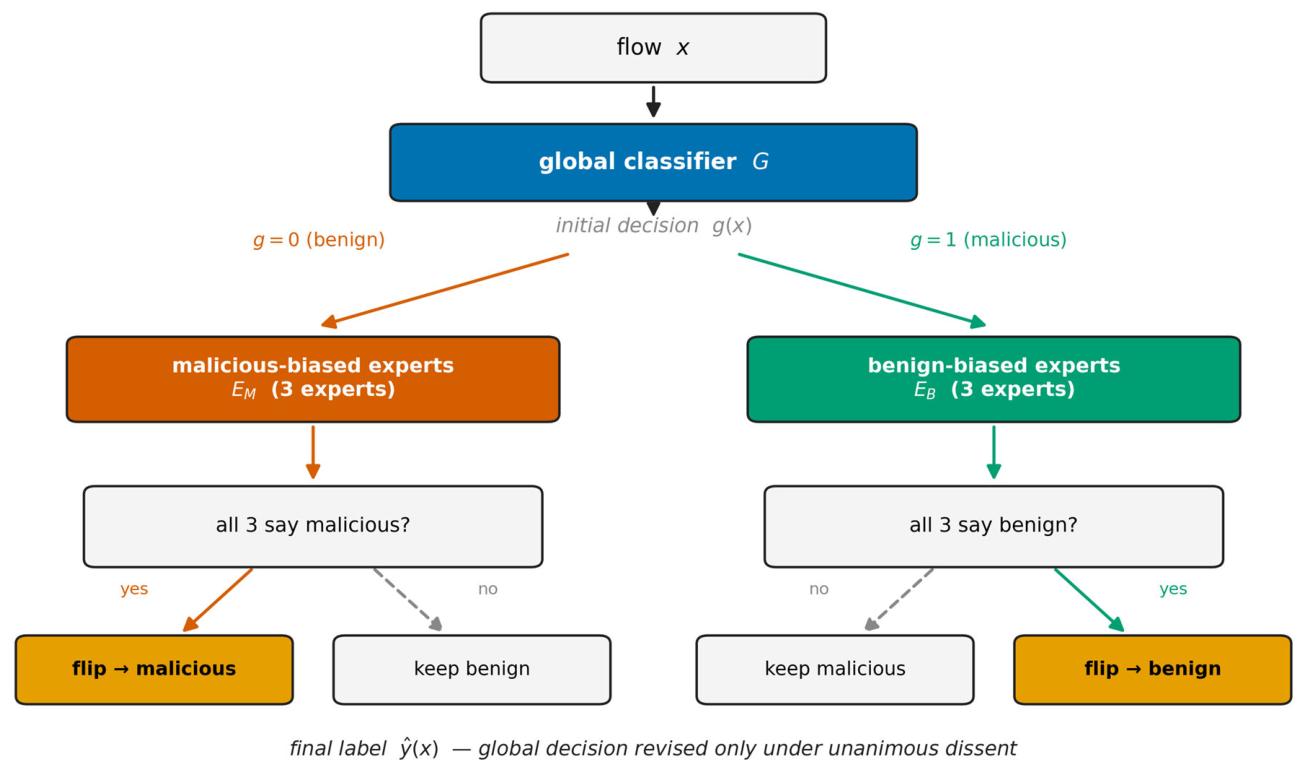
This is the direction taken by conditional counter-inspection with curriculum-biased experts [1]. The original architecture used a homogeneous CART implementation: one global decision tree and two groups of class-biased decision tree experts. An initially benign prediction was inspected only by malicious-biased experts and an initially malicious prediction only by benign-biased experts, and the initial label was revised only when every expert in the activated branch unanimously provided counter-evidence. Evaluated on 5G-NIDD, the method reduced the errors of the standalone decision tree while preserving a lightweight, deterministic inference structure [1].

That homogeneous design, however, left four questions open. First, because every component was a CART tree, it was unclear whether missed-attack recovery arose from the conditional architecture or from the specific behavior of decision trees. Second, the design did not establish whether changing the learner in each expert branch could control the balance between false positives and false negatives. Third, the system was reported through one principal configuration, leaving unexamined whether the architecture could supply different operating profiles for different deployment priorities. Fourth, its global classifier was already strong, so it remained unknown whether counter-inspection could recover useful performance from a weaker first-stage detector.

These questions cannot be settled by replacing the global model with a uniformly stronger one. A stronger global learner may lower total error, but it does not reveal how the functional roles interact, because the global classifier and the two expert branches receive different training distributions and intervene at different points in the decision process. Assigning one algorithm to all three roles imposes a homogeneity constraint that the routing mechanism does not require. Removing it allows for learner diversity to be studied while the curriculum construction, conditional activation, and unanimous dissent rule are held fixed.

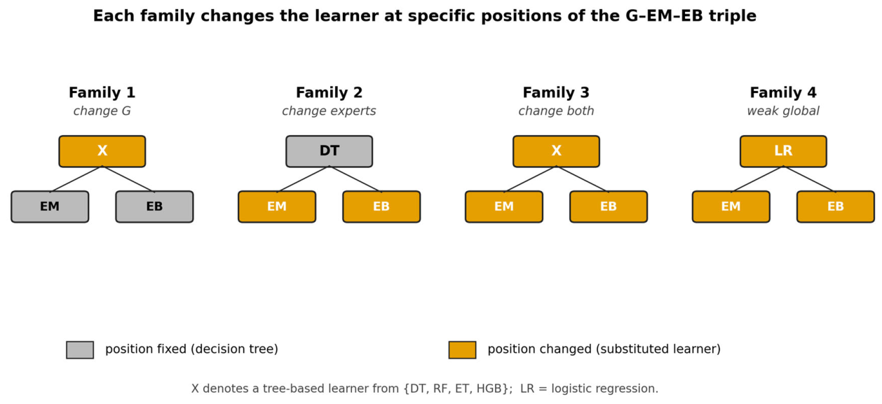
This study generalizes the pipeline into a heterogeneous configuration denoted G–EM–EB, where G is the global classifier, EM the malicious-biased expert backbone, and EB the benign-biased expert backbone. Decision tree (DT), random forest (RF), extremely randomized trees (ET), and histogram-based gradient boosting (HGB) are assigned to these roles through controlled homogeneous and heterogeneous substitutions, and logistic regression (LR) is used additionally as a deliberately weaker global filter. The evaluation uses two datasets of contrasting difficulty: 5G-NIDD, labeled benign and attack traffic collected over a functional 5G test network, which places several tree-based classifiers in a near-ceiling regime [7], and UNSW-NB15, a harder general benchmark used to test whether the observed behavior persists when the first-stage models leave substantially more residual error [8].

As a concrete deployment scenario, consider an intrusion detector running at the network edge or on a multi-access edge computing (MEC) node in a softwarized 5G network, where flow-level features are already collected for monitoring. A first-stage classifier issues an initial decision, and the conditional validation layer re-examines only the uncertain class before an alert is raised or suppressed. In such a setting, the operator must balance missed attacks against false alarms under tight latency and memory budgets, which is precisely the balance the configurable architecture studied here is designed to control. This scenario motivates the contributions that follow.

The aim is not to identify a universally superior learner, but to determine whether the conditional architecture preserves its security function across learner substitutions and whether different assignments expose controllable error profiles. The contributions of this work are as follows:

• Missed-attack recovery across tree-based learners. We show that the security function of conditional counter-inspection, recovering attacks missed by the first stage, is not specific to decision trees. Across both datasets, all fourteen evaluated tree-based configurations reduce false negatives, establishing the effect as a property of the conditional architecture rather than of any single learner.
• Expert-driven error control. By fixing the global classifier and varying only the expert backbone, we demonstrate that the expert choice selects which error the system controls, shifting the balance between false positives and false negatives within a fixed decision mechanism rather than improving both uniformly.
• Deployment-oriented operating profiles. We characterize heterogeneous G–EM–EB assignments as distinct operating points for aggregate F1, attack recovery, and false-alarm control, reported as observed profiles rather than validation-selected optima, so that model selection can follow a deployment’s relative cost of missed attacks and false alarms.
• Weak-filter recovery. We show that tree-based counter-inspection can restore competitive detection from a deliberately weak logistic regression first stage, yielding the largest absolute F1 gain observed in the study on UNSW-NB15, without retraining or replacing the deployed classifier.
• Measured efficiency. We quantify inference cost on both datasets, confirming that the pipeline evaluates at most four of its seven models per record and keeps classifier inference below 0.1 ms per record, so the configurability is obtained at a modest and bounded computational cost.

In relation to our previous work, the novelty of this study is explicit. Paper 1 [1] introduced conditional counter-inspection as a homogeneous CART pipeline and reported it as a single fixed configuration, leaving open whether its benefits came from the conditional architecture or from decision trees. The present work does not re-tune or incrementally improve that pipeline; it investigates whether the architecture can act as a configurable, heterogeneous validation layer. Concretely, and unlike Paper 1, we (i) decouple the three functional roles so that different learners can occupy the global and expert positions, (ii) show that the expert assignment deliberately selects the error the system controls, (iii) expose distinct deployment-oriented operating profiles from one architecture, and (iv) demonstrate weak-filter recovery of a non-tree global classifier. The focus thus shifts from improving a single CART detector to selecting expert assignments that yield different operational profiles: missed-attack recovery, false-alarm suppression, best F1 operation, or weak-filter recovery.

Collectively, these contributions reframe conditional counter-inspection from a fixed, homogeneous detector into a configurable validation architecture: a single deterministic structure of bounded inference cost whose error profile is determined by the learner assigned to each functional role, and which can be matched to the operational cost structure of a given deployment rather than optimized for one aggregate metric.

All experiments use controlled preprocessing and fixed data partitions, and each pipeline is compared with an appropriate reference: its standalone global classifier, the homogeneous DT–DT–DT architecture, or standalone logistic regression. Alongside accuracy, precision, recall, and F1, raw false positive and false negative counts are retained because they expose operational changes that aggregate metrics can hide.

The remainder of the paper is organized as follows: Section 2 formalizes the heterogeneous architecture, the curriculum-biased expert construction, the conditional decision rule, and the experimental protocol. Section 3 reports the results on missed-attack recovery, expert-driven error control, deployment-oriented profiles, weak-filter recovery, and controlled positioning against the homogeneous CART reference. The Section 4 discusses implications, limitations, and directions for future work.

2. Methodology

2.1. Scope

The conditional counter-inspection pipeline used in this work was introduced in our previous study [1], where its full design, curriculum construction, and homogeneous decision tree implementation are described. We do not restate that development. This section gives a short reminder of how the pipeline makes a prediction (Section 2.2) and then defines the single change studied here: using learners other than the decision tree at chosen positions of the pipeline, while leaving the routing and decision rule exactly as in [1].

2.2. How the Pipeline Makes a Prediction

A flow is classified in two stages (Figure 1). A global classifier $G$ makes an initial benign-or-malicious decision. A small group of class-biased experts then re-examines that decision and can overturn it, but only by unanimous disagreement. Concretely, for a flow $x$:

• The global classifier predicts an initial label $g\left(x\right)=G\left(x\right)\in \{0,1\}$, where $1$ denotes the malicious (positive) class.
• Only the experts for the opposite class are consulted: if $g\left(x\right)=0$, the malicious-biased experts $E_M$ inspect the flow; if $g\left(x\right)=1$, the benign-biased experts $E_B$ inspect it. The same-class experts are never evaluated.
• The label is flipped only if every consulted expert disagrees with $G$ ; any single agreeing expert leaves the decision unchanged.

Each branch holds three experts, trained at the opposite-class exposure fractions $\rho \in R=\{0.10,0.20,0.30\}$ [1]. Writing the two unanimity indicators over these experts as

$$u_M\left(x\right)=\prod _{\rho \in R}{E}_M^{\left(\rho \right)}\left(x\right), u_B\left(x\right)=\prod _{\rho \in R}\left[\hspace{0.17em}1-E_B^{\left(\rho \right)}\left(x\right)\hspace{0.17em}\right],$$

and noting that expert outputs are binary, $u_M\left(x\right)=1$ exactly when all three malicious-biased experts predict malicious, and $u_B\left(x\right)=1$ exactly when all three benign-biased experts predict benign. The final decision is

$$\widehat{y}\left(x\right)=\left[\hspace{0.17em}1-g\left(x\right)\hspace{0.17em}\right]\hspace{0.17em}{u}_M\left(x\right)\hspace{0.33em}+\hspace{0.33em}g\left(x\right)\hspace{0.17em}\left[\hspace{0.17em}1-u_B\left(x\right)\hspace{0.17em}\right],$$

which flips an initial benign decision to malicious only when $u_M\left(x\right)=1$, flips an initial malicious decision to benign only when $u_B\left(x\right)=1$, and otherwise returns $g\left(x\right)$. A pipeline therefore holds seven models in total, one global and two branches of three, but evaluates at most four per flow, since only one branch is consulted; the correction is deterministic and needs no threshold tuning.

2.3. The Single Change Studied and the Experimental Families

A configuration is written in the order G–EM–EB, where $G$ is the learner at the global classifier, $\mathrm{E}\mathrm{M}$ the learner in the malicious-biased branch, and $\mathrm{E}\mathrm{B}$ the learner in the benign-biased branch; in this notation the original pipeline of [1] is the homogeneous case DT–DT–DT. The present study keeps this pipeline identical and asks one question: what happens when a different learner is placed at one or more of the three positions? Swapping a learner changes only how that position is trained and votes (never the routing, the number of experts, or the unanimous dissent rule), so any change in results is attributable to learner placement rather than to the decision logic. Formally, a configuration is the triple $\mathcal{C}=\left(a_G,a_M,a_B\right)$, with the biased expert sets built for each $\rho \in R$ as ${\mathcal{D}}_M^{\left(\rho \right)}={\mathcal{D}}_M\cup S_{\rho }\left({\mathcal{D}}_B\right)$ and ${\mathcal{D}}_B^{\left(\rho \right)}={\mathcal{D}}_B\cup S_{\rho }\left({\mathcal{D}}_M\right)$, so each malicious-biased expert sees every malicious flow and only a fraction $\rho$ of benign flows, and symmetrically for the benign-biased experts.

Four tree-based learners form the substitution set:

$${\mathcal{A}}_T=\{\mathrm{D}\mathrm{T},\mathrm{R}\mathrm{F},\mathrm{E}\mathrm{T},\mathrm{H}\mathrm{G}\mathrm{B}\},$$

spanning single-tree (DT [9]), bagging (RF [10], ET [11]), and boosting (HGB [12]) behavior while remaining practical for flow-level detection; logistic regression (LR [13]) is reserved for the global position as a deliberately weak first stage. No per-configuration tuning is performed: each learner uses one fixed implementation and seed wherever it appears.

The experiments are organized not by the many individual configurations but by the simple question of which positions are changed (Figure 2). Concretely, the global classifier may be changed while the experts are held fixed, $X–\mathrm{D}\mathrm{T}–\mathrm{D}\mathrm{T}$ with $X\in {\mathcal{A}}_T$; the experts may be changed while the global is held fixed as a decision tree, $\mathrm{D}\mathrm{T}–X–X$; both may be changed together, either homogeneously, $X–X–X$, or asymmetrically, $X–Y–Z$ with $X,Y,Z\in {\mathcal{A}}_T$; and the global may be set to a weak linear filter with tree-based experts, $\mathrm{L}\mathrm{R}–Y–Z$. The asymmetric case is not an exhaustive search over the $4^3=64$ possible tree-based triples but a targeted set chosen to expose deployment-oriented behavior: aggregate F1 improvement, DT-compatible recovery, single-branch replacement, and aggressive missed-attack recovery.

Table 1. The experimental families, organized by which position of the G–EM–EB triple is changed. DT, RF, ET, and HGB are tree-based learners (${\mathcal{A}}_T$); LR is logistic regression. The first stage is the global classifier; the validation layer is the two expert branches.

Position Changed	Configuration Form	Question Addressed
Global classifier only	X–DT–DT, X ∈ A_T	Does missed-attack recovery survive replacing the first stage?
Experts only	DT–X–X, X ∈ A_T	Does the validation layer control the FP/FN balance?
Both (homogeneous and asymmetric)	X–X–X and X–Y–Z	Does the effect persist beyond DT, and can distinct operating profiles be exposed?
Global set to a weak learner	LR–Y–Z, Y, Z ∈ A_T	Can the experts recover a deliberately weak first stage?

summarizes these families by the position they vary and the question each addresses.

Configuration Selection Rationale

The heterogeneous configurations were not selected by an arbitrary or brute-force sweep of the 64 possible tree-based triples. The exploration is structured around functional roles, so that each family answers a specific question rather than contributing to a leaderboard: (i) the global classifier is varied with the experts fixed as decision trees (X–DT–DT), isolating the first stage; (ii) the experts are varied with the global fixed as a decision tree (DT–X–X), isolating the validation layer; (iii) homogeneous replacements (X–X–X) test whether the effect is specific to CART; (iv) a small number of asymmetric configurations are then examined, guided by the branch-level behavior observed in (i)–(ii), to represent distinct operating profiles: best aggregate F1, DT-compatible recovery, single-branch modification, and aggressive missed-attack recovery; and (v) logistic regression is used only as a weak-global stress test. The aim is controlled role analysis, not exhaustive optimization: a full 64-configuration sweep would identify a numerically best triple but would not explain how the functional roles shape the error profile, which is the question this study addresses. The complete set of evaluated configurations is reported in Appendix A.

2.4. Datasets and Preprocessing

Two public benchmarks of contrasting difficulty are used. 5G-NIDD, collected from a functional 5G test network [7], is a near-ceiling regime where tree-based classifiers already perform very well. UNSW-NB15 [8] is a harder general benchmark that leaves more residual error. Malicious traffic is the positive class; a false positive (FP) is a benign flow predicted malicious, and a false negative (FN) a malicious flow predicted benign.

For 5G-NIDD, the target is mapped to 0/1, categorical fields are one-hot encoded with an explicit unknown category, and the same stratified 80/20 split as in [1] yields 972,712 training and 243,178 test records (malicious prevalence 0.607 in both). For UNSW-NB15, the predefined partitions are kept: 82,332 training and 175,341 test records of 45 attributes, the distributed test set being the larger and preserved unchanged for comparability, and one-hot encoding giving 190 features (malicious prevalence 0.5506 train, 0.6806 test). For both datasets, all transformations are fitted only on training data and applied unchanged to test data, and every configuration on a dataset uses identical processed instances, so differences come from learner placement rather than preprocessing.

2.5. Evaluation and Reproducibility

Results are reported with accuracy, precision, recall, and F1 (malicious as positive), alongside raw FP and FN counts, which expose operational changes that aggregate metrics hide. With TP, TN, FP, and FN the usual confusion-matrix counts are

$$\mathrm{A}\mathrm{c}\mathrm{c}\mathrm{u}\mathrm{r}\mathrm{a}\mathrm{c}\mathrm{y}={\displaystyle \frac{TP+TN}{TP+TN+FP+FN}},$$

$$\mathrm{P}\mathrm{r}\mathrm{e}\mathrm{c}\mathrm{i}\mathrm{s}\mathrm{i}\mathrm{o}\mathrm{n}={\displaystyle \frac{TP}{TP+FP}},$$

$$\mathrm{R}\mathrm{e}\mathrm{c}\mathrm{a}\mathrm{l}\mathrm{l}={\displaystyle \frac{TP}{TP+FN}},$$

$$F_1={\displaystyle \frac{2\hspace{0.17em}\mathrm{P}\mathrm{r}\mathrm{e}\mathrm{c}\mathrm{i}\mathrm{s}\mathrm{i}\mathrm{o}\mathrm{n}\cdot \mathrm{R}\mathrm{e}\mathrm{c}\mathrm{a}\mathrm{l}\mathrm{l}}{\mathrm{P}\mathrm{r}\mathrm{e}\mathrm{c}\mathrm{i}\mathrm{s}\mathrm{i}\mathrm{o}\mathrm{n}+\mathrm{R}\mathrm{e}\mathrm{c}\mathrm{a}\mathrm{l}\mathrm{l}}}.$$

For an error count $q\in \{FP,FN\}$, the signed relative change against a reference is $\mathsf{\Delta }q\left(\mathrm{\%}\right)=100\hspace{0.17em}\left(q_{\mathrm{p}\mathrm{i}\mathrm{p}\mathrm{e}\mathrm{l}\mathrm{i}\mathrm{n}\mathrm{e}}-q_{\mathrm{r}\mathrm{e}\mathrm{f}\mathrm{e}\mathrm{r}\mathrm{e}\mathrm{n}\mathrm{c}\mathrm{e}}\right)/q_{\mathrm{r}\mathrm{e}\mathrm{f}\mathrm{e}\mathrm{r}\mathrm{e}\mathrm{n}\mathrm{c}\mathrm{e}}$, so negative values denote reductions; F1 differences are reported as absolute changes. References differ by experiment: substitution and expert families use the matching standalone global classifier, deployment profiles use the homogeneous DT–DT–DT pipeline, and weak-filter recovery uses standalone logistic regression. The profiles highlighted in Section 3.3 are observed on the held-out test set, not selected on a separate validation set.

For reproducibility, the curriculum subsets are sampled once with fixed seeds and reused across all substitutions, so configurations with different learners see identical role-specific training data. No test record is used for encoding, subset construction, training, or configuration selection; the held-out test partition is used only for final inference and the comparisons reported in Section 3. The implementation uses Python and scikit-learn [13]; exact versions, the random seed, and any non-default parameters accompany the final manuscript.

To support full reproducibility, the exact software environment and learner settings are specified here. All experiments were implemented in Python 3.12.13 (Python Software Foundation, Wilmington, DE, USA), using scikit-learn 1.6.1, NumPy 2.0.2, pandas 2.2.2, and SciPy 1.16.3, all open-source scientific-computing libraries maintained under the NumFOCUS umbrella (Austin, TX, USA), executed under a single fixed random seed (42) governing all data sampling and stochastic learners. The learner settings are those listed in

Table 2. Learner configurations and reproducibility settings. All stochastic components use random seed 42; unlisted parameters use scikit-learn defaults.

Component	Learner/Setting	Key Hyperparameters
Global/experts: DT	DecisionTreeClassifier	defaults, random_state = 42
Global/experts: RF	RandomForestClassifier	n_estimators = 200, random_state = 42; n_jobs = −1 for training, n_jobs = 1 for timing
Global/experts: ET	ExtraTreesClassifier	n_estimators = 200, random_state = 42; n_jobs = −1 for training, n_jobs = 1 for timing
Global/experts: HGB	HistGradientBoostingClassifier	defaults, random_state = 42
Weak global: LR	median impute → StandardScaler → LogisticRegression	max_iter = 3000, solver = ‘lbfgs’
Curriculum fractions	opposite-class exposure	{0.10, 0.20, 0.30}; 3 EM + 3 EB experts
Split: 5G-NIDD	stratified train/test	80/20, random_state = 42
Split: UNSW-NB15	predefined partitions	82,332 train/175,341 test
Environment	Python/libraries	Python 3.12, scikit-learn 1.6.1, NumPy 2.0.2, pandas 2.2.2, SciPy 1.16.3

: default scikit-learn hyperparameters are used except where noted, with no per-configuration tuning, so that performance differences reflect learner placement rather than unequal optimization. The 5G-NIDD auxiliary columns Attack Type and Attack Tool are removed prior to training to prevent label leakage; encoders and biased subsets are fitted on the training data only. The trained models, derived-result tables, and full implementation are available from the corresponding author on reasonable request.

3. Results

This section evaluates four operational properties of the enhanced conditional counter-inspection pipeline on two datasets with different levels of difficulty. On 5G-NIDD, the standalone tree-based classifiers already operate near ceiling, whereas UNSW-NB15 leaves substantially more residual error. This contrast allows for the architecture to be examined both as a fine-grained corrective layer and under a more challenging detection regime.

Malicious traffic is treated as the positive class. Accordingly, a false positive (FP) is a benign flow incorrectly classified as malicious, whereas a false negative (FN) is a malicious flow incorrectly classified as benign. Each pipeline configuration is denoted in the order G–EM–EB, where G is the first-stage global classifier, EM is the malicious-biased validation branch activated after an initial benign prediction, and EB is the benign-biased validation branch activated after an initial malicious prediction. DT, RF, ET, HGB, and LR denote decision tree, random forest, extremely randomized trees, histogram-based gradient boosting, and logistic regression, respectively.

The reference used depends on the purpose of each analysis. In Section 3.1 and Section 3.2, each pipeline is compared with its corresponding standalone global classifier. Section 3.3 uses the homogeneous DT–DT–DT pipeline as the architectural reference, while Section 3.4 evaluates improvement relative to standalone LR. Unless otherwise stated, negative changes in FP or FN denote reductions in the corresponding error type, whereas positive changes denote increases. Differences in F1 are reported as absolute values throughout.

3.1. Missed-Attack Recovery

The first question is whether the missed-attack recovery observed in the original homogeneous CART implementation [1] depends on that specific learner. To examine this, the DT-based components are replaced by alternative tree-based learners using two substitution patterns: global-only substitution with DT experts and homogeneous substitution using the same learner at all three levels. Together with the original DT–DT–DT pipeline, this produces seven evaluated configurations per dataset.

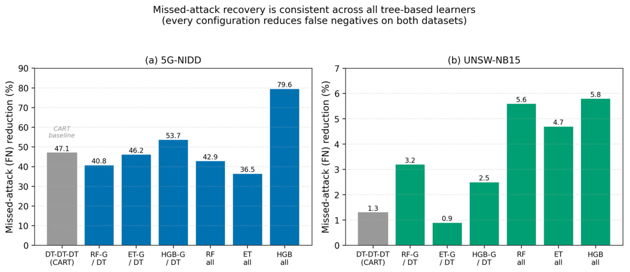
The recovery effect is consistent across this evaluated set. Every configuration reduces false negatives relative to its corresponding standalone global classifier, yielding fourteen reductions across fourteen dataset configuration cases. On 5G-NIDD, the reductions range from 36.5% to 79.6%. The strongest result is obtained with HGB–HGB–HGB, which reduces missed attacks from 54 to 11. The original DT–DT–DT pipeline achieves a 47.1% reduction and lies within the range of the alternative configurations rather than at its upper limit.

The same direction is observed on UNSW-NB15. Although the relative reductions are smaller, ranging from 0.9% to 5.8%, all seven configurations again recover part of the attack traffic missed by the first-stage classifier. The strongest relative reduction is obtained with HGB–HGB–HGB, which lowers FN from 16,657 to 15,697. Figure 3 shows the per-configuration reductions on both datasets.

The effect on aggregate F1 is more selective. F1 improves in five of the seven configurations on 5G-NIDD and four of the seven configurations on UNSW-NB15. Improvement is more likely when the global classifier leaves enough residual error for the validation branches to correct. When the global classifier already operates near ceiling, as with HGB on 5G-NIDD, recovering additional attacks may be accompanied by enough new false positives to slightly reduce aggregate F1.

These results establish that missed-attack recovery is not specific to the original CART-only implementation. Across the evaluated global-only and homogeneous substitutions involving DT, RF, ET, and HGB, conditional counter-inspection consistently reduces the attacks missed by the first stage. Complete configuration-level results are reported in Appendix A (

Table A1. Complete configuration-level results for the tree-based substitution experiment (Section 3.1). Values are standalone global → pipeline. ΔFP and ΔFN are signed counts (negative = reduction); FN reduction (%) is a positive magnitude. Rows with DT experts vary only the global classifier; rows with matched G/EM/EB use a single backbone at all levels.

Dataset	Configuration (G–EM–EB)	F1 (Global → Pipeline)	ΔF1	FP (Global → Pipeline)	ΔFP	FN (Global → Pipeline)	ΔFN	FN Reduction (%)
5G-NIDD	DT–DT–DT (CART baseline)	0.999665 → 0.999807	+0.000142	48 → 30	−18	51 → 27	−24	47.1%
5G-NIDD	RF–DT–DT	0.999675 → 0.999800	+0.000125	47 → 30	−17	49 → 29	−20	40.8%
5G-NIDD	ET–DT–DT	0.999662 → 0.999804	+0.000142	48 → 30	−18	52 → 28	−24	46.2%
5G-NIDD	HGB–DT–DT	0.999807 → 0.999719	−0.000088	3 → 58	+55	54 → 25	−29	53.7%
5G-NIDD	RF–RF–RF	0.999675 → 0.999810	+0.000135	47 → 28	−19	49 → 28	−21	42.9%
5G-NIDD	ET–ET–ET	0.999661 → 0.999736	+0.000075	48 → 45	−3	52 → 33	−19	36.5%
5G-NIDD	HGB–HGB–HGB	0.999807 → 0.999594	−0.000213	3 → 109	+106	54 → 11	−43	79.6%
UNSW-NB15	DT–DT–DT (CART baseline)	0.915221 → 0.918558	+0.003337	2074 → 1515	−559	16,904 → 16,688	−216	1.3%
UNSW-NB15	RF–DT–DT	0.925225 → 0.922108	−0.003117	1287 → 1432	+145	16,548 → 16,023	−525	3.2%
UNSW-NB15	ET–DT–DT	0.922089 → 0.922044	−0.000045	1239 → 1417	+178	16,192 → 16,049	−143	0.9%
UNSW-NB15	HGB–DT–DT	0.920149 → 0.920862	+0.000713	785 → 1475	+690	16,657 → 16,245	−412	2.5%
UNSW-NB15	RF–RF–RF	0.925224 → 0.925719	+0.000495	1287 → 2180	+893	15,498 → 14,625	−873	5.6%
UNSW-NB15	ET–ET–ET	0.922088 → 0.921372	−0.000716	1239 → 2305	+1066	16,192 → 15,430	−762	4.7%
UNSW-NB15	HGB–HGB–HGB	0.920149 → 0.922736	+0.002587	785 → 1660	+875	16,657 → 15,697	−960	5.8%

).

3.2. Expert-Driven Error Control

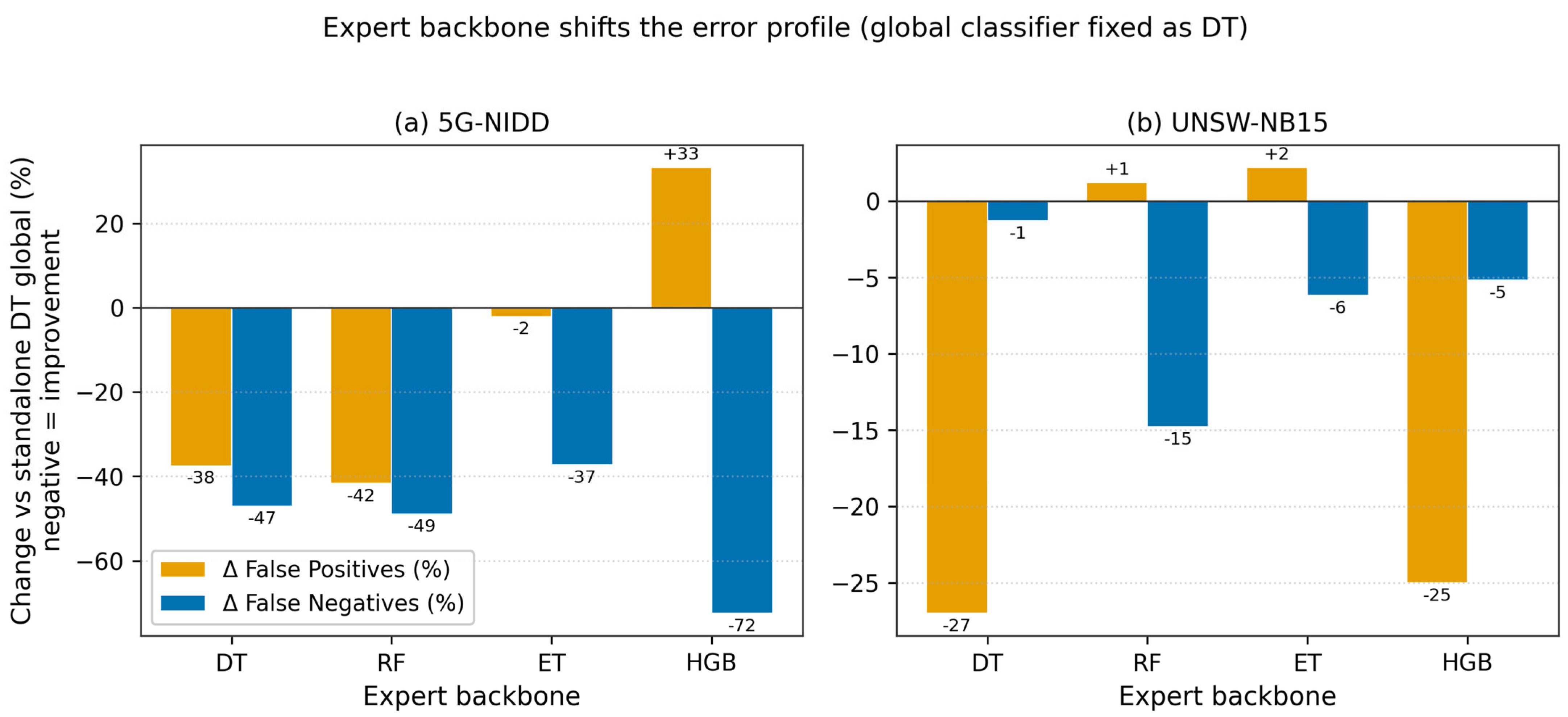
If expert substitution only changed the overall strength of the validation layer, false positives and false negatives might be expected to move in the same direction. The results instead show that the expert backbone changes the balance between the two error types. To isolate this effect, the global classifier is fixed as DT while the same learner is assigned to both expert branches, producing DT–X–X configurations with X ∈ {DT, RF, ET, HGB}.

The clearest contrast appears on 5G-NIDD. With RF experts, false positives fall from 48 to 28, corresponding to a 41.7% reduction, while false negatives decrease from 51 to 26, corresponding to a 49.0% reduction. This is the most balanced profile among the evaluated expert backbones on this dataset. HGB experts produce a different operating profile: FN decreases from 51 to 14, a 72.5% reduction, while FP increases from 48 to 64. Changing only the expert backbone can therefore shift the same DT first-stage detector from balanced correction toward more aggressive missed-attack recovery.

The profiles also vary across datasets. On UNSW-NB15, HGB experts reduce FP by 25.0% and FN by 5.2%, producing a predominantly false-alarm-oriented correction. RF experts obtain the highest F1 among the DT-global expert variants, reducing FN by 14.8% while increasing FP by only 24 instances. The different behavior of the same expert family across datasets indicates that the resulting error profile depends on the residual errors presented to the validation branches, rather than on a fixed ranking of learners.

Table 3. Expert backbone effect with the global classifier fixed as DT. The selected backbone is assigned to both EM and EB. FP and FN changes are calculated relative to the standalone DT global classifier. Negative values denote reductions, while positive values denote increases.

Dataset	Expert Backbone	FP Change	FN Change	F1	Observed Profile
5G-NIDD	DT	−37.5%	−47.1%	0.999807	Homogeneous CART reference
5G-NIDD	RF	−41.7%	−49.0%	0.999817	Balanced error reduction
5G-NIDD	ET	−2.1%	−37.3%	0.999732	Recall-oriented correction
5G-NIDD	HGB	+33.3%	−72.5%	0.999736	Aggressive FN reduction
UNSW-NB15	DT	−27.0%	−1.3%	0.918558	Predominantly FP reduction
UNSW-NB15	RF	+1.2%	−14.8%	0.927151	Highest F1 among DT-global variants
UNSW-NB15	ET	+2.2%	−6.2%	0.920116	Moderate FN reduction
UNSW-NB15	HGB	−25.0%	−5.2%	0.921549	Joint reduction, mainly FP-oriented

reports the full expert backbone comparison for both datasets, and Figure 4 visualizes the resulting error profiles as percentage changes in FP and FN.

The expert layer therefore does not act as a uniform performance booster. Its composition changes the direction and magnitude of the correction, making the balance between missed attacks and false alarms adjustable within the same conditional architecture.

3.3. Deployment-Oriented Operating Profiles

The profiles identified in Section 3.2 are operationally relevant because intrusion detection deployments rarely assign the same cost to false positives and false negatives. Missed attacks may dominate the cost in high-security environments, whereas excessive false alarms may be more disruptive in high-volume monitoring systems.

To make the comparison reproducible and avoid treating every selected configuration as an unconditional optimum, three explicit profile criteria are used: (1) best aggregate performance, corresponding to the highest F1 over the evaluated tree-based configuration space; (2) DT-compatible recovery, represented by a configuration that retains DT as the first-stage classifier while providing a substantial reduction in false negatives; and (3) single-branch FP control, a minimal-modification profile obtained by retaining the DT global and DT malicious validation branch while replacing only the benign validation branch. These criteria distinguish an overall performance optimum from configurations selected under compatibility or modification constraints. The configurations highlighted under each criterion are observed operating profiles identified from the evaluated results on the held-out test set; they are reported as illustrative operating points rather than independently validation-selected optima. The complete heterogeneous configuration results are provided in Appendix A (

Table A2. Heterogeneous (hybrid) configuration results supporting Section 3.3. Configuration order is G–EM–EB. Values are pipeline counts on the held-out test set; ΔFP, ΔFN (percentages) and ΔF1 (absolute) are relative to the homogeneous DT–DT–DT reference on the same dataset.

Dataset	Configuration	FP	FN	F1	ΔFP	ΔFN	ΔF1
5G-NIDD	DT–RF–HGB	13	30	0.999854	−56.7%	+11.1%	+0.000047
5G-NIDD	DT–HGB–RF	79	10	0.999699	+163.3%	−63.0%	−0.000108
5G-NIDD	DT–DT–HGB	15	31	0.999844	−50.0%	+14.8%	+0.000037
5G-NIDD	DT–RF–RF	28	26	0.999817	−6.7%	−3.7%	+0.000010
5G-NIDD	RF–RF–HGB	13	32	0.999848	−56.7%	+18.5%	+0.000041
5G-NIDD	HGB–HGB–RF	109	8	0.999604	+263.3%	−70.4%	−0.000203
UNSW-NB15	HGB–RF–RF	2356	13,893	0.928464	+55.5%	−16.7%	+0.009906
UNSW-NB15	DT–RF–RF	2098	14,394	0.927151	+38.5%	−13.7%	+0.008593
UNSW-NB15	DT–RF–HGB	2218	14,338	0.926925	+46.4%	−14.1%	+0.008367
UNSW-NB15	DT–HGB–RF	1436	16,089	0.921774	−5.2%	−3.6%	+0.003216
UNSW-NB15	DT–DT–HGB	1241	18,322	0.911720	−18.1%	+9.8%	−0.006838
UNSW-NB15	HGB–HGB–RF	1524	16,387	0.919976	+0.6%	−1.8%	+0.001418

). The resulting profiles are summarized in

Table 4. Representative deployment-oriented profiles. Configuration order is G–EM–EB. Changes are calculated relative to the homogeneous DT–DT–DT reference on the same dataset. Negative ΔFP and ΔFN values denote error reductions; ΔF1 is an absolute difference.

Dataset	Profile Criterion	Configuration	FP	FN	F1	ΔFP	ΔFN	ΔF1
5G-NIDD	Homogeneous reference	DT–DT–DT	30	27	0.999807	—	—	—
5G-NIDD	Best aggregate performance	DT–RF–HGB	13	30	0.999854	−56.7%	+11.1%	+0.000047
5G-NIDD	DT-compatible recovery	DT–HGB–RF	79	10	0.999699	+163.3%	−63.0%	−0.000108
5G-NIDD	Single-branch FP control	DT–DT–HGB	15	31	0.999844	−50.0%	+14.8%	+0.000037
UNSW-NB15	Homogeneous reference	DT–DT–DT	1515	16,688	0.918558	—	—	—
UNSW-NB15	Best aggregate performance	HGB–RF–RF	2356	13,893	0.928464	+55.5%	−16.7%	+0.009906
UNSW-NB15	DT-compatible recovery	DT–RF–RF	2098	14,394	0.927151	+38.5%	−13.7%	+0.008593
UNSW-NB15	Single-branch FP control	DT–DT–HGB	1241	18,322	0.911720	−18.1%	+9.8%	−0.006838

.

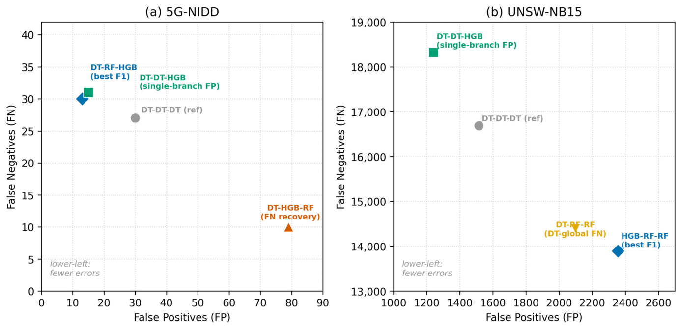
On 5G-NIDD, the best F1 configuration, DT–RF–HGB, reaches an F1 of 0.999854 and reduces FP from 30 to 13 relative to the homogeneous DT–DT–DT pipeline. Its FN count increases slightly from 27 to 30, showing that the F1 gain is primarily driven by false-alarm reduction. The DT-compatible recovery profile, DT–HGB–RF, reduces FN from 27 to 10 but increases FP from 30 to 79. It therefore represents a security-oriented operating point rather than a general performance optimum.

The DT–DT–HGB configuration illustrates a lower-disruption adjustment. By changing only EB, FP is reduced from 30 to 15 while the global classifier and malicious validation branch remain unchanged. This profile is not presented as the overall minimum-FP solution, because it is dominated in raw FP and FN counts by DT–RF–HGB. Its value lies in showing that a substantial reduction in false alarms can be obtained through a single expert-branch replacement.

On UNSW-NB15, the highest F1 among the evaluated tree-based configurations is achieved by HGB–RF–RF, which raises F1 from 0.918558 to 0.928464 and reduces FN by 16.7%, while increasing FP by 55.5%. When retaining DT as the global classifier, DT–RF–RF provides a compatible recovery profile, reducing FN by 13.7% and increasing F1 by 0.008593. The single-branch DT–DT–HGB profile reduces FP by 18.1% but increases FN by 9.8% and lowers F1. It is therefore appropriate only when reducing alert volume has a higher operational priority than missed-attack recovery.

Figure 5 maps these profiles in the FP–FN plane. The homogeneous reference provides a common origin for interpreting movement toward lower false-alarm counts or lower missed-attack counts. The figure does not imply that every labeled point is Pareto-optimal; rather, it distinguishes the overall best F1 configuration from profiles selected under first-stage compatibility or minimal-modification constraints.

The pipeline does not eliminate the trade-off between missed attacks and false alarms. Its contribution is to expose that trade-off through identifiable configurations, allowing for model selection to reflect the operational cost structure of the deployment.

3.4. Weak-Filter Recovery

A practical IDS does not always begin with a strong first-stage classifier. Legacy detectors, lightweight filters, or simple linear models may remain in use because they are fast, available, or already integrated into an operational system. A useful corrective architecture should therefore be able to recover performance from a weak first-stage filter rather than requiring its immediate replacement.

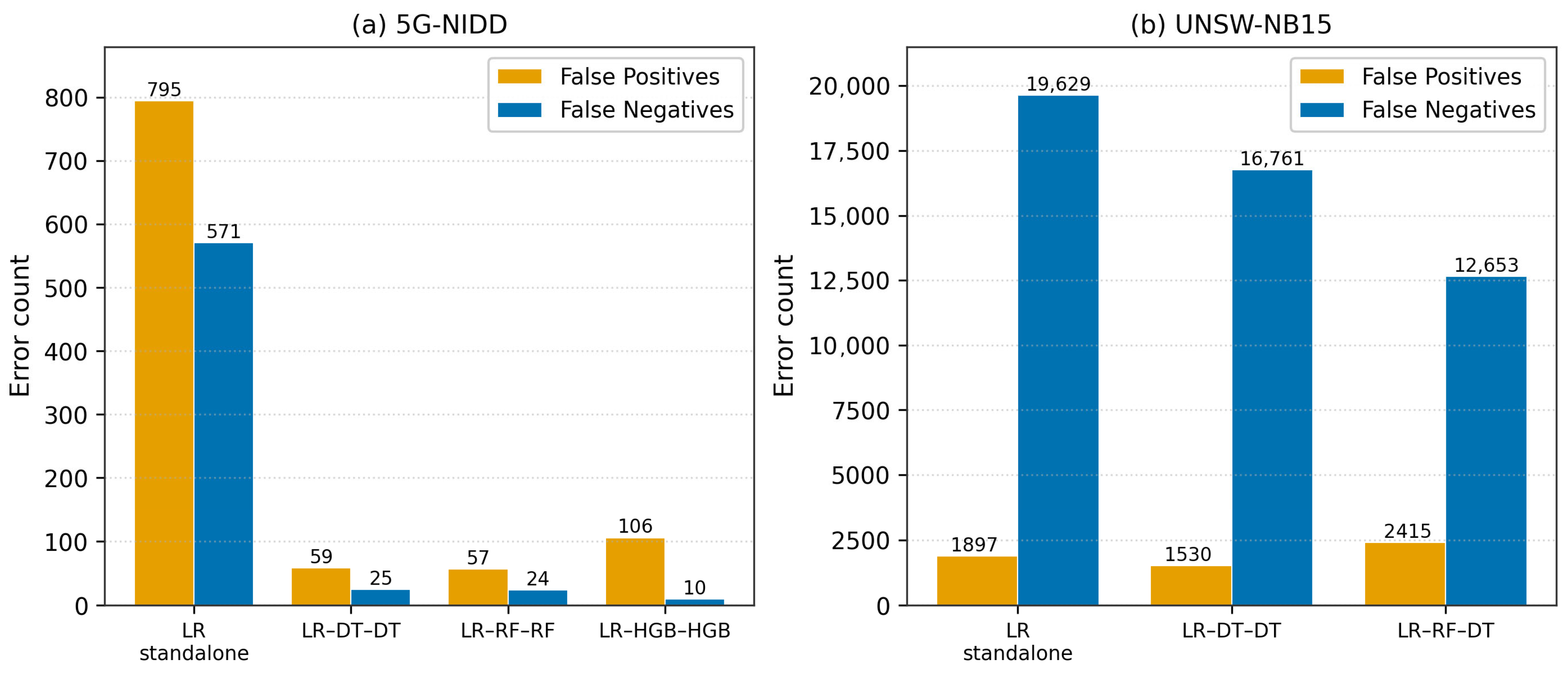
To examine this property, LR is used as the global classifier and paired with tree-based validation experts. On 5G-NIDD, standalone LR produces 795 FP and 571 FN. With RF assigned to both expert branches, these counts fall to 57 and 24, corresponding to reductions of 92.8% and 95.8%, respectively. F1 increases from 0.994410 to 0.999726. HGB experts provide the strongest attack recovery, reducing FN to 10, although their FP count is higher than that obtained with DT or RF experts. The complete weak-filter grid is reported in Appendix A (

Table A3. Complete weak-filter (LR global) configuration results supporting Section 3.4. Configuration order is G–EM–EB. ΔFP, ΔFN (percentages) and ΔF1 (absolute) are relative to standalone logistic regression on the same dataset.

Dataset	Configuration	FP	FN	F1	ΔFP	ΔFN	ΔF1
5G-NIDD	LR standalone	795	571	0.994410	—	—	—
5G-NIDD	LR–DT–DT	59	25	0.999716	−92.6%	−95.6%	+0.005306
5G-NIDD	LR–RF–RF	57	24	0.999726	−92.8%	−95.8%	+0.005316
5G-NIDD	LR–HGB–HGB	106	10	0.999607	−86.7%	−98.2%	+0.005197
UNSW-NB15	LR standalone	1897	19,629	0.902575	—	—	—
UNSW-NB15	LR–DT–DT	1530	16,761	0.918143	−19.3%	−14.6%	+0.015568
UNSW-NB15	LR–RF–DT	2415	12,653	0.934041	+27.3%	−35.5%	+0.031466

).

Table 5. Recovery of LR as a weak first-stage classifier. Changes are calculated relative to standalone LR on the same dataset. Configuration order is G–EM–EB. Negative ΔFP and ΔFN values denote reductions; ΔF1 is an absolute difference.

Dataset	Configuration	FP	FN	F1	ΔFP	ΔFN	ΔF1
5G-NIDD	LR standalone	795	571	0.994410	—	—	—
5G-NIDD	LR–DT–DT	59	25	0.999716	−92.6%	−95.6%	+0.005306
5G-NIDD	LR–RF–RF	57	24	0.999726	−92.8%	−95.8%	+0.005316
5G-NIDD	LR–HGB–HGB	106	10	0.999607	−86.7%	−98.2%	+0.005197
UNSW-NB15	LR standalone	1897	19,629	0.902575	—	—	—
UNSW-NB15	LR–DT–DT	1530	16,761	0.918143	−19.3%	−14.6%	+0.015568
UNSW-NB15	LR–RF–DT	2415	12,653	0.934041	+27.3%	−35.5%	+0.031466

reports the weak-filter recovery results for both datasets, and Figure 6 contrasts the FP and FN counts of standalone LR with the LR-based counter-inspection pipelines.

The recovery is also substantial on UNSW-NB15. Standalone LR reaches an F1 of 0.902575 and misses 19,629 attacks. With RF in the malicious-validation branch and DT in the benign validation branch, FN falls to 12,653, corresponding to a 35.5% reduction, while F1 increases to 0.934041. This is the largest absolute F1 gain observed in the study. FP increases from 1897 to 2415, making this a recall-oriented recovery profile rather than a uniform reduction of both error types.

Notably, this LR-based configuration also exceeds the F1 of the homogeneous CART reference on UNSW-NB15, 0.934041 versus 0.918558, while reducing FN by 24.2%. However, it increases FP by 59.4% relative to that reference. The result therefore demonstrates that a weak first-stage classifier can be recovered to strong aggregate and recall performance, but the resulting operating point must still be evaluated against the deployment’s false-alarm tolerance.

These results extend the role of conditional counter-inspection beyond the refinement of already strong models. The architecture can recover substantial detection capability from a weaker global filter, while the choice of expert assignment determines whether the recovery is balanced or primarily directed toward missed attacks.

3.5. Controlled Positioning Relative to the Homogeneous CART Pipeline

The original study [1] positioned the homogeneous CART implementation against representative shallow and deep learning intrusion detection methods on 5G-NIDD. Repeating that benchmark would not isolate the contribution of the present work. The comparison in this section is therefore controlled: the enhanced configurations are evaluated against the homogeneous DT–DT–DT architecture under the same preprocessing and train–test partitioning. On 5G-NIDD, this reference corresponds to the original Paper 1 pipeline; on UNSW-NB15, it is a reproduction of the same homogeneous architecture under the current experimental protocol.

To express the contribution using metrics commonly reported in the intrusion detection literature,

Table 6. Standard performance metrics for the homogeneous reference and representative enhanced configurations. Configuration order is G–EM–EB. Malicious traffic is treated as the positive class. On 5G-NIDD, DT–DT–DT is the original Paper 1 pipeline; on UNSW-NB15, it is the reproduced homogeneous CART reference. Values are reported on the same held-out test partition.

Dataset	Operating Profile	Configuration	Accuracy	Precision	Recall	F1	FP	FN
5G-NIDD	Homogeneous reference	DT–DT–DT	0.999766	0.999797	0.999817	0.999807	30	27
5G-NIDD	Best aggregate performance	DT–RF–HGB	0.999823	0.999912	0.999797	0.999854	13	30
5G-NIDD	Missed-attack recovery	DT–HGB–RF	0.999634	0.999465	0.999932	0.999699	79	10
5G-NIDD	Single-branch FP control	DT–DT–HGB	0.999811	0.999898	0.999790	0.999844	15	31
UNSW-NB15	Homogeneous reference	DT–DT–DT	0.896185	0.985456	0.860165	0.918558	1515	16,688
UNSW-NB15	Best tree-based F1	HGB–RF–RF	0.907329	0.978146	0.883586	0.928464	2356	13,893
UNSW-NB15	DT-compatible recovery	DT–RF–RF	0.905943	0.980401	0.879388	0.927151	2098	14,394
UNSW-NB15	Weak-filter recovery	LR–RF–DT	0.914065	0.977865	0.893976	0.934041	2415	12,653

presents accuracy, precision, recall, F1, FP, and FN for the homogeneous reference and a set of representative configurations identified in Section 3.3 and Section 3.4. The selected rows are not intended to form a single ranking. Each represents a different operating objective: aggregate performance, missed-attack recovery, false-alarm control, first-stage compatibility, or weak-filter recovery. The joint presentation of normalized metrics and raw error counts makes both the overall performance and the underlying FP/FN trade-off visible.

On 5G-NIDD, the homogeneous pipeline already operates near ceiling, so the differences in normalized metrics are necessarily small. The raw error counts nevertheless reveal clear directional gains. DT–RF–HGB provides the highest aggregate performance, raising F1 from 0.999807 to 0.999854 and reducing FP from 30 to 13. DT–HGB–RF instead prioritizes attack recovery, increasing recall from 0.999817 to 0.999932 and reducing FN from 27 to 10, at the cost of lower precision. DT–DT–HGB shows that replacing only the benign validation branch can halve FP, from 30 to 15, while retaining an F1 above the homogeneous reference.

The differences are more pronounced on UNSW-NB15. Among the fully tree-based configurations, HGB–RF–RF improves accuracy, recall, and F1 relative to the homogeneous reference, increasing F1 from 0.918558 to 0.928464 and reducing FN from 16,688 to 13,893. DT–RF–RF preserves the original DT first stage while producing a similar recall improvement. The weak-filter configuration LR–RF–DT reaches the highest accuracy, recall, and F1 among the configurations reported in the table, despite starting from a deliberately weaker linear global classifier. Its F1 of 0.934041 and FN count of 12,653 demonstrate the recovery capacity of the expert branches, although the accompanying FP increase confirms that this configuration is primarily recall-oriented.

The standard metrics therefore support the operational findings reported in the preceding sections. Higher precision and lower FP are obtained through false-alarm-oriented configurations, while higher recall and lower FN are obtained through attack recovery profiles. Higher aggregate F1 is also achievable, but no single configuration simultaneously optimizes every metric on both datasets. The contribution of the enhanced pipeline is thus not a marginal improvement in one score, but a controlled set of operating profiles that extend the homogeneous CART pipeline according to the relative cost of missed attacks, false alarms, architectural modification, and first-stage compatibility.

3.6. Computational Cost and Inference Overhead

Because the architecture stores several models and may activate more than one classifier per record, its computational cost is quantified rather than assumed. Inference latency, throughput, per-record model activations, and memory footprint were measured on the held-out test partitions of both datasets (243,178 records for 5G-NIDD; 175,341 for UNSW-NB15) using single-threaded prediction, with each latency taken as the best of five timed runs after a warm-up pass. The parallel option n_jobs = −1 reported in Table 2 was used only to accelerate training; all timing runs were executed with a single worker thread (n_jobs = 1) so that latency is reported per thread and is comparable across backbones. Although a configuration stores seven trained models, the conditional routing evaluates the global classifier once and consults only one three-expert branch, so at most four models touch any record. The measurements confirm this bound: across every backbone and both datasets, the full pipeline costs between 3.3 and 5.8 times the standalone global classifier, consistent with four active components rather than seven.

Table 7. Inference cost of the counter-inspection pipeline by backbone, measured on the held-out test partitions (single-threaded, best of five runs). “Global” is the standalone first stage; “Pipeline” is the full conditional counter-inspection. Overhead is the pipeline-to-global latency ratio; “Size (7 models)” is the on-disk footprint of the one global plus six expert models. Every configuration evaluates at most four of the seven models per record. * The LR row reports the homogeneous LR–LR–LR family and is included only as a cost reference for a linear backbone; the weak-filter pipelines evaluated in Section 3.4 pair an LR global with tree-based experts, so their footprint is that of the LR global (under 0.01 MB) plus the six corresponding tree experts listed in the relevant backbone row.

Dataset	Backbone	Global Lat. (ms)	Pipeline Lat. (ms)	Throughput (rec/s)	Overhead	Size, 7 Models (MB)
5G-NIDD	DT	0.0004	0.0024	425,393	5.8×	0.20
5G-NIDD	RF	0.0102	0.0340	29,377	3.3×	50.14
5G-NIDD	ET	0.0136	0.0554	18,062	4.1×	435.63
5G-NIDD	HGB	0.0097	0.0395	25,311	4.1×	2.83
5G-NIDD	LR (homogeneous) *	0.0010	0.0058	172,891	5.7×	0.04
UNSW-NB15	DT	0.0014	0.0057	174,853	4.1×	1.19
UNSW-NB15	RF	0.0174	0.0733	13,635	4.2×	383.01
UNSW-NB15	ET	0.0234	0.0978	10,228	4.2×	1102.31
UNSW-NB15	HGB	0.0122	0.0497	20,127	4.1×	2.77
UNSW-NB15	LR (homogeneous) *	0.0040	0.0171	58,523	4.3×	0.06

reports the results. Full-pipeline latency ranges from 0.002 ms per record (DT on 5G-NIDD) to 0.098 ms per record (ET on UNSW-NB15), corresponding to single-threaded throughput between roughly 10,000 and 425,000 records per second. These figures refer to classifier inference alone, measured offline on batched test data with a single thread, and therefore exclude feature extraction, data movement, and alert handling; they are not an end-to-end network latency measurement. Interpreted in that scope, the detection stage contributes on the order of tens of microseconds per record, which is small relative to the per-packet processing budgets typically available at an edge or core-adjacent monitoring node, and is of the same order as, or lower than, inference costs reported for recent deep detectors on the same dataset [14]. The decision tree, histogram gradient boosting, and logistic regression backbones are both the fastest and the smallest (all seven models under 3 MB), whereas the bagging ensembles trade this compactness for their error control behavior: the seven random forest models occupy 50–383 MB and the seven extremely randomized tree models 436 MB–1.1 GB. This makes explicit that the recall-oriented profiles obtained with RF or ET experts carry a real memory cost, while the DT- and HGB-based profiles remain lightweight in both latency and footprint. The term lightweight therefore describes the bounded routing (at most four evaluations per record), not every backbone.

4. Discussion

This study set out to answer four questions left open by the homogeneous conditional counter-inspection pipeline: whether missed-attack recovery depends on decision trees, whether the expert backbone can control the balance between false positives and false negatives, whether the architecture can expose distinct operating profiles for different deployment priorities, and whether it can recover a weak first-stage filter. The results answer all four affirmatively, and this section interprets them conceptually, relates them to prior work, and considers their operational implications and limits.

4.1. Interpretation of the Main Findings

The central message of the results is that conditional counter-inspection does not merely improve an aggregate score; it exposes controllable intrusion detection behavior. This reframing is supported by the four findings taken together.

First, missed-attack recovery proved to be a property of the conditional architecture rather than of any single learner. Every one of the fourteen evaluated dataset–configuration cases reduced false negatives, and the reductions on 5G-NIDD spanned 36.5% to 79.6% while remaining positive on the harder UNSW-NB15 dataset. The original CART pipeline lay inside this range rather than at its boundary, which indicates that the recovery effect follows from conditional routing and unanimous dissent rather than from the behavior of decision trees. Second, the expert backbone was shown to select which error the system controls: with the global classifier fixed, random forest experts produced balanced reductions in both error types on 5G-NIDD, whereas gradient boosting experts recovered missed attacks far more aggressively at the cost of additional false alarms. The expert layer therefore acts as a directional control on the error profile rather than as a uniform performance multiplier. Third, these adjustable profiles translated into concrete operating points for aggregate F1, attack recovery, and false-alarm control, demonstrating that a single architecture can be positioned at different points of the error trade-off without modifying its routing or decision logic. Fourth, the architecture recovered a deliberately weak logistic regression first stage, producing the largest absolute F1 gain observed in the study on UNSW-NB15, which shows that the value of the expert layer extends to settings where the deployed first-stage detector is limited.

Interpreted together, these findings characterize the pipeline as a configurable validation layer. Its contribution is not a marginal increase in one metric but the ability to make the false positive/false negative balance an explicit, selectable property of the detector.

4.2. Relation to the Original Conditional Counter-Inspection Pipeline

The present work directly extends the homogeneous pipeline introduced in [1]. That study established that conditional counter-inspection could reduce the errors of a standalone decision tree on 5G-NIDD, but because every component was a CART tree, it could not separate the contribution of the architecture from that of the learner. The substitution experiments reported here resolve this ambiguity: missed-attack recovery persisted across every evaluated tree-based substitution and on a second, more difficult dataset, confirming that the effect observed in [1] was a property of the conditional design rather than an artifact of decision trees. The present work also goes beyond [1] in two respects that the homogeneous design could not address. It shows that the learner assigned to each functional role governs the direction of the correction, and it demonstrates that the same architecture can be configured for distinct deployment priorities. In this sense the original pipeline is recovered as the homogeneous special case of a broader, configurable family.

4.3. Relation to Existing IDS and Ensemble Approaches

The architecture differs from mainstream ensemble and deep learning intrusion detection in how its component models interact. Classical tree ensembles and stacked or voting systems combine their members symmetrically into a single decision, and the influence of each member is determined by model structure or voting weight rather than by the type of error to be inspected [2,3]. Conditional counter-inspection instead assigns its models to explicit functional roles and activates them conditionally: the global classifier issues the decision, and only the experts associated with the opposite class are consulted, and only to provide counter-evidence. The correction is therefore error-specific rather than aggregate, which is what allows for the false positive and false negative behavior to be controlled independently.

This design is conceptually related to mixture-of-experts intrusion detection, in which a learned router activates selected neural experts for a given input [5]. Both approaches share the intuition that specialized models should be engaged conditionally rather than uniformly. They differ, however, in mechanism and cost: the mixture-of-experts router relies on representation learning and probabilistic expert selection, whereas the present architecture uses an explicit, deterministic routing and a unanimous dissent rule, evaluating at most four of its seven models per record. It therefore offers conditional specialization with an explicit, deterministic decision process of bounded cost, which is well suited to the resource-constrained conditions of softwarized 5G deployments addressed by deep learning pipelines such as [4]. Finally, the error profile control demonstrated here is complementary to cost-sensitive threshold tuning, which rebalances sensitivity against false alarms by moving a decision threshold on a single classifier [6]. Architectural role assignment and threshold adjustment operate on different parts of the system and could be combined, since the operating profiles reported here were obtained without any threshold modification.

It is also useful to position the method against recent deep and hybrid detectors evaluated on the same datasets. On 5G-NIDD, transformer-based models such as DeepTransIDS reach accuracies near 99.8% by learning long-range dependencies with self-attention, at a reported inference cost of roughly 3.4 ms per sample [14], and convolutional mixture-of-experts architectures reach comparable weighted F1 [5]. Systems designed for the 5G core, such as 5GCIDS, further combine detection with explainability mechanisms [15]. These approaches pursue a different objective from ours: they learn richer traffic representations to maximize an aggregate score, generally at a single operating point and with substantially larger models. The present method is not proposed as a competitor on aggregate F1. It is an explicit, deterministic validation layer of bounded cost that operates on top of an existing first stage and makes the false positive/false negative balance configurable rather than fixed, at a measured cost of at most four model evaluations and under 0.1 ms per record (Section 3.6). The two directions are complementary: a strong deep model could itself occupy the global role and be validated by the same conditional layer.

4.4. Operational Implications

The practical value of the architecture follows from the fact that intrusion detection deployments rarely assign equal cost to the two error types. In a high-security environment, a missed intrusion may be far more costly than an additional alert, so a recall-oriented profile such as the gradient boosting expert configuration, which on 5G-NIDD reduced missed attacks by up to 72.5%, is appropriate even at the expense of more false positives. Conversely, in a security operations setting where analyst capacity is the binding constraint, a false-alarm-suppressing profile is preferable, accepting some loss of recall to reduce alert volume. Because these profiles are reachable within one architecture by changing only the learner assigned to each role, an operator can match the detector to the cost structure of the deployment without retraining the first stage or altering the decision logic. The weak-filter result extends this flexibility to environments where the deployed first-stage detector is fixed by legacy or operational constraints, since the expert layer can restore competitive detection without replacing it. Together, these properties suggest that intrusion detection need not be reported and deployed as a single fixed operating point but can be treated as a configurable system whose error profile is chosen deliberately.

4.5. Deployment Feasibility in 5G Networks

A practical concern for any layered detector is whether the information each component requires is available at inference time, and whether the additional components impose new measurement or signaling overhead. This is relevant in 5G, where detection may run at the network edge, at a multi-access edge computing (MEC) node, or adjacent to core functions such as the User Plane Function (UPF) or the Network Data Analytics Function (NWDAF). Crucially, the heterogeneous extension does not change the information requirements of the original pipeline, because the global classifier and all expert branches operate on the same flow-level feature vector. Substituting a learner at any position changes only how that position is trained; it introduces no new input, no new measurement point, and no additional signaling. If the features required by the homogeneous CART pipeline are available at a given collection point, the heterogeneous pipeline is deployable at the same point without modification.

Table 8. Information required by the pipeline components and its availability at inference. All components share one flow-level feature vector, so the heterogeneous extension requires no additional network-side measurement.

Required Information	Used by	Available at Inference?	Typical Collection Point
Flow-level statistical features	Global classifier and all experts	Yes	Edge/MEC monitor or UPF-side flow probe
Initial global prediction	Routing module	Yes (computed internally)	Local IDS process
Expert predictions	Validation layer	Yes (computed locally)	Local IDS process
Attack Type/Attack Tool labels	Not used (removed to prevent leakage)	Not required	—
Ground truth labels	Training only	Not required at inference	Offline training set

summarizes the information used by each component and where it is obtained. The importance of understanding which inputs drive a 5G intrusion detection decision, and whether they are obtainable in operational settings, has been emphasized in recent work on feature attribution for 5G IDS [16].

Because inference reduces to at most four model evaluations on one already-available feature vector, and because Section 3.6 shows classifier inference in the tens of microseconds per record, the detection stage is unlikely to be the limiting component of an edge or near-core deployment on commodity hardware. We stress that this is an argument about the cost of the detector itself: end-to-end latency in a live network function would additionally include feature extraction, transport, and alert handling, and remains to be characterized. The only deployment time variable is the memory footprint of the chosen backbone: decision tree, gradient boosting, and logistic regression configurations require a few megabytes and suit constrained edge nodes, whereas random forest and extremely randomized tree configurations require substantially more memory and are better placed at better-provisioned MEC or core-adjacent nodes. The feature acquisition requirements, however, are identical across all configurations.

4.6. Limitations

Several limitations bound these conclusions. The heterogeneous configuration space was explored through a targeted rather than exhaustive search over the sixty-four possible tree-based assignments, so configurations outside the evaluated set may offer further trade-offs. The operating profiles in Section 3.3 were identified from results on the held-out test set and are therefore descriptive; selecting them on an independent validation partition would be required before any single configuration is treated as a deployment-ready optimum. The evaluation uses two datasets whose contrasting difficulty tests whether the mechanism behaves consistently across regimes, but the two feature spaces are not compatible, so direct cross-dataset transfer (training on one dataset and testing on the other) was not attempted; broader validation, including feature harmonization, would further test generality. The cost measurements in Section 3.6 were obtained under single-threaded conditions on the held-out test partitions; end-to-end latency within a live 5G network function, including feature extraction and alert handling, remains to be characterized. Finally, the study is restricted to a binary benign-versus-malicious formulation. We treat this last point as a scope boundary rather than a deficiency: extending the method to multi-class attack identification would replace the two-branch benign/malicious correction with class-specific or grouped expert branches, raising additional questions about how curriculum bias and conditional routing interact with several positive classes, for which concrete designs are outlined in the Future Work.

4.7. Future Work

Several directions follow from these limitations. The most immediate is the extension to multi-class attack identification, which would test whether curriculum-biased experts and conditional routing generalize from a single positive class to several attack categories. A second direction is principled profile selection, in which operating profiles are chosen on a dedicated validation partition under an explicit cost function, turning the descriptive profiles of this study into validated, deployment-ready operating points and enabling adaptive, cost-sensitive configuration that responds to a changing threat environment. A third direction is broader empirical validation across additional 5G and general-purpose intrusion detection datasets, together with a more systematic exploration of the heterogeneous configuration space. Finally, the bounded, deterministic inference structure makes the architecture a candidate for real-time and edge deployment, and characterizing its runtime behavior within 5G network functions, at the edge and in virtualized network infrastructure, would establish its practicality for operational intrusion detection. For the multi-class extension specifically, several designs are compatible with the conditional logic: a single multi-class global classifier with per-attack-family expert branches; one-vs-rest correction experts activated by the predicted class; grouped experts covering related attack families; or a hierarchical scheme that first separates benign from malicious and then classifies the attack type. Each preserves the unanimous dissent principle while generalizing the two-branch routing to several positive classes.

5. Conclusions

This work generalized conditional counter-inspection from a homogeneous CART detector to a heterogeneous G–EM–EB architecture in which the global classifier and the two expert branches may use independent learning algorithms, while the curriculum-biased training, conditional routing, and unanimous dissent rule are preserved. Evaluated on 5G-NIDD and UNSW-NB15, the architecture yielded four findings. Missed-attack recovery persisted across every evaluated tree-based substitution on both datasets, establishing it as a property of the conditional architecture rather than of decision trees. The expert backbone controlled the balance between false positives and false negatives, making the error profile adjustable within a fixed decision mechanism. Heterogeneous assignments exposed distinct operating profiles for aggregate performance, attack recovery, and false-alarm control. And the architecture recovered a weak logistic- egression first stage, producing the largest absolute F1 gain observed in the study on UNSW-NB15 without replacing the deployed classifier.

Taken together, these findings reframe conditional counter-inspection as a configurable validation architecture rather than a fixed single-operating-point detector. Its central security function, recovering attacks missed by the first stage, is robust to the choice of tree-based learner, while the learner assignment provides a practical means of matching the detector’s error profile to the operational cost of missed attacks and false alarms. Because the correction remains deterministic and evaluates at most four models per record, this expressive range is achieved without sacrificing the efficiency required for deployment in softwarized 5G environments.

Future work will address the limitations identified above: selecting operating profiles on dedicated validation data, extending the formulation to multi-class attack identification, exploring the heterogeneous configuration space more systematically, and validating the architecture on additional network intrusion benchmarks. These directions would further establish conditional counter-inspection as a general and deployable framework for cost-aware intrusion detection.