VizARE: An Intermediate Representation to Support the Visualization of Association Rules in Data Mining

Abstract

Data mining techniques are currently highly useful and widely used in industry, business and government. However, their broad adoption is sometimes limited because non-expert users are required to accurately interpret and deal with the complex results obtained. In this paper, we put forward a methodology for the display of association rules using an intermediate form. This technique enables efficient processing of the rules by generating a standard format through a graph structure that allows us to adapt the rules to different display tools. We also show some illustrative examples of the usefulness of this intermediate form.

1. Introduction

Many large companies, sensorized buildings and social networks generate large amounts of data on a daily basis. All these types of data (tweets about a particular topic, temperature measurements in different rooms, or sales in an online shop) can be analyzed using Data Mining techniques. Amongst them, the extraction of association rules [1] enables the identification of relevant patterns (and thus, useful information) in a non-supervised way, from huge datasets such as sensors [2,3], recommendation systems [4], social networks [5] and purchases and events in web systems [6].

Within these data science applications, frequent itemset and association rule mining are especially interesting to search for relationships between events, courses and opinions [7]. On the one hand, frequent itemset algorithms can be used to discover other types of patterns, such as sequential patterns [8], gradual dependencies [9,10] or exception and anomalous rules [11] to discover meaningful and different types of relationships amongst them. On the other hand, association rule algorithms allow us to discover relationships between items in the database. In both cases, the understandability and interpretation of the extracted information for experts or end-users is crucial to maximize the usefulness of the knowledge extracted in the set of discovered rules, especially when we have large datasets, since these algorithms may generate results with a huge number of rules. To solve these problems, visualization techniques are tremendously helpful to observe the relationships amongst the items through the rules in a simple and interpretative way. Moreover, the storage of these types of results is often inefficient and, in most cases, does not allow their use by different display tools because there is no standard format. The available standards are intended for a wide range of data science models and are therefore not optimized for association rules and frequent itemsets.

In the literature, we can find several display applications [12,13,14,15,16], particularly for association rules [17,18]. However, all of them have a lack of interoperability due to a missing formal representation of association rules. For these reasons, in this paper we present a methodology for visualizing association rules using an intermediate form to improve their interoperability. Moreover, with this methodology, we also enable faster processing of the rules that better adapts to our necessities before choosing the right visualization technique.

The main contributions of this paper can be summarized as follows:

• A visualization-oriented data model for association rules. We propose a structured representation that models association rules as a graph composed of two types of nodes—items and rules—and their relationships. This model explicitly captures the semantic connections between rules and itemsets, facilitating their interpretation and analysis.
• VizARE: an intermediate representation for rule visualization. We introduce VizARE, a methodology that transforms the results of association rule mining algorithms into a graph-based representation using the JSON Graph Format (JGF). This representation acts as an interoperability layer between rule extraction algorithms and visualization tools.
• A transformation procedure from rule sets to graph structures. The paper defines a systematic transformation algorithm that converts traditional rule outputs into the proposed graph representation, enabling the direct use of graph-based data structures in visualization pipelines.
• Support for multiple visualization paradigms. The proposed representation is designed to facilitate the implementation of different visualization approaches—including tabular, matrix-based, and graph-based visualizations—and allows straightforward integration with widely used visualization libraries such as D3.js and Bokeh.

Together, these contributions aim to improve the interoperability between association rule mining systems and visualization environments, facilitating the exploration and interpretation of rule sets generated from large datasets.

This paper is structured as follows: Section 2 explains the basic concepts about association rules and frequent itemsets. In Section 3, we study the different tools in the literature to visualize association rules. To do this, we analyse the workflow used to extract and visualize association rules. In Section 4, we propose a new methodology to visualize association rules through an intermediate representation, and provide some examples of visualization using the intermediate representation. Finally, we present some conclusions and future research challenges.

2. Preliminary Concepts

This section introduces all the major foundational concepts required to understand the notions related to association rules presented in this paper.

Association Rules

Association rules were formally defined for the first time by Agrawal et al. [19]. Let $D=t_1,t_2,t_3\dots ,t_n$ be a transactional database where each transaction is a subset of items from $I=i_1,\dots ,i_m$. Then, the problem consists of discovering implications of the form $X\to Y$ where $X,Y$ are subsets of items from I fulfilling that $X\cap Y=\varnothing$, where each transaction contains subsets of items from I. X is usually referred to as the antecedent (or left-hand side of the rule) and Y as the consequent (or right-hand side) of the rule.

The most commonly used measurements to extract frequent itemsets and association rules are:

• The support [20,21], which is the measure of the frequency with which an item appears in the database. In general, the most interesting association rules are those with a high support value. The support of an item is defined as follows:

  $$Sup{p}_D\left(X\right)={\displaystyle \frac{|t_i\in D:Xsubseteq{t}_i|}{\left|D\right|}}$$

  (1)
  The support of a rule $X\to Y$ is computed as $Sup{p}_D(X\cup Y)$.
• The confidence. Given the itemsets X and Y, and the database D, the confidence of an association rule $X\to Y$ [20], represented as $Con{f}_D(X\to Y)$, is the conditional probability of Y appearing in those transactions in D that contain X.

  $$Con{f}_D(X\to Y)={\displaystyle \frac{Sup{p}_D(X\cup Y)}{Sup{p}_D\left(X\right)}}$$

  (2)

The problem of uncovering association rules is usually developed in two steps [22]:

• Step 1: Finding all the itemsets above the minimum support threshold. These itemsets are known as frequent itemsets.
• Step 2: By using these frequent itemsets, the association rules can be discovered by imposing a minimum threshold for an assessment measurement such as the confidence measurement.

3. Association Rules Visualization—Previous Studies and Comparison

This section is devoted to presenting the basic concepts and terminology from visualization and data structure models, and reviewing previous studies and applications for visualizing association rules. We also explain the principal advantages and drawbacks of these tools and analyze their interoperability and interpretability. To this end, the different tools found in the literature have been classified in two different ways: (1) according to the type of visualization they can perform, and (2) depending on their functionalities (i.e., if the tool enables only visualization or if it also includes frequent itemsets or the association rule discovery process).

3.1. Classification by Type of Display

Visualization of association rules can be used in different ways, as we have seen above, depending on the capabilities implemented by the tool or by the type of visualization they implement. However, we must also take into account the structure of the results obtained and what the user wants to observe in the graphical representation in order to facilitate the interpretation of the results and to discover hidden information. These techniques can be classified into different sub-groups according to the different ways and structures used to represent association rules. Consequently, we analyzed the tools for visualizing association rules, focusing on the different categories, such as the data structure or the kind of visualization. In the following sections, we divide the available visualization tools into several groups: tabular representation, parallel coordinates, and visualization using matrices, trees, and graph-based methods.

3.1.1. Tabular and Grid Visualization

One method for visualizing association rules is to use a tabular representation. Although it is a simple representation, it is useful for small sets of rules that may have been selected using other display or search methods [23]. In addition, this type of method allows the end-user to observe the rule sets sorted according to different criteria, i.e., by taking into account their assessment measures, such as support, confidence or lift.

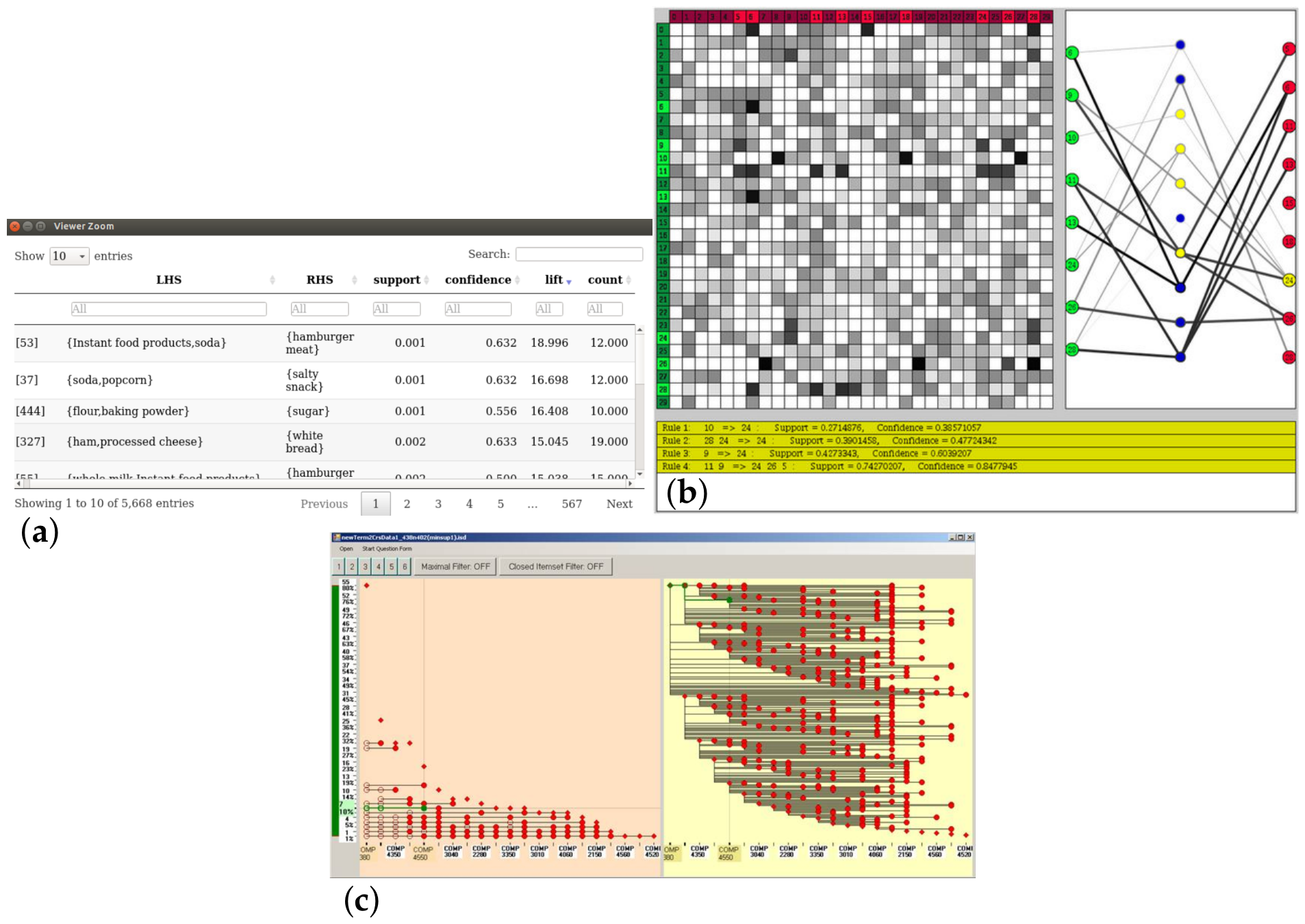
Different proposals for tabular representation can be seen in Figure 1. In particular, in Figure 1a we can find a table representation from the ArulesViz library [24]. With this representation, it is easy to see the rules and their measurements, and it is very simple to rank them according to the value of these measurements, support, confidence, etc. However, if the number of rules is large or if we want to explore the relationship of items or itemsets, the tabular representation is not ideal.

Another tabular way of representation is by means of a grid, where we can see the rules represented textually or using some edges to connect them. It is possible to observe these two different methods in Figure 2. The first is called Crystal clear [25], which allows the representation of the rules in an orderly manner according to their measurements. However, its main drawback is that you need to position yourself in the cell to discover the rule and its measurements, a process that makes it quite difficult and complex to explore the rules. Additionally, if the number of rules is large, we may find that the cells are too small.

In the second option, the tool used is WiFIsViz [26]. In this method, the rules are represented by some kind of tabular tree where items are placed in the axes. In this case, the relationship between consequent and antecedent is more intuitive. Moreover, the thickness of the nodes represents the measured strength of the selected rule (trust, support, lift…). This characteristic allows for better observation of higher value measurements more easily. In this case, the main drawback is that when the number of rules increases, the representation becomes very difficult to interpret and understand because the trees overlap in some nodes and edges.

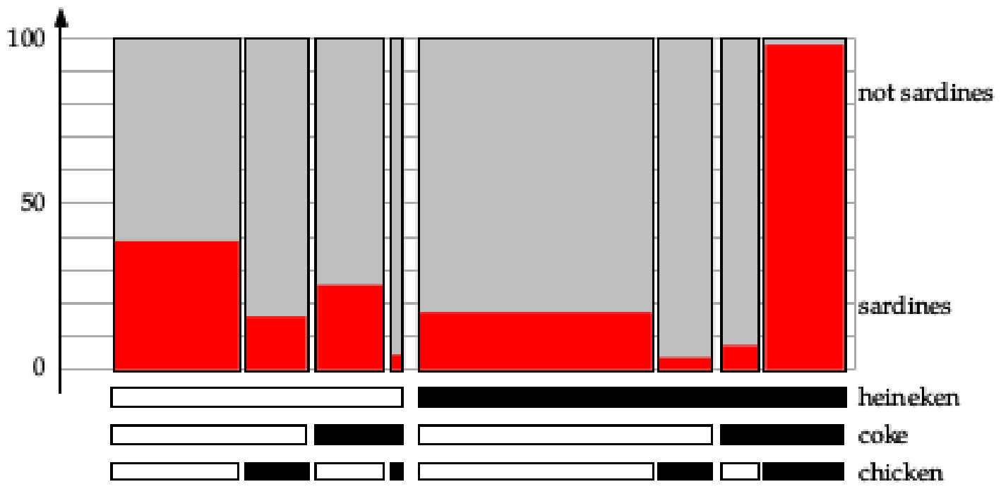
Figure 2. Example of mosaic plots for a set of rules [27]. where the height of the bar is to the indicated support between 0 and 100.

Figure 2. Example of mosaic plots for a set of rules [27]. where the height of the bar is to the indicated support between 0 and 100.

Another proposal can be found in [27], where the rules are represented in the form of mosaic plots. In this case, the way of visualizing the rules and their measure of interest is transformed through contingency tables. It can be observed in Figure 2 that this visualization method displays items more clearly and intuitively than the previous tabular-based visualization methods. Although its way of visualization works well for rules with few items, for many elements it quickly loses interpretability.

The main advantages of these types of tabular display techniques are their simplicity and ease of use, and the elimination of new evaluation measurements. This allows us to classify the results by their evaluation values. Because tables are a very common representation, they are generally very intuitive for any end user who wants to explore the results. Therefore, this is a convenient complementary option. They are also a good solution if we can filter, order and select rules from the results and use this kind of representation to explore them in more detail.

However, the major disadvantage of tabular representations is that they are not suitable for interpreting and understanding a large set of rules, as it is very difficult to observe all the rules and relationships between sets of items at the same time. Additionally, it is complex to see from a more general point of view the relationship between items through the rules or, for example, if there are groups of independent rules. So for these kinds of observations, we would need to use another type of representation.

3.1.2. Visualization of Parallel Co-Ordinates

Another common representation for representing rules is by means of parallel co-ordinates [28,29,30]. These were originally used to display relational records with an equal number of attributes. However, they can also be used to display data with variable lengths, such as frequent itemsets and association rules.

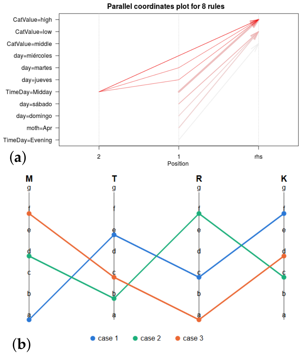
Some examples of such tools are found in [31,32,33] and can be seen in Figure 3. The tool developed in [24,33,34] can be observed in Figure 3a,b; it uses parallel coordinates to represent rules. The representation is based on axes (horizontal) with the items and a line (vertical) for each association rule. This line crosses the axes by the items/itemsets contained in the association rule. As we can see, it is a very descriptive and intuitive technique, but when the number of rules increases, it becomes complex to understand. Also, if the number of items increases, it is quite difficult to distinguish the rules that contain many items due to the amount of edges and connections generated (see Figure 3a). On the other hand, for smaller sets, this kind of visualization works with very good results, as we can see in Figure 3b. We can conclude, as in the previous group, that they are a good option to combine with other methods to visualize a specific set of rules.

Hence, the main advantage of this type of method is the simplicity and the ease of observing the relationship between the items. It is also very intuitive to understand how it works for small-size sets of rules by a person without any previous knowledge about the visualization tool.

However, these visualization methods become difficult to understand and interpret as the number of rules or itemsets grows. This is due to the fact that the representation of some rules is overwritten with others, which makes it complicated to determine which is each rule and which item belongs to the rule. In addition, we can also encounter problems when trying to visualize itemsets or rules with many items. In such cases, the problem is with following the long lines connecting items in the graph to determine which of them belong to the rule. On the other hand, when there are rules with many items, many lines have to be drawn, which makes the comprehension and representation of the rule quite difficult.

3.1.3. Matrix-Based Visualization

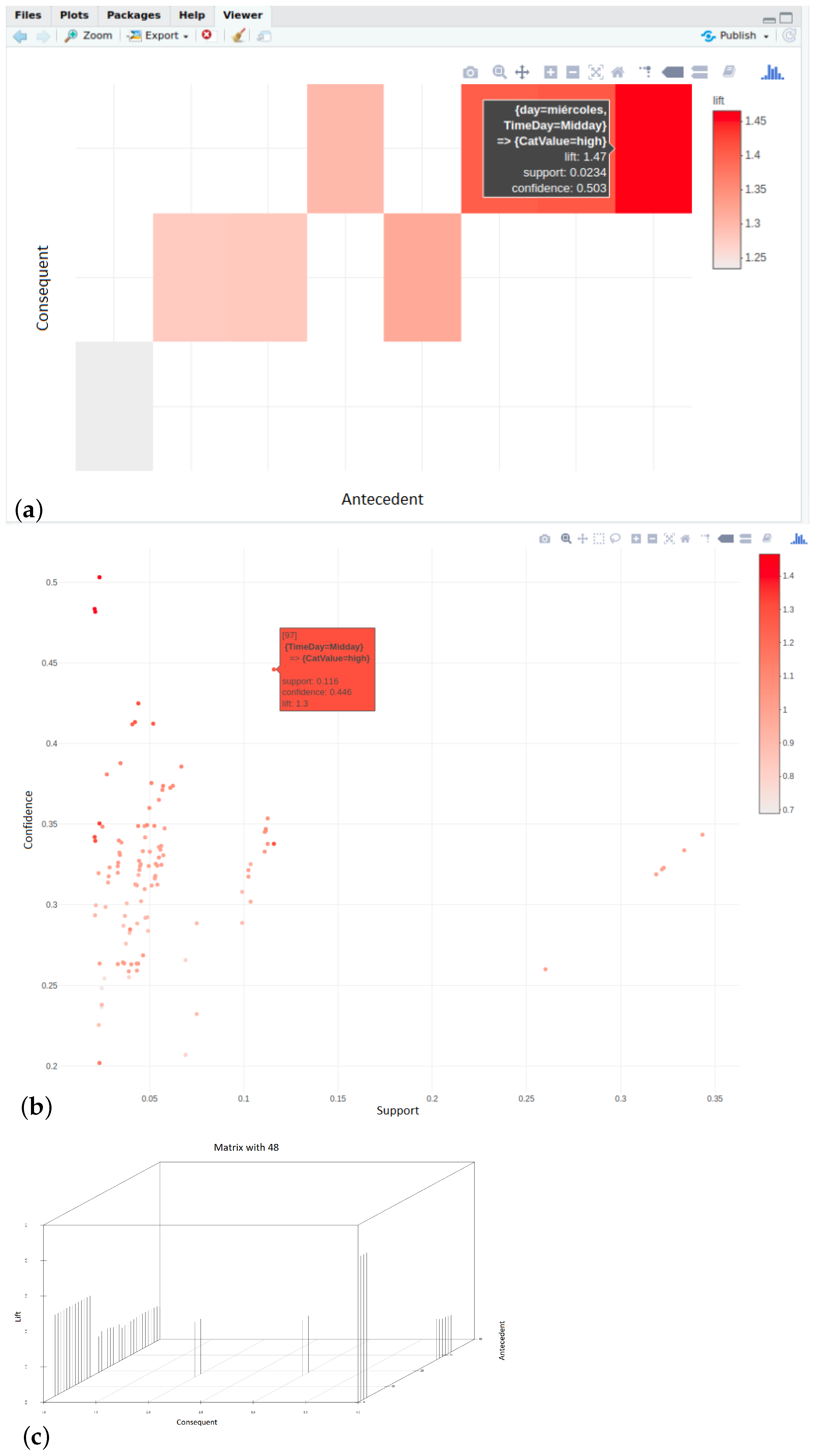
In the literature, we can find different tools that allow visualization through the use of matrices (2 or 3-dimensional). In Figure 4, we can see matrix-based visualizations using a scatter plot [35], a 2D matrix [27] or a 3D matrix [24,36].

In these techniques, the information to be visualized can be organized in two ways. Firstly, the rules can be displayed by antecedent and consequent in one of the axes (Figure 4a,c), and the measure of interest can be shown at the intersection of the antecedent and the consequent of the rules. At this point, there are different ways of representing it: using a third dimension and visualizing the measurement with, for example, a bar graph (Figure 4c) or by color intensity (Figure 4a,b). Some of these tools (e.g., a matrix plot in [27]) have an interactive component, and by positioning the mouse in the intersection that represents a rule, the user can see the different measurements related to that rule.

Another way is to display only the measurements (e.g., support and confidence) in the axes and to use an interactive box [37] to know which rules correspond to which pair of values. An example is shown in Figure 4b. In this case, if our interest is to explore the obtained rules by different assessment measurements, this type of visualization can be a good option.

When matrix-based visualizations use three dimensions, this allows a more general visualization of the set of results, helping to us know what the strongest rules are. These tools represent the rules in the following way: in the axes of the matrix, the items belonging to the consequent and to the antecedent are represented. In the intersection, a bar is drawn representing the measurements of interest.

One of the main advantages is that we can easily know which sets of items are more frequent, or which sets of items appear in more rules. In addition, these methods show this information along with the measurements of interest to improve our understanding of the results. These techniques can be customized in different ways using different colors, shapes or lengths. Also, if we want to see the whole set of rules in a general way, it is a suitable method because it allows us to see the related rules through the items and together with the value of their measurements of interest. For this, the best option is the 3D representation to observe easily and intuitively where the rules with the best measures are grouped.

However, this type of display has some disadvantages. First of all, it is very difficult to see the relationships between elements and rules when the set of rules/items is large. This is because when the set of items is very large, the axes of the matrix are heavily subdivided in such a way that it is impossible to differentiate which itemset corresponds to which rule. Similarly, if the number of rules is very large, the cells become very small and it is very complex to distinguish them.

3.1.4. Grouped Matrix-Based Visualization

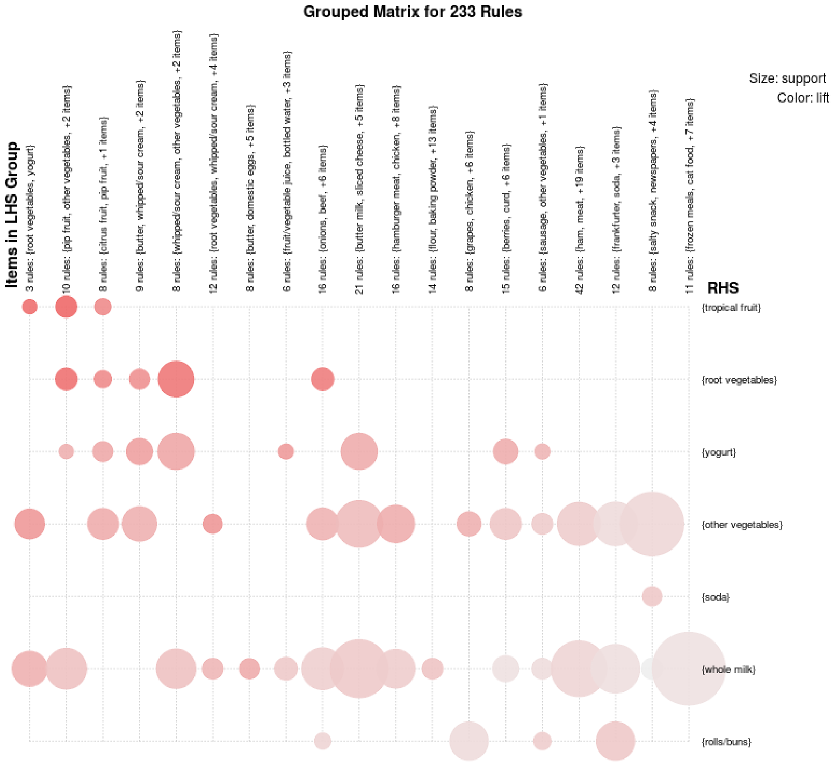
In this section, we explain a mixed technique named the grouped matrix-based visualization. In the previous case, matrix-based visualization tools were limited to the number of rules since they present difficulties when the number of items or rules increases [38]. Using the grouped version the relation between rules and itemsets can be better represented under these circumstances. In Figure 5 we can see an example of this type of visualization using the ArulesViz package [39].

Using this technique, the representation of rule sets with many items in matrices is improved because the tool groups the items. This technique is based on a representation in matrices where, on one axis, we have itemsets of the antecedents, and on the other, the consequent items; however, the represented rules can only have consequents with only one item. In this representation, the rules are grouped depending on the items of their antecedent, so for the same antecedent, several circles aligned with their respective consequent items can be shown.

Its main advantage is that it allows the visualization of large sets of rules. It is a good technique for analyzing rules by antecedent, since rules that have the same antecedent can be grouped. It is also an optimal representation to relate itemsets with the different classes, since it enables us to see the itemsets related to the same consequent.

Although it is a useful technique, its main weakness is that it cannot be easily adapted to display rules with more than one consequent. Additionally, this technique has problems when visualizing very frequent itemsets due to the size of the circles. In this situation, this kind of tool is not very useful, since very frequent rules fill almost all the available space.

3.1.5. Graph-Based Visualization

The graph-based displays consist of a transformation of the object to a structure of nodes and edges that connect the nodes. In addition, these elements can be associated with features to help the representation of more information within the network structure. In the literature, we can find different ways to transform rules into graphs [40,41]. One way is to represent each item as a node, and for each rule, add an edge to connect the items belonging to the rule. Additional features can be added, such as the color of the nodes, shapes, etc.

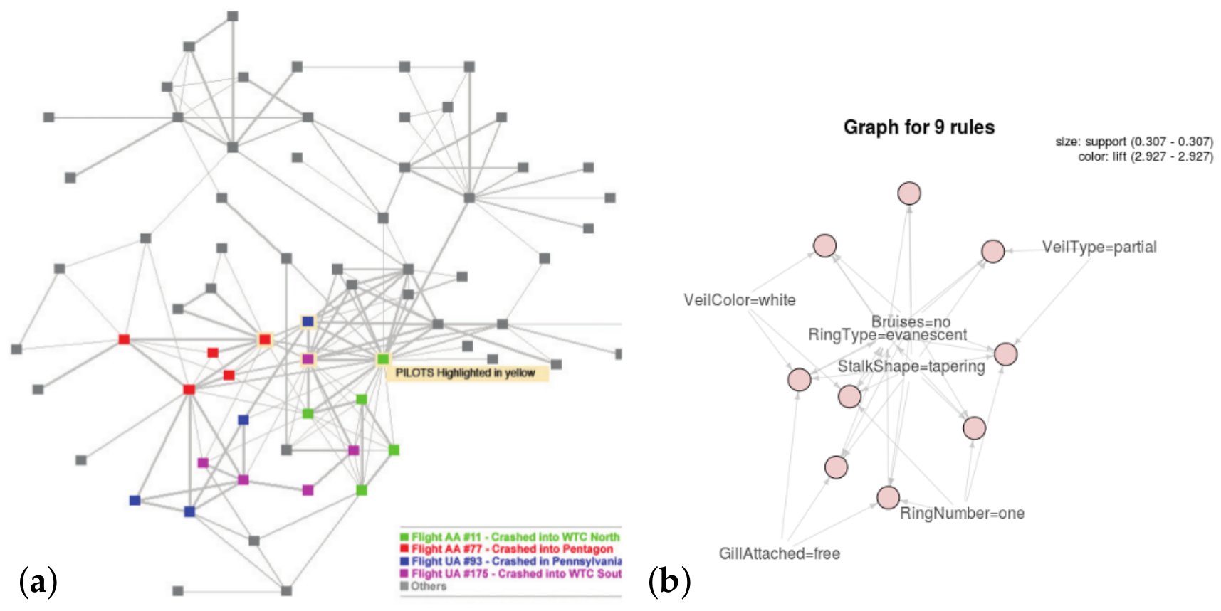
In the literature, there are different tools that make use of graphs to represent rules. Tools such as [42,43,44,45] allow a visual representation of the rules through some transformation into a graph. It can be seen in Figure 6 that with these tools, it is difficult to observe and intuitively understand the rules. Nevertheless, it is a good way to observe the general set of results. Moreover, as can be seen in Figure 6b, it is possible to represent large sets of rules. These tools can be enhanced with interactive capabilities, e.g. [44], where a subset can be selected or zoomed in.

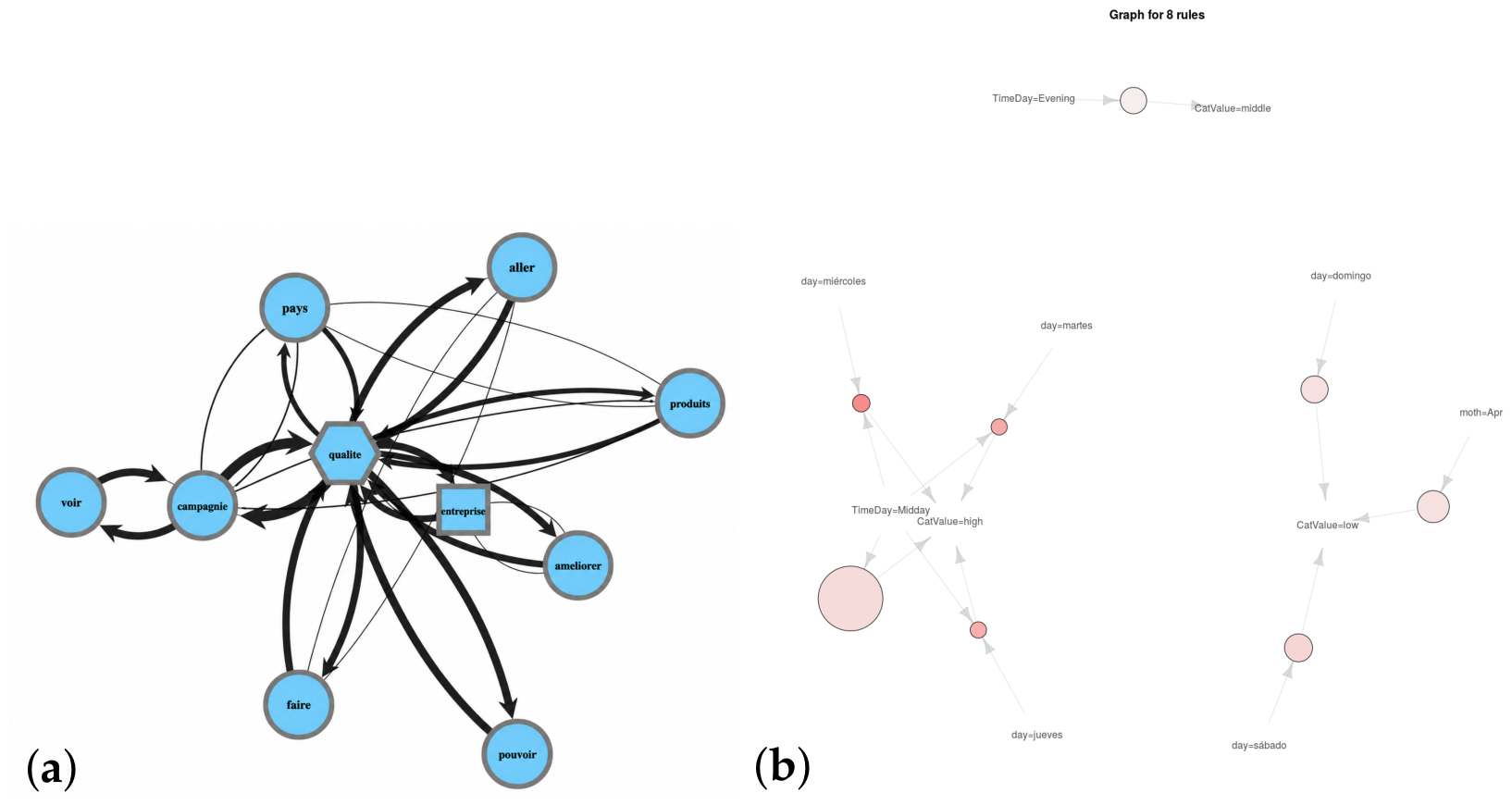
There are other tools oriented to graphs that use directed graphs [24,46]. These tools improve the interpretability and compression of the visualization because through the use of directed edges, we can know which node is the consequent or the antecedent (these tools are depicted in Figure 7a). We can observe that we can also represent measurements of interest of the rules by means of the forms of the nodes and edges. For example, in Figure 7b, the thickness of the edges and the size of the nodes are used, and the color intensity and the size of the nodes are used to represent the confidence and the lift assessment measurements.

As a result of the use of a graph structure, the visualization of the association rules can be improved by customizing the available design. Thus, increasing the interoperability for visualizing large sets of rules, and additionally, the graphical representation, is suitable for visualizing rules with various items in the antecedent and the consequent. On the other hand, this allows a more general vision of the set of rules by means of the size, color and form of the nodes and edges, as was the case for the matrix-based tools, for a better inspection of the rules, including assessment measures and the itemsets of the rules.

Nevertheless, graph-based visualizations have some drawbacks when working with large sets because, depending on the layout used, some rules are lost behind other rules. In addition, this type of visualization is not prepared to handle different measurements at the same time, since using more than two layouts (e.g., size and color intensity) to represent them may cause some confusion for the user. Moreover, these methods do not usually organize the items in a correct way, so it is more complex for the user to see the whole set of rules and interpret them. The use of interactive tools allowing the management of the graph as well as filter applications can greatly improve the inspection of rules represented by graphs.

3.1.6. Hybrid Approach

In this last group, we can distinguish different approaches to visualize rules using hybrid methods. They base their functioning on the use of different visualization methods in the same tool in order to try to strengthen their advantages and reduce their drawbacks.

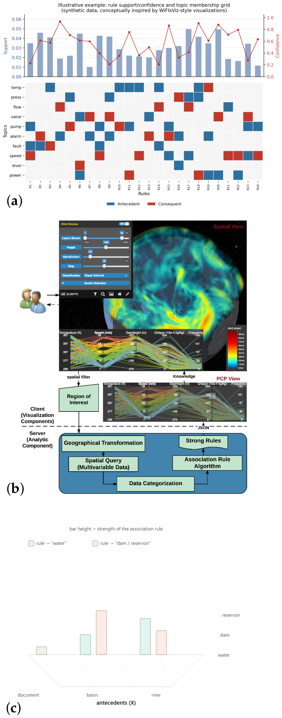
The proposal made in [36] (depicted in Figure 8a) uses a matrix to represent the rules and a bar diagram representing the support and confidence of each rule. The objective of this visualization is to address some disadvantages of matrix-based and grid-based tools. To do this, they combine a two-dimensional matrix and a grid to create a summarized view for a quick identification of the rules according to their levels of confidence and support. The main ability of the grid is to summarize the characteristics of a set of rules in a two-dimensional plane. Combining this with a bar visualization of assessment measurements in Figure 8a allows an analysis of rules based on the similarity of their antecedents and consequent characteristics. In this case, this visualization is more like a control panel where different aspects to inspect can be selected, and the most interesting rules. Figure 8a demonstrates the tool, specifically a 3D matrix representation for text mining. The rules are represented by a 3D box at the intersection, and depending on its color, it will represent the antecedent (blue) or the consequent (red) of the rule.

Other tools, such as the ones described in [42,47] (Figure 8b and Figure 8c respectively), use a dashboard to visualize, filter and select the rules to facilitate the search and extraction of information for end-users.

Figure 8. Hybrid-based visualizations (a) Illustrative example combining a support/confidence bar chart with an antecedent-consequent topic membership grid, conceptually inspired by hybrid rule-visualisation techniques such as WiFIsViz [26]. (b) Client-server architecture for spatial association rule visualisation, combining a heatmap-based spatial view, a parallel coordinates plot linked to the spatial data, and a backend workflow for geographical transformation, spatial querying, and association rule mining [48]. (c) Bar-based visualisation comparing antecedent items (e.g., document, basin, river) against consequent categories (e.g., water, dam/reservoir), where bar height encodes the strength of the association rule [47].

Figure 8. Hybrid-based visualizations (a) Illustrative example combining a support/confidence bar chart with an antecedent-consequent topic membership grid, conceptually inspired by hybrid rule-visualisation techniques such as WiFIsViz [26]. (b) Client-server architecture for spatial association rule visualisation, combining a heatmap-based spatial view, a parallel coordinates plot linked to the spatial data, and a backend workflow for geographical transformation, spatial querying, and association rule mining [48]. (c) Bar-based visualisation comparing antecedent items (e.g., document, basin, river) against consequent categories (e.g., water, dam/reservoir), where bar height encodes the strength of the association rule [47].

Another tool that combines different methods is [49]; in this case, the authors make use of a chord diagram. In the first, we can see an example with a lot of relationships, creating different chord diagrams depending on the attributes. The other two (b and c) represent sets of rules with fewer rules. This type of representation is very useful for appreciating the most frequent items appearing as consequent or antecedent items. However, it does not provide a good representation for large rule sets, although its combination with filters and other methods can be very useful (e.g., in combination with a matrix or graph-based representation to select groups of rules that are displayed afterwards in the chord diagram).

3.2. Classification by Type of Capacities of the Technology

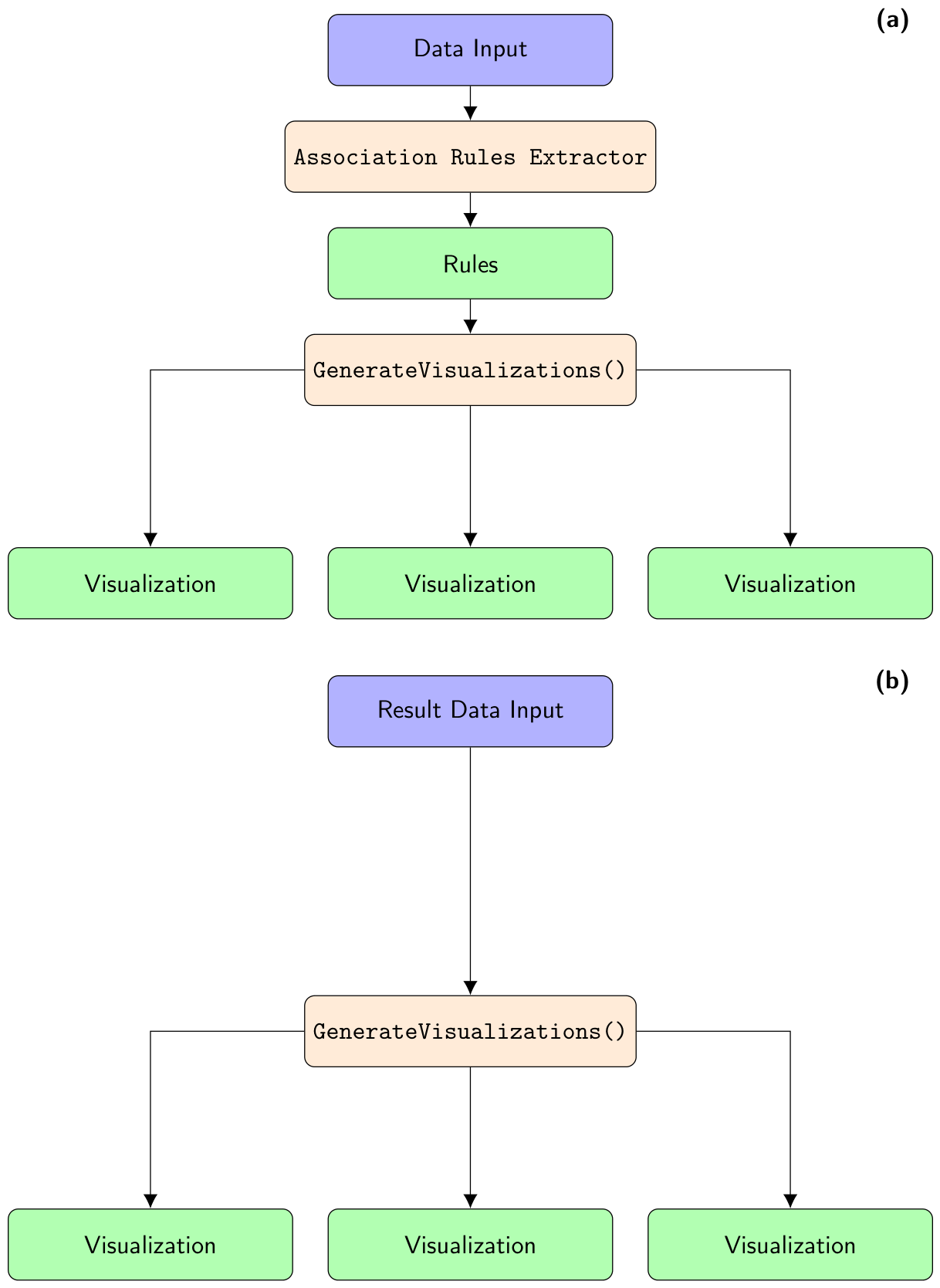
In order to visualize association rules, different types of tools can be found, depending on whether these only enable the visualization of the rules or carry out the extraction process of the association rules. According to this, we can classify them into two groups. On the one hand, there are tools that work as libraries that allow the extraction of frequent itemsets and association rules, and the visualization of the results (this process flow can be observed in Figure 9a). On the other hand, there are tools that allow the loading of the results obtained from other tools and then visualize them (this process flow can be observed in Figure 9b).

Within the first group of

Table 1. Comparative table of tools for visualizing association rules.

Name	Type Visualization	Type by Capacities	Focus	Advantages	Disadvantages
Arules Table [39]	Tabular 2D	Library Methodology	Measures Rule	-Intuitive -Easy to use -Show a wide variety of measures	-Problematic with many rules -Limited capacity with rules with many items -No overall view
CristalClear [25]	Tabular 2D	Visualization	Measures Rule
WiFIsViz [26]	Tabular 2D	Visualization	Freq. itemsets Rules
PEAR [52]	Tabular 2D	Library Methodology	Measures Rule
Arules Scatter plot [39]	Tabular 2D	Library Methodology	Measures set of rules
Arules Grouped Matrix [39]	Grouped Matrix	Library Methodology	Measures set of rules	-Displaying Large Rule Sets -Useful for rules with one consequent	-It is not possible to display rules with several items in the consequent -Not useful for sets with very freq. itemsets
Grouped Matrix [38]	Grouped Matrix	Library Methodology	Rules
Arules Matrix [39]	Matrix (2D, 3D)	Library Methodology	Rules	-Facility to explore items by measures -Possibility to visualize measurements by shapes, colors	-Difficult to scan itemsets in a rule -Problems when visualizing sets of many items (insufficient axis length) -Overview of the whole (interactive tools improve this point)
Matrix [35]	Matrix (2D, 3D)	Library Methodology	Rules
Matrix for text mining [36]	Matrix (2D, 3D)	Library Methodology	Rules
Arules interactive Matrix [37,39]	Matrix (2D, 3D)	Library Methodology	Rules
Mosaic plots [27]	Tabular 2D	Visualization	Freq. itemsets Rules	-Better compression of the relationship between items -Possibility of using colors to visualize measurements	-Complexity in using rules with many items -Only for reduced sets of rules -No overall view
ArulesViz [39]	Graph	Library Methodology	Items	-Wider vision as a whole -Possibility to apply different layouts -Ability to view large rule sets -Interactive -Ability to view rules consistent with various items -Use of color, shape, directionality on edges and nodes to express rule measurements	-Large sets of rules result in many nodes and edges, so it is necessary to select a good algorithm of layouts for the visualization and interpretation are correct -Not prepared to handle different measurements at the same time -More complex for the user because it is necessary to know the structure of a network and how represented the rules are in it -Some of them are difficult to interpret
VisAR [34]	Graph	Visualization	Freq. itemsets Rules
Criminal Network [42]	Graph	Visualization	Freq. itemsets Rules
Product network analysis [43]	Graph	Visualization	Freq. itemsets Rules
Projection Explorer [44]	Graph	Visualization	Freq. itemsets Rules
Spanning trees [45]	Graph	Library Methodology	Freq. itemsets Rules
SYSNETS [46]	Graph	Visualization	Freq. itemsets Rules
RDViz [53]	Graph	Library Methodology	Rules
WiFIsViz [26,47]	Graph	Visualization	Freq. itemsets Rules
Arules Tow-key plot [39]	Tabular 2D	Library Methodology	Rule length	-Simplicity -Ease to observe relationships between items -Easy and intuitive understanding without knowledge	-Difficult to represent the measures of the rule -Problems when increasing items or number of rules -Better for rules with few related items
Parallel Coordinates [33]	Parallel Coordinates	Visualization	Measures Rule
Parallel Coordinates [32]	Parallel Coordinates	Visualization	Measures Rule
Parallel Coordinates [24]	Parallel Coordinates	Library Methodology	Measures Rule
CristalClear [25]	Hybrid: -Graph -Chord -Tree	Visualization	Measures Rule	-Observation as a whole and on concrete rules using various methods -Interactive -Selection and filter combining methods -Diversification of measures to improve the exploration of the results	-For specific use cases -More complex management tools with many filters and interactions between displays -In some cases it is necessary to have certain data such as geolocation, temperature data because the displays are developed for those data
Visual discovery of network patterns [49]	Hybrid: -3D Matrix -Bar diagram	Visualization	Freq. itemsets Rules
Hierarchical visualization [47]	Hybrid: -Chord -Graph	Visualization	itemsets Rules
Criminal visualization [42]	Hybrid: -Chord -Graph	Visualization	Freq. itemsets Rules

, we find different methods that allow us to load the results obtained with extraction tools for association rules. These must be loaded using a different standard structure depending on the tool used to be able to visualize them. Amongst them we can highlight several tools [27,31,32,36,49,50,51] that, from the stored results as association rules, allow us to visualize the rules in different ways (which are described in more detail in Section 3.1).

In the second group of the Table 1, we find methods that enable complete analytical procedures from the same tool. For example, in the Arules package [24], we can extract frequent itemsets and association rules to later visualize them by making use of this library. PEAR works in a similar way; it follows the methodology developed in [52] allowing the whole process to be performed, from the loading of data to the visualization. Its main difference is the use of a set of rules, through the use of operators that allow us to unify these rules by grouping them into sets. This new set of rules can then be displayed with the available methods.

3.3. Comparison of Standards in the Representation of Association Rules

Before presenting our proposal, we review the different literary standards for association rules to study their suitability for use in visualization. Table 2 summarizes the different features of the available standards that are used for storing association rules.

3.3.1. Tabular

These formats are widely used for data science models. The tabular format, such as CSV or TSV, is widely used by many tools and can be viewed natively via various tools. However, it does not allow us to extract all the information contained in the relationships among items. We can see an example of this problem in the tabular visualization (native visualization of tabularly stored files).

This type of storage needs preprocessing and transformation to be able to visualize it with other tools in order to extract all the information contained in the results of the association rules.

3.3.2. PMML

The Predictive Model Markup Language (PMML [54]) model supports the representation of frequent itemsets and association rules that can be useful for frequent itemsets or association rule results. The PMML provides a representation model comprised of four major parts:

• Model attributes: information regarding the model, whether they are association rules or frequent itemsets, in addition to the assessment measures used, e.g., support, confidence and other parameters.
• Items: items contained in the model
• Itemsets: itemsets stored in the results
• Association Rules: association rules obtained by the algorithm

An AssociationModel (see the example in the documentation [55]) can contain any number of itemsets and association rules, provided that all itemsets, composed of items, are listed before any rules. Nevertheless, there are a number of limitations for the representation:

• It does not contain all the metadata about the experimentation done. It would be useful to have some metadata about the experimentation like the date and time stamp, name of the database employed, etc.
• It is not flexible/dynamic enough to include other types of association rules, like fuzzy rules, or other assessment measures different from those taken into account in the standard.
• The file generated using the PMML format can be very large when many association rules are managed.

Another limitation is related to the fact that Association Rules are both a model and the output of a Knowledge Discovery mechanism.

Table 2. Comparative table of standards for association rules.

Name	Type	Type by Capacities	Focus	Advantages	Disadvantages
PMML [54]	XML	Standard format	FreqItems Rules	-It is widely used for different models used in data science -It has examples and great documentation -It is used by some libraries for exporting their results (Arules in R)	-It does not contain all the metadata about the experimentation done -It is not flexible/dynamic enough to include other types of association rules like fuzzy rules, or other assessment measures different from those taken into account in the standard -The file generated by using the PMML format can be very large when many association rules are managed
JGF [56]	JSON	Standard format	FreqItems Rules	-It allows the representation of a wide range of visualization tools -Widely known format for the representation of information as entities	-Need to adequately represent the entities to be represented -Need to design an efficient structure that allows the representation, reading and visualization of the information
Tabular Data	XML	Standard format	FreqItems Rules	-It exploits the benefits offered by eXtensible Markup Language (XML) specifications and related tools in order to model a fuzzy logic system	-Not efficient for large result sets -Need to parse data to use most visualization tools -Very specific to one type of model

Table 2. Comparative table of standards for association rules.

Name	Type	Type by Capacities	Focus	Advantages	Disadvantages
PMML [54]	XML	Standard format	FreqItems Rules	-It is widely used for different models used in data science -It has examples and great documentation -It is used by some libraries for exporting their results (Arules in R)	-It does not contain all the metadata about the experimentation done -It is not flexible/dynamic enough to include other types of association rules like fuzzy rules, or other assessment measures different from those taken into account in the standard -The file generated by using the PMML format can be very large when many association rules are managed
JGF [56]	JSON	Standard format	FreqItems Rules	-It allows the representation of a wide range of visualization tools -Widely known format for the representation of information as entities	-Need to adequately represent the entities to be represented -Need to design an efficient structure that allows the representation, reading and visualization of the information
Tabular Data	XML	Standard format	FreqItems Rules	-It exploits the benefits offered by eXtensible Markup Language (XML) specifications and related tools in order to model a fuzzy logic system	-Not efficient for large result sets -Need to parse data to use most visualization tools -Very specific to one type of model

3.3.3. JSON Graph Format

The JSON Graph Format [56] allows the results to be represented as a graph, enabling the relationships between different itemsets to be expressed directly. However, this is a general framework for graph representation, and it is not suitable for association rules. In order to take advantage of all the benefits of this format, we present in the next section an intermediate form to improve the representation of association rules, which is compatible at the same time with the majority of the available visualization libraries.

3.3.4. Discussion

There are many tools that allow us to visualize association rules. However, all these techniques are independent of each other and use different formats for the rule extraction and for the use of results to display them. In addition, the methods that enable the complete process from the rules extraction to the visualization have some problems because they do not allow the use of other methods for visualization or extraction. This is why we propose a methodology using an intermediate form with the purpose of improving the interoperability, which will be able to use different visualization methods by transforming the rules into an intermediate form that can be used in a wider range of visualization tools.

Therefore, the chosen format should:

• Be compatible with the visualization library (in general, this will be graph visualization).
• Preferably also be in a format that makes it possible for a human expert to quickly scan the set of association rules discovered.

4. Our Proposal: A New Methodology Using an Intermediate Form

We present in this study a novel methodology with the purpose of facilitating and improving the process of extraction, standardization, and exploitation of results, thus enabling the use of the existing libraries in the literature.

As we have described above, the available standards in the literature allow the storage of frequent association rules and itemsets, but in an inefficient way. Also, their structure cannot be directly employed to use the visualization tools described in Section 3. This new proposal solves these problems. It consists of representing the rules through an intermediate form that allows the use of different tools to visualize the results, as well as a more efficient structure for their storage and the possibility of carrying out searches or transformations on them.

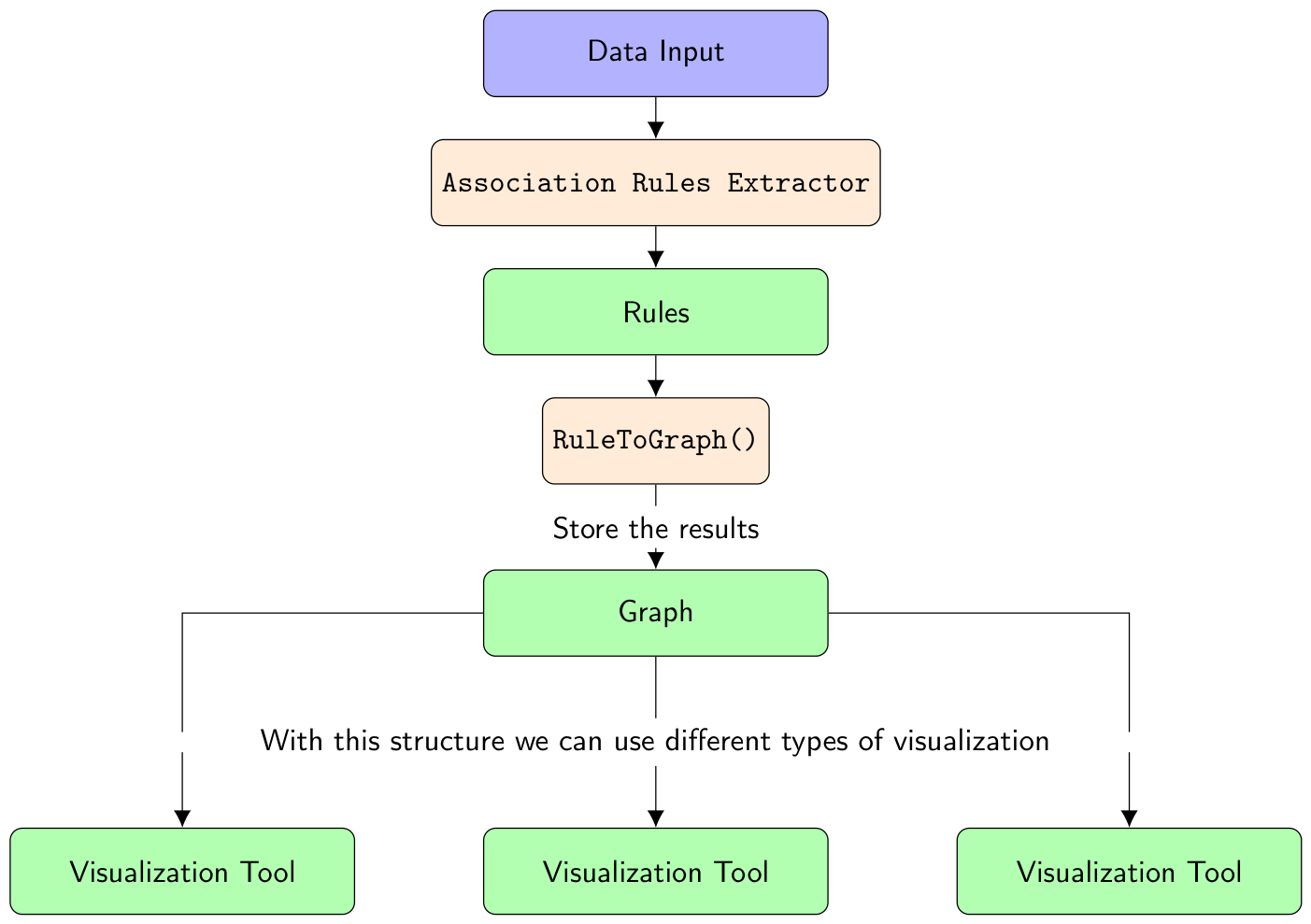
Our proposed methodology is based on a transformation of the rules into a graph, adding different capabilities to improve their display. As we have seen in the previous section, the JGF format allows us to represent information as a graph in an efficient way and is easily natively interpreted by a variety of visualization tools. The procedure we followed to make a visual representation of the association (depicted in Figure 10) can be divided into three phases.

The first one is in charge of obtaining the rules by means of association rule mining algorithms. Next, we transform and process these results into a graph representation. The final step is the visualization of this structure, which enables the visualization of the rules using different tools.

On the one hand, the proposed intermediate form provides a format to store the results obtained from the association rule mining process that allows consultation and efficient filtering by means of the elements and measurements associated to the rules. For example, it is possible to store the results natively in NoSQL databases, from which we can then display them using visualization libraries such as Bokeh, Arules or 3D.js.

Finally, this methodology is generic because it is applicable in tools such as those that use a workflow such as the one shown in Figure 9b, which perform the extraction of the rules and then the visualization. This improves not only the visualizations that a tool implements but also the possibility of being able to use the intermediate form to use visualizations of other tools. On the other hand, in the case of the tools following the pipeline of Figure 10, this enables a generalization of a visualization technique for any association rule extraction algorithm.

4.1. Transformation of Association Rules into a Graph

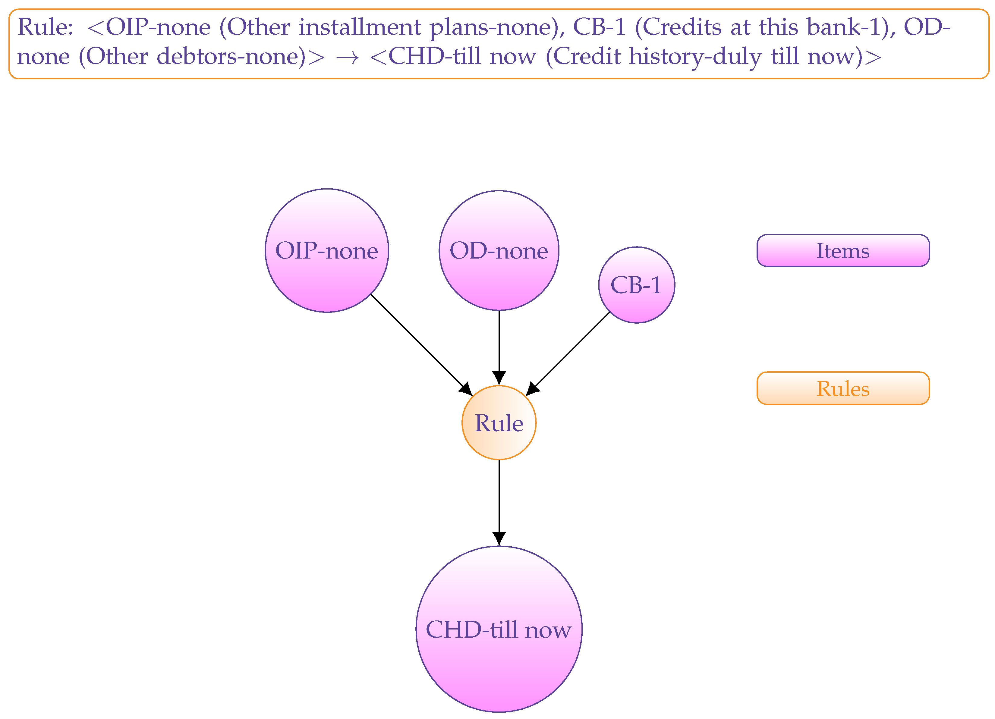
The first step before visualizing the rules is to transform them into a graph; there are different options to do this. In our case, we perform a transformation to a graph made up of two types of nodes: items and rules. The nodes will be connected according to the results that have been obtained. To better explain the functioning of the graph transformation, we have constructed an example by extracting association rules from the German Credit Data (excluding continuous attributes) from the UCI Machine Learning repository [57]. We can see in

Table 3. Set of association rules obtained for the German-statlog database.

Antecedent	Consequent	Supp	Conf
(Other installment plans—None) (Credits at this bank—1) (Other debtors—none)	(Credit history—duly till now)	0.37	0.7822
(persons maintained—1) (Job—skilled) (Other installment plans—None)	(Other debtors—none)	0.427	0.9085
(Housing—own) (persons maintained—1) (Credits at this bank—1) (Credit amount—0–3000)	(Credit history—duly till now)	0.31	0.7944
(Housing—own) (Other installment plans—None) (Credit history—duly till now)	(persons maintained—1) (Other debtors—none) (Credits at this bank—1)	0.22	0.7229
(Housing—own) (Credit amount—0–3000) (Credit history—duly till now)	(Credits at this bank—1) (persons maintained—1)	0.21	0.8104
(Savings account—less100DM) (Job—skilled) (Foreign worker—yes)	(Other installment plans—None)	0.206	0.8512
(Credit amount—0–3000) (Credits at this bank—1)	(Other debtors—none) (Other installment plans—None)	0.29	0.7430

the set of selected rules that will be used in the different examples below. Figure 11 shows an example of a rule transformed into a node that connects the item-type nodes.

Algorithm 1 describes the procedure for transforming a set of rules into a graph. The transformation is performed for each rule of the database, and carried out taking into account the corresponding associated characteristics according to the type of node rule of the item. For example, for a rule type, the node will contain information about the measures of interest (e.g., support, confidence, lift). Then, in line 14, the edges of the graph are added, taking into account the type of link (whether it is the consequent one or an antecedent). When this process ends, the rules are represented by a graph through which we can make different types of display.

Algorithm 1 Main transformation procedure for Rules to Graph

1: Input: Data: a csv/RDD containing the rules.   2: Output: Graph for association rules exceeding MinSupp   3: Rules = ReadData()   4: Graph = {}   5: for $n=1;NumberofRules;n=n+1$ do   6:       $Antecedent,Consequent\leftarrow SplitRule\left(Rules\right[n\left]\right)$   7:       if $not\left(AntecedentinGraph\right)$ then   8:             $Graph.Ad{d}_{Node}\left(ConvertToNode\left(Antecedent\right)\right)$   9:       end if 10:       if $not\left(ConsequentinGraph\right)$ then 11:             $Graph.Ad{d}_{Node}\left(ConvertToNode\left(Consequent\right)\right)$ 12:        end if 13:        $Graph.Ad{d}_{Node}\left(ConvertToNode\left(RuleN\right)\right)$ 14:        $Graph.Ad{d}_{Edge}(RuleN,Antecedent,Consequent)$ 15: end for 16: $Return\leftarrow Graph$

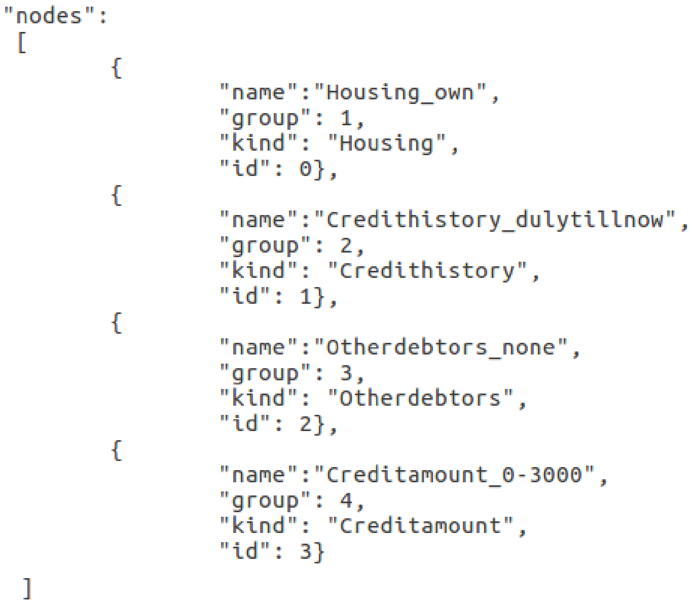
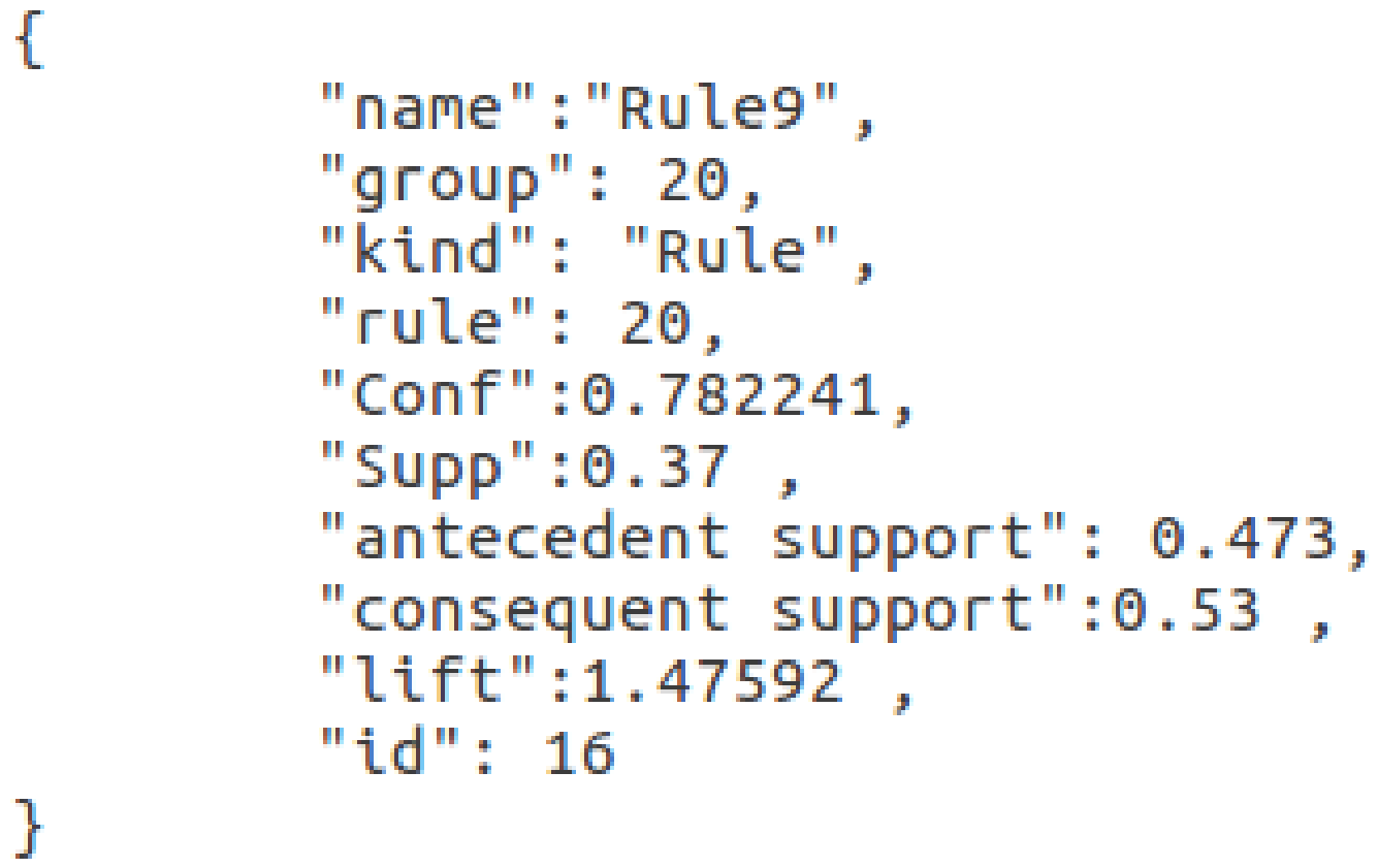
Figure 12 exemplifies the structure followed for representing an item node. In this case, the name indicates the pair ‘atribute_value’ that represents the item; the group and kind represent the attribute name of the item or whether it is a node of rule type (see Figure 12). The group number is used to improve the efficiency in some types of visualization such as graphs. Finally, node id used for univocally identifying the node.

On the other hand, in Figure 13 we can see the structure for nodes representing a rule in the graph. In this case, this type of element also stores the measures related to the rule such as support, confidence, etc. This generated structure allows a later visualization of the obtained rules in a way that improves the interpretability and comprehension of the results.

Proposed Intermediate Format and Syntax

The proposed intermediate format is based on a structured JSON schema that encodes association rules as a typed graph composed of two differentiated entities: item nodes and rule nodes, together with directed edges that represent antecedent and consequent relations. This representation is designed to be both machine-efficient and human-interpretable, while remaining directly exportable to document-oriented and graph databases. Each node definition follows a fixed syntax with mandatory fields. All nodes include a unique identifier (id), a human-readable label (name), a categorical grouping field (group) used for visualization and indexing, and a kind attribute that specifies the node type (item or rule). Item nodes encode atomic attribute–value pairs using the normalized syntax attribute_value, ensuring consistency and avoiding ambiguity across datasets. Rule-type nodes extend the base syntax with a set of quantitative quality measures, such as support, confidence, lift, and optionally additional metrics (e.g., leverage or conviction). These measures are stored as numeric fields, enabling direct filtering, ranking, and threshold-based queries without additional parsing. Edges are represented as directed links with explicit semantic roles. Links from item nodes to rule nodes are labelled as antecedent relations, while links from rule nodes to item nodes are labelled as consequent relations. This directional syntax preserves rule semantics and allows rule decomposition and traversal using standard graph queries. Overall, the proposed syntax defines a minimal but extensible schema that guarantees univocal identification, typed structure, and metric-aware storage.

4.2. Rule Summarization via Graph Abstraction

A central limitation of storing and visualizing association rules as a flat list (or as a graph containing one rule node per discovered rule) is that the number of rules can grow rapidly with dataset size, support thresholds, and item granularity. In such regimes, direct inspection of individual rules becomes computationally and cognitively demanding, and many existing visualization techniques degrade due to node/edge clutter. Therefore, beyond interoperability, we require a formal mechanism that provides a compressed representation of the rule set while preserving the ability to drill down into the underlying rules when needed.

We introduce an optional summarization layer that operates on the intermediate typed graph produced by the RulesToGraph transformation. The summarization step replaces subsets of rule nodes by summary nodes representing rule groups that are equivalent under a user-defined signature (e.g., identical antecedent sets, identical consequent sets, or identical antecedent–consequent signatures). This yields a hierarchy that supports progressive disclosure: summary-level exploration first, followed by fine-grained inspection at the original rule level.

Let $\mathcal{R}$ be the set of extracted rules, and let each rule $r\in \mathcal{R}$ be associated with: (i) an antecedent itemset $A\left(r\right)$, (ii) a consequent itemset $C\left(r\right)$, and (iii) a vector of quality measures $m\left(r\right)$ (e.g., support, confidence, lift). We define a grouping function $\sigma (·)$ that maps a rule to a discrete signature. Examples include:

$${\sigma }_{\mathrm{A}}\left(r\right)=\mathrm{hash}\left(A\left(r\right)\right),{\sigma }_{\mathrm{C}}\left(r\right)=\mathrm{hash}\left(C\left(r\right)\right),{\sigma }_{\mathrm{AC}}\left(r\right)=\mathrm{hash}(A\left(r\right)\cup \{\to \}\cup C\left(r\right)).$$

For each signature s, let ${\mathcal{R}}_s=\{r\in \mathcal{R}:\sigma \left(r\right)=s\}$. We create a summary node $S_s$ for each non-empty ${\mathcal{R}}_s$.

For each aggregated quality measure $m\in \{\mathrm{support},\mathrm{confidence},\mathrm{lift},\dots \}$, we store a compact statistic bundle in $S_s$, including: (1) $|{\mathcal{R}}_s|$ (number of member rules), (2) ${\max }_{r\in {\mathcal{R}}_s}m\left(r\right)$ and ${\min }_{r\in {\mathcal{R}}_s}m\left(r\right)$, (3) ${\mathrm{mean}}_{r\in {\mathcal{R}}_s}m\left(r\right)$, and (4) optional quantiles (e.g., $Q_{0.25},Q_{0.5},Q_{0.75}$). Additionally, the summary node maintains a membership list of the rule identifiers $\mathrm{members}\left(S_s\right)$ to enable drill-down visualizations.

The intermediate JSON schema is extended to include a new node type kind: “summary”. Summary nodes participate in the same typed graph, connected to item nodes (or to signature-derived item representatives) in the same directed semantic direction as rule nodes. Visualization tools can then either (i) render the full rule-level graph, or (ii) render the aggregated summary-level graph to avoid clutter, depending on a user-selected granularity.

This summarization layer constitutes a formal, schema-integrated aggregation mechanism that complements the intermediate-format contribution. It explicitly addresses scalability by replacing sets of individual rules with aggregated nodes, enabling interpretable visualization of large rule sets without sacrificing traceability to the original rules.

4.3. Intermediate Form Storage

Generally, rules do not have a predefined structure for storing them that enables a fast retrieval or efficient navigation. By using the intermediate form we can store our results in different database formats such as MongoDB or Neo4j. These types of databases are especially designed for rapid filtering and sorting by order, allowing flexible and dynamic schemes.

Thanks to this structure, the rules stored following this type of JSON representation can be efficiently searched and retrieved by their measures of interest (in MongoDB by indexing the rules or in Neo4j by looking only for the type of node rule). Besides this being a standard format, exporting into databases is direct and very efficient (in MongoDB, the native format is BSON a derivative format of JSON). On the other hand, if we use Neo4j, we will also have the capability of querying graphs using its Cypher query language.

Finally, the intermediate form also makes it simple to query the results of association rules using standard query APIs such as GraphQL. This natively allows the querying of stored results by using the intermediate form in a database.

4.4. Visualization Tools

Having transformed the rules to a graph structure following the methodology described in Figure 10, we can make use of the intermediate form to use different visualization tools, some of which we have already described in Section 3.

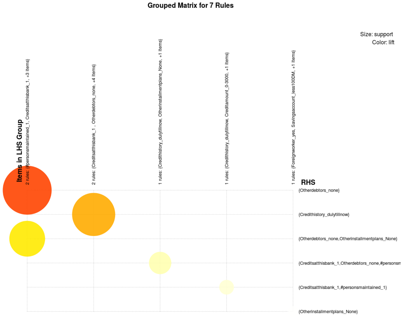
Taking into account the above mentioned structure, we can use different graph visualization libraries such as Gephi [58], D3JS [59], Bokeh [60], ggnet2 [61], NetworkX [62], NOESIS [63], etc. These tools return a graphical display of the transformed rules. In addition to these graphical visualization tools, we can use other libraries such as Arules as we can see in Figure 14, where we have employed the set of rules from Table 3. Thanks to the use of our methodology, we can visualize rules with more than one consequent (the rule extraction algorithm of the Arules package only allows rules of only one consequent) using an external algorithm [64] and using the intermediate form previously explained.

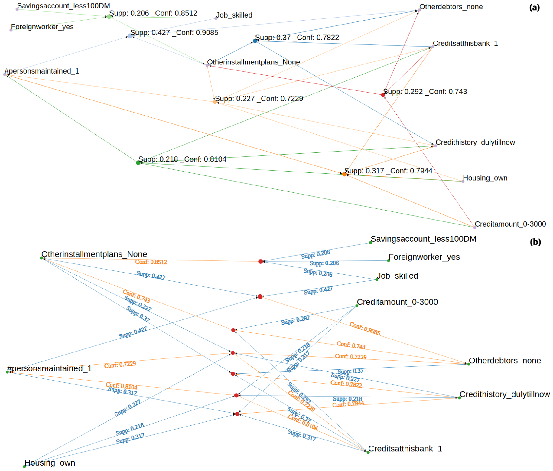
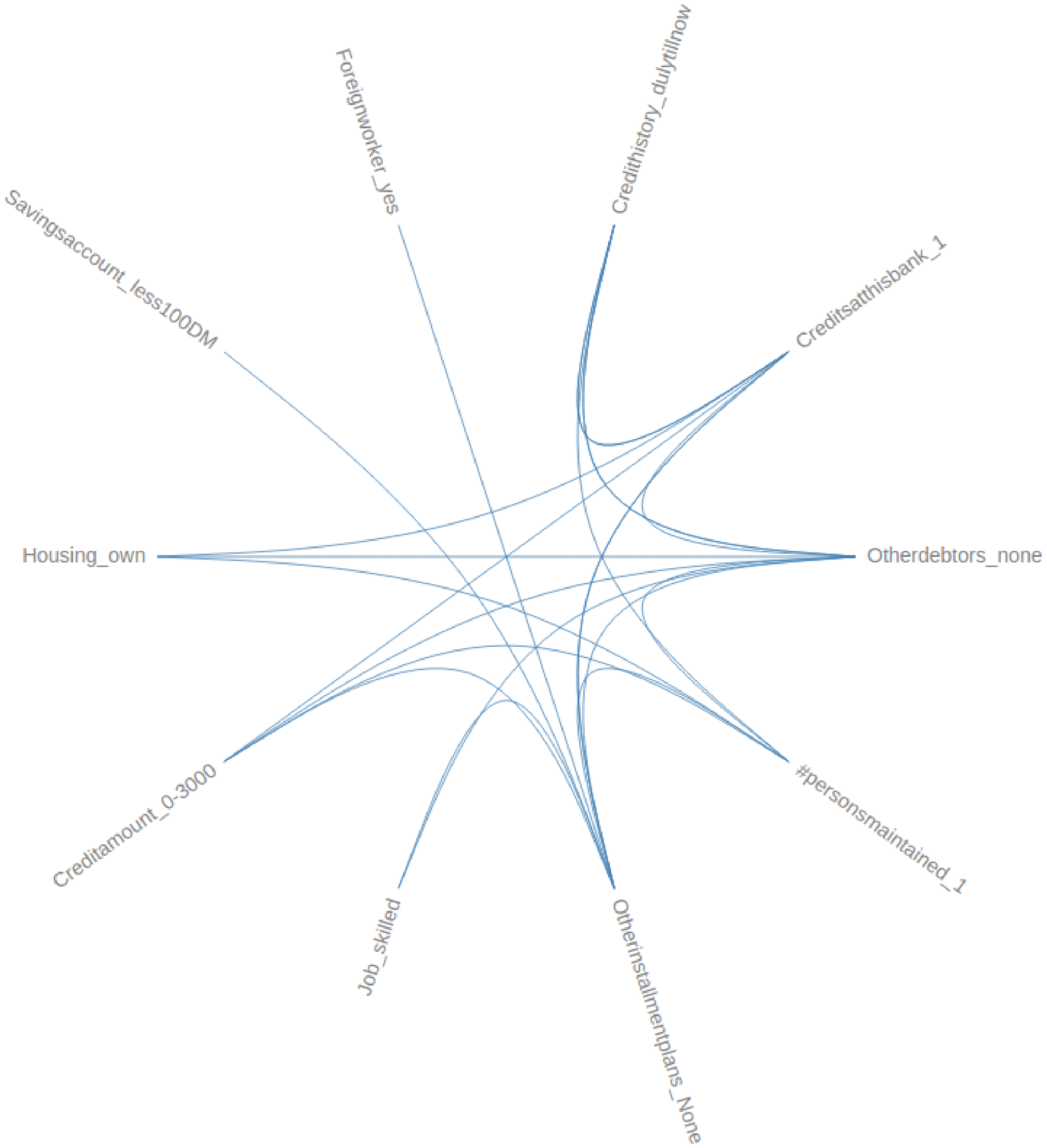
Moreover, we can use libraries and visualization tools to customize exiting visualization tools to adjust according to user preferences. A powerful visualization package enabling this kind of modification is 3DJS [59]. For example, in Figure 15, we have adapted a graph-based display called a Force-directed graph, where a different color is used for each rule, and every node of the type ‘Rule’ shows the associated support and confidence of the rule. Additionally, the directionality of the arrows to the rule node indicates whether an item node is part of the antecedent (arrows pointing to the rule node) or part of the consequent (arrows pointing to the item node). A variation of the previous visualization is also made in Figure 16 where we have customized some properties of the graph, such as indicating the item support in the edge. Another example is the chord diagram shown in Figure 16, also customized from making use of the 3DJS library. This visualization is interactive: when you are positioned in the items, the edges are emphasized and colored according to the relationship they have with other items (antecedent or consequent).

With respect to the efficiency and scalability of the visualizations on graphs, the developed tool is able to generate the graphs in SVG format (Scalable Vector Graphics), thus allowing it to be distributed by means of the Tuoris library [65].

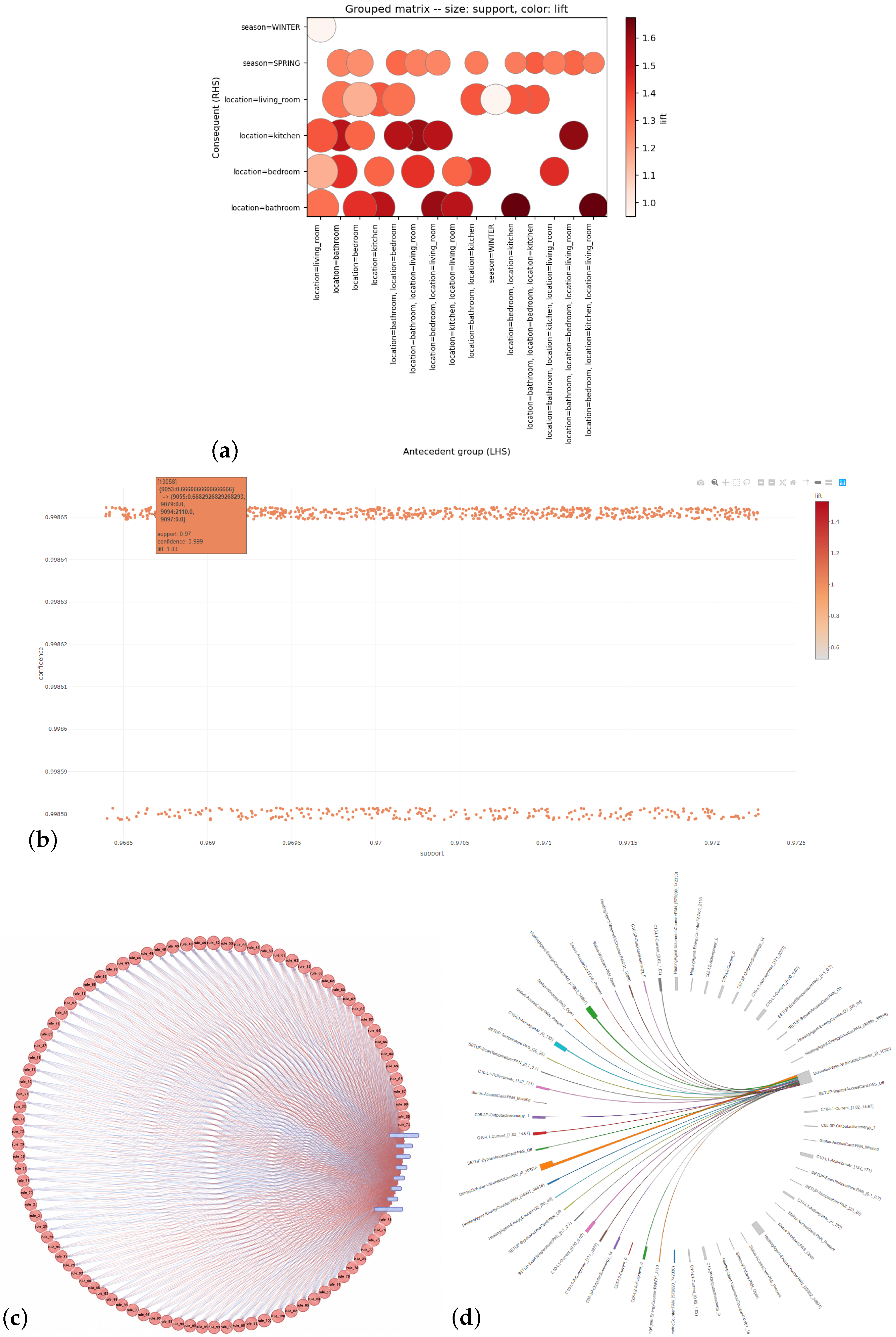
It is worth mentioning that this intermediate form allows the efficient storage of results and their visualization by different tools. Here is an example of a dataset of 4 million records and 4567 sensors from an office building in Romania. This example has been carried out with an association rule extraction tool in Big Data and 77,812 rules were obtained. In Figure 17, we can see different rules filtered and visualized with different tools using the intermediate form.

5. Discussion

In this paper, we have reviewed the most commonly used methods to visualize association rules. From the different tools examined, we have seen that each one comes with strengths and weaknesses. As part of this analysis, we have been able to see that there is no one display tool that works well for all cases. This is because, depending on the problem, the dataset and the objective, we need to choose the best visualization solution for our requirements. Furthermore, we have reviewed the most common association rule storage standards and found that none of them are widely compatible with all the visualization tools, and they also present major efficiency problems when they contain large sets of rules. In addition, some of the tools allow the exportation of data from our own algorithms and others do not; therefore, it is necessary to have a standard format with which to exchange our results amongst the different tools in order to exploit the strengths of each tool and add interoperability to the process. Thus, we would be able to have more resources and not depend on a single tool to get a better visualization and understanding by the end user. Therefore, our proposal will allow us to extract the association rules from any algorithm or from a library and then export it to be displayed using the different available libraries: 3D.js, Arules, Bokeh, etc. Furthermore, this standard and widely known format can be stored natively in databases that allow efficient filtering, search and storage of large sets of results.

6. Conclusions and Future Research

To sum up, we have carried out an extensive analysis of the different visualization tools available in the literature, as well as classifying them according to the type of visualization and the capabilities they offer. As a result of this analysis, we have seen that most of the tools only allow the visualization of rules from a predefined structure, or the library containing the visualization only allows the generation and display of rules through their own algorithms. Therefore, in these cases, the user cannot combine their own or other available association rule mining algorithms with available techniques to be able to present association rules in a graphical way.

Because of this, in this paper, we put forward an intermediate representation that allows the use of a great variety of the tools for association rules, and in addition, it allows us to combine them with the different available visualization techniques.

Regarding future research, we aim to implement a complete open-source library for the extraction of the rules and transformation into the intermediate form. In addition, our purpose is to implement this intermediate form in a modular way in order to have APIs between modules and to enable the use of different association rule extraction algorithms, with this representation thus facilitating the connection with available visualization libraries.

References

1. Agrawal, R.; Srikant, R. Fast Algorithms for Mining Association Rules in Large Databases. In Proceedings of the 20th International Conference on Very Large Data Bases (VLDB ’94), San Francisco, CA, USA, 12–15 September 1994; pp. 487–499. [Google Scholar]
2. Boukerche, A.; Samarah, S. A novel algorithm for mining association rules in wireless ad hoc sensor networks. IEEE Trans. Parallel Distrib. Syst. 2008, 19, 865–877. [Google Scholar] [CrossRef]
3. Ruiz, M.D.; Gomez-Romero, J.; Fernandez-Basso, C.; Martin-Bautista, M.J. Big Data Architecture for Building Energy Managament Systems. IEEE Trans. Ind. Inform. 2021, 18, 5738–5747. [Google Scholar] [CrossRef]
4. Li, H.; Wang, Y.; Zhang, D.; Zhang, M.; Chang, E.Y. PFP: Parallel fp-growth for query recommendation. In Proceedings of the 2008 ACM Conference on Recommender Systems, Lausanne, Switzerland, 23–25 October 2008; pp. 107–114. [Google Scholar]
5. Feng, H.; Lesot, M.J.; Detyniecki, M. Using Association Rules to Discover Color-Emotion Relationships Based on Social Tagging. In Knowledge-Based and Intelligent Information and Engineering Systems; Setchi, R., Jordanov, I., Howlett, R.J., Jain, L.C., Eds.; Springer: Berlin/Heidelberg, Germany, 2010; pp. 544–553. [Google Scholar]
6. Xuan, J.; Luo, X.; Zhang, G.; Lu, J.; Xu, Z. Uncertainty analysis for the keyword system of web events. IEEE Trans. Syst. Man. Cybern. Syst. 2016, 46, 829–842. [Google Scholar] [CrossRef]
7. Bello-Orgaz, G.; Jung, J.J.; Camacho, D. Social big data: Recent achievements and new challenges. Inf. Fusion 2016, 28, 45–59. [Google Scholar] [CrossRef] [PubMed]
8. Pei, J.; Han, J.; Mortazavi-Asl, B.; Wang, J.; Pinto, H.; Chen, Q.; Dayal, U.; Hsu, M.C. Mining sequential patterns by pattern-growth: The prefixspan approach. IEEE Trans. Knowl. Data Eng. 2004, 16, 1424–1440. [Google Scholar] [CrossRef]
9. Hüllermeier, E. Association rules for expressing gradual dependencies. In Principles of Data Mining and Knowledge Discovery. PKDD 2002; Lecture Notes in Computer Science; Springer: Berlin/Heidelberg, Germany, 2002; Volume 2431, pp. 200–211. [Google Scholar]
10. Fuentevilla, E.F.; Ardoy, L.N.; Paredes, A.I.G. Multidimensional Analysis of Court Rulings Involving Minors: The Potential of Iramuteq Software. Rev. Esp. Investig. Sociol. (REIS) 2022, 179, 145–169. [Google Scholar]
11. Delgado, M.; Ruiz, M.; Sánchez, D. New approaches for discovering exception and anomalous rules. Int. J. Uncertain. Fuzziness Knowl.-Based Syst. 2011, 19, 361–399. [Google Scholar] [CrossRef]
12. Dattolo, A.; Corbatto, M. VisualBib: A novel Web app for supporting researchers in the creation, visualization and sharing of bibliographies. Knowl.-Based Syst. 2019, 182, 104860. [Google Scholar] [CrossRef]
13. Morcillo-Jimenez, R.; Rivas, J.M.; Ruiz, M.D.; Martin-Bautista, M.J.; Fernandez-Basso, C. Privacy-preserving energy analytics in smart offices via container-based Federated Learning. Internet Things 2025, 34, 101782. [Google Scholar] [CrossRef]
14. Gil, S.; Bobadilla, J.; Ortega, F.; Zhu, B. VisualRS: Java framework for visualization of recommender systems information. Knowl.-Based Syst. 2018, 155, 66–70. [Google Scholar] [CrossRef]
15. Koochaksaraei, R.H.; Meneghini, I.R.; Coelho, V.N.; Guimarães, F.G. A new visualization method in many-objective optimization with chord diagram and angular mapping. Knowl.-Based Syst. 2017, 138, 134–154. [Google Scholar] [CrossRef]
16. Fuentevilla, E.F.; Ardoy, L.N.; Paredes, A.I.G. Análisis multidimensional de sentencias judiciales sobre menores. Las potencialidades del software Iramuteq. REIS Rev. Esp. Investig. Sociol. 2022, 179, 145–157. [Google Scholar]
17. Li, K. On Integrating Information Visualization Techniques into Data Mining: A Review. arXiv 2015, arXiv:1503.00202. [Google Scholar] [CrossRef]
18. Kopanakis, I.; Theodoulidis, B. Visual data mining modeling techniques for the visualization of mining outcomes. J. Vis. Lang. Comput. 2003, 14, 543–589. [Google Scholar] [CrossRef]
19. Agrawal, R.; Imielinski, T.; Swami, A. Mining associations between sets of items in large databases. In Proceedings of the ACM-SIGMOD International Conference on Data, Washington, DC, USA, 25–28 May 1993; pp. 207–216. [Google Scholar]
20. Berzal, F.; Blanco, I.; Sánchez, D.; Vila, M.A. A new framework to assess association rules. In Advances in Intelligent Data Analysis; Springer: Berlin/Heidelberg, Germany, 2001; pp. 95–104. [Google Scholar]
21. Paños-Basterra, J.; Rivas, J.M.; Morcillo-Jimenez, R.; Fernandez-Basso, C.; Ruiz, M.D.; Martin-Bautista, M.J. Comparative Analysis of Federated Association Rules in a Simulated Environment for Medical Applications. IEEE J. Biomed. Health Inform. 2025, 1–11. [Google Scholar] [CrossRef] [PubMed]
22. Fernandez-Basso, C.; Ruiz, M.D.; Martin-Bautista, M.J. New spark solutions for distributed frequent itemset and association rule mining algorithms. Clust. Comput. 2024, 27, 1217–1234. [Google Scholar]
23. Fister, I.; Salcedo-Sanz, S. Time series association rule mining approaches for assisting smart agriculture. In Proceedings of the International Conference on Electrical, Computer and Energy Technologies (ICECET), Prague, Czech Republic, 20–22 July 2022; pp. 1–6. [Google Scholar]
24. Hahsler, M.; Chelluboina, S. Visualizing association rules: Introduction to the R-extension package ArulesViz. R Proj. Modul. 2011, 6, 223–238. [Google Scholar]
25. ONG, H.H.; Ong, K.L.; Ng, W.K.; LIM, E.P. Crystalclear: Active visualization of association rules. In Proceedings of the ICDM’02 International Workshop on Active Mining AM2002, Maebashi City, Japan, 9–12 December 2002. [Google Scholar]
26. Leung, C.K.S.; Irani, P.P.; Carmichael, C.L. WiFIsViz: Effective visualization of frequent itemsets. In Proceedings of the ICDM ’08: Proceedings of the 2008 Eighth IEEE International Conference on Data Mining, Pisa, Italy, 15–19 December 2008; pp. 875–880. [Google Scholar]
27. Hofmann, H.; Siebes, A.P.J.M.; Wilhelm, A.F.X. Visualizing Association Rules with Interactive Mosaic Plots. In Proceedings of the Sixth ACM SIGKDD International Conference on Knowledge Discovery and Data Mining (KDD ’00), Boston, MA, USA, 20–23 August 2000; pp. 227–235. [Google Scholar] [CrossRef]
28. Inselberg, A. The plane with parallel coordinates. Vis. Comput. 1985, 1, 69–91. [Google Scholar] [CrossRef]
29. Inselberg, A.; Reif, M.; Chomut, T. Convexity algorithms in parallel coordinates. J. ACM (JACM) 1987, 34, 765–801. [Google Scholar] [CrossRef]
30. Inselberg, A. Visualizing high dimensional datasets and multivariate relations (tutorial am-2). In Proceedings of the Sixth ACM SIGKDD International Conference on Knowledge Discovery and Data Mining, Boston, MA, USA, 20–23 August 2000; pp. 33–94. [Google Scholar]
31. Yang, L. Visual exploration of frequent itemsets and association rules. In Visual Data Mining; Springer: Berlin/Heidelberg, Germany, 2008; pp. 60–75. [Google Scholar]
32. Bruzzese, D.; Davino, C. Visual mining of association rules. In Visual Data Mining; Springer: Berlin/Heidelberg, Germany, 2008; pp. 103–122. [Google Scholar]
33. Yang, L. Pruning and visualizing generalized association rules in parallel coordinates. IEEE Trans. Knowl. Data Eng. 2005, 17, 60–70. [Google Scholar] [CrossRef]
34. Yang, L. Visualizing frequent itemsets, association rules, and sequential patterns in parallel coordinates. In Proceedings of the International Conference on Computational Science and Its Applications; Springer: Berlin/Heidelberg, Germany, 2003; pp. 21–30. [Google Scholar]
35. Bayardo, R.J., Jr.; Agrawal, R. Mining the most interesting rules. In Proceedings of the Fifth ACM SIGKDD International Conference on Knowledge Discovery and Data Mining, San Diego, CA, USA, 15–18 August 1999; pp. 145–154. [Google Scholar]
36. Wong, P.C.; Whitney, P.; Thomas, J. Visualizing association rules for text mining. In Proceedings 1999 IEEE Symposium on Information Visualization (InfoVis’ 99); IEEE: Piscataway, NJ, USA, 1999; pp. 120–123. [Google Scholar]
37. Sievert, C.; Parmer, C.; Hocking, T.; Chamberlain, S.; Ram, K.; Corvellec, M.; Despouy, P. Plotly: Create Interactive Web Graphics, R Package Version; 2017. Available online: https://cran.r-project.org/web/packages/plotly/index.html (accessed on 3 February 2026).
38. Unwin, A.; Hofmann, H.; Bernt, K. The TwoKey plot for multiple association rules control. In Proceedings of the European Conference on Principles of Data Mining and Knowledge Discovery; Springer: Berlin/Heidelberg, Germany, 2001; pp. 472–483. [Google Scholar]
39. Hahsler, M. ArulesViz: Interactive visualization of association rules with R. R J. 2017, 9, 163–175. [Google Scholar] [CrossRef]
40. Yen, S.J.; Chen, A.L.P. A graph-based approach for discovering various types of association rules. IEEE Trans. Knowl. Data Eng. 2001, 13, 839–845. [Google Scholar] [CrossRef]
41. Fan, W.; Wang, X.; Wu, Y.; Xu, J. Association rules with graph patterns. Proc. Vldb Endow. 2015, 8, 1502–1513. [Google Scholar] [CrossRef]
42. Xu, J.; Chen, H. Criminal Network Analysis and Visualization. Commun. ACM 2005, 48, 100–107. [Google Scholar] [CrossRef]
43. Kim, H.K.; Kim, J.K.; Chen, Q.Y. A product network analysis for extending the market basket analysis. Expert Syst. Appl. 2012, 39, 7403–7410. [Google Scholar] [CrossRef]
44. Lopes, A.A.; Pinho, R.; Paulovich, F.V.; Minghim, R. Visual text mining using association rules. Comput. Graph. 2007, 31, 316–326. [Google Scholar] [CrossRef]
45. Valle, M.A.; Ruz, G.A.; Morrás, R. Market basket analysis: Complementing association rules with minimum spanning trees. Expert Syst. Appl. 2018, 97, 146–162. [Google Scholar] [CrossRef]
46. Simard, F.; St-Pierre, J.; Biskri, I. Mining and visualizing robust maximal association rules on highly variable textual data in entrepreneurship. In Proceedings of the 8th International Conference on Management of Digital EcoSystems, Biarritz, France, 1–4 November 2016; pp. 215–222. [Google Scholar]
47. Chen, W.; Xie, C.; Shang, P.; Peng, Q. Visual analysis of user-driven association rule mining. J. Vis. Lang. Comput. 2017, 42, 76–85. [Google Scholar] [CrossRef]
48. Wang, F.; Li, W.; Wang, S.; Johnson, C.R. Association Rules-Based Multivariate Analysis and Visualization of Spatiotemporal Climate Data. ISPRS Int. J. Geo-Inf. 2018, 7, 266. [Google Scholar] [CrossRef]
49. Simoff, S.J.; Galloway, J. Visual discovery of network patterns of interaction between attributes. In Visual Data Mining; Springer: Berlin/Heidelberg, Germany, 2008; pp. 172–195. [Google Scholar]
50. Gabriel, T.R.; Thiel, K.; Berthold, M.R. Rule visualization based on multi-dimensional scaling. In 2006 IEEE International Conference on Fuzzy Systems; IEEE: Piscataway, NJ, USA, 2006; pp. 66–71. [Google Scholar]
51. Hahsler, M.; Chelluboina, S. Visualizing association rules in hierarchical groups. In Proceedings of the 42nd Symposium on the Interface: Statistical, Machine Learning, and Visualization Algorithms (Interface 2011); The Interface Foundation of North America: Fairfax Station, VA, USA, 2011. [Google Scholar]
52. Jorge, A.; Poças, J.; Azevedo, P.J. A Methodology for exploring association models. In Visual Data Mining; Springer: Berlin/Heidelberg, Germany, 2008; pp. 46–59. [Google Scholar]
53. Leung, C.K.S.; Carmichael, C.L. FpVAT: A visual analytic tool for supporting frequent pattern mining. Acm Sigkdd Explor. Newsl. 2010, 11, 39–48. [Google Scholar] [CrossRef]
54. Guazzelli, A.; Lin, W.C.; Jena, T. PMML in Action: Unleashing the Power of Open Standards for Data Mining and Predictive Analytics, 2nd ed.; CreateSpace: Scotts Valley, CA, USA, 2012. [Google Scholar]
55. PMML 4.4.1—Associations Rules. Available online: http://dmg.org/pmml/v4-4-1/AssociationRules.html (accessed on 2 March 2022).
56. JSON Graph Format (JGF). Available online: https://jsongraphformat.info/ (accessed on 2 March 2022).
57. Dua, D.; Graff, C. UCI Machine Learning Repository, 2017. Available online: https://www.scirp.org/reference/referencespapers?referenceid=2848782 (accessed on 3 February 2026).
58. Bastian, M.; Heymann, S.; Jacomy, M. Gephi: An Open Source Software for Exploring and Manipulating Networks. In Proceedings of the Third International AAAI Conference on Weblogs and Social Media, San Jose, CA, USA, 17–20 May 2009. [Google Scholar]
59. Bostock, M.; Ogievetsky, V.; Heer, J. D3 data-driven documents. IEEE Trans. Vis. Comput. Graph. 2011, 17, 2301–2309. [Google Scholar] [CrossRef] [PubMed]
60. Bokeh Development Team. Bokeh: Python Library for Interactive Visualization. 2014. Available online: https://bokeh.org/ (accessed on 30 May 2019).
61. Tyner, S.; Briatte, F.; Hofmann, H. Network Visualization with ggplot2. R J. 2017, 9, 27–59. [Google Scholar] [CrossRef]
62. Hagberg, A.; Swart, P.; S. Chult, D. Exploring Network Structure, Dynamics, and Function Using NetworkX; Technical report; Los Alamos National Lab. (LANL): Los Alamos, NM, USA, 2008.
63. Martínez, V.; Berzal Galiano, F.; Cubero Talavera, J.C. The NOESIS Network-Oriented Exploration, Simulation, and Induction System. arXiv 2016, arXiv:1611.04810. [Google Scholar] [CrossRef]
64. Fernandez-Basso, C.; Ruiz, M.D.; Martin-Bautista, M.J. Extraction of association rules using big data technologies. Int. J. Des. Nat. Ecodyn. 2016, 11, 178–185. [Google Scholar] [CrossRef]
65. Martínez, V.; Fernando, S.; Molina-Solana, M.; Guo, Y. Tuoris: A middleware for visualizing dynamic graphics in scalable resolution display environments. Future Gener. Comput. Syst. 2020, 106, 559–571. [Google Scholar] [CrossRef]
Figure 1. Tabular-based visualization techniques. The figures are organized from top to bottom and labeled from left to right as follows: (a) Table representation of the ArulesViz library. (b) Crystal clear example 1. (c) Example of WiFIsViz.
Futureinternet 18 00374 g001
Figure 3. Visualizations of parallel coordinates. The figures are organized from top to bottom as follows: (a) (Top image) Paracoord plot [24]. (b) (bottom image)WiFIsViz tool [31].
Futureinternet 18 00374 g003
Figure 4. Matrix-based visualizations. The figures are organized from top to bottom and labeled from left to right as follows: (a) top, 2D matrix plot [24]. (b) below Scatter plot [24]. (c) bottom-right 3D matrix plot [24]. In all the examples, the color represents confidence, and the shade or intensity of the color represents the level of support.
Futureinternet 18 00374 g004
Figure 5. Grouped matrix-based visualization by ArulesViz [39]. Where size reflects support and colour intensity reflects confidence.
Futureinternet 18 00374 g005
Figure 6. Graph-based visualizations. (a) Example of a graph-based tool applied to criminal network analysis [42]. (b) Example of a graph-based tool with Arules library applied to association rule visualization.
Futureinternet 18 00374 g006
Figure 7. Directed graph-based visualizations. The figures are organized from top to bottom and labeled from left to right as follows: (a) Example of a network using the SYNSETS tool [46]. (b) Example of a graph using the ArulesViz library [39].
Futureinternet 18 00374 g007
Figure 9. Types of pipelines employed in tools for displaying association rules. (a) (top image) Pipeline including association rule extraction prior to visualization. (b) (bottom image) Pipeline using only visualization of previously generated results.
Futureinternet 18 00374 g009
Figure 10. Pipeline proposed for the visualization of association rules.
Futureinternet 18 00374 g010
Figure 11. Example of transformation from rule to graph structure.
Futureinternet 18 00374 g011
Figure 12. Example of JSON for item type nodes.
Futureinternet 18 00374 g012
Figure 13. Example of JSON for rule type nodes.
Futureinternet 18 00374 g013
Figure 14. Association rules representation using the matrix-based visualization of [39] available in the Arules library.Where the size of the circles reflects support for the regulation, whilst the colour indicates confidence.
Futureinternet 18 00374 g014
Figure 15. Display examples using the intermediate form. (a) (Top image) Example developed using D3JS through the intermediate form. (b) (bottom image) Another example developed using D3JS through the intermediate form.
Futureinternet 18 00374 g015
Figure 16. Example of visualization by means of a chord diagram.
Futureinternet 18 00374 g016
Figure 17. Examples of visualization of large datasets using the intermediate form. (a) (top image) Rules extracted using data from an office building in Romania. The nodes represent the background data, and the edges represent the extracted rules. The size of the node depends on the confidence of the rule. (b) Rules visualized by the Arules library with the same data. (c) (down left image) Rules visualized using the networkx library. (d) (down right image) Rules visualized using the 3DJS library.
Futureinternet 18 00374 g017