Risk-Aware TimeMixer with Asymmetric Upper-Bound Calibration for Cloud CPU Utilization Forecasting

Abstract

Cloud central processing unit (CPU) utilization forecasting is fundamental to capacity planning, overload warning, elastic scaling, and resource provisioning in cloud computing systems. Conventional forecasting models usually optimize average point-error accuracy, whereas provisioning decisions are often more sensitive to high-load underestimation and upper-bound failures that indicate potential under-provisioning risk. This paper proposes Risk-Aware TimeMixer (RA-TimeMixer), a provisioning-oriented adaptation of Original TimeMixer for machine-level multi-step CPU utilization forecasting. RA-TimeMixer preserves the multiscale forecasting backbone and introduces two targeted risk-oriented components: batch-wise high-load weighted training and residual-based asymmetric upper-bound calibration. Experiments are conducted on a preprocessing-audited 50-machine subset of Alibaba Cluster Trace 2018 with 1 min sampling, input length 96, and prediction lengths 6, 12, and 24. At prediction length 12, RA-TimeMixer reduces High-load MAE, Under-rate high, Under-magnitude high, and Under-MAE when under by 2.72%, 1.89%, 4.06%, and 1.98%, respectively, compared with Original TimeMixer. Machine-level paired analyses, horizon and threshold studies, three-seed stability, persistence-baseline diagnostics, and fully observed-window retraining support the robustness of the observed accuracy–risk trade-off. The results indicate that RA-TimeMixer offers a transparent, risk-sensitive extension of TimeMixer for provisioning-oriented cloud CPU forecasting, while asymmetric calibration reduces empirical upper-bound violations at the cost of wider intervals and margins.

1. Introduction

Cloud computing platforms provide elastic resource pools for large-scale applications, and their operational efficiency depends strongly on whether future resource demand can be anticipated before capacity becomes insufficient. In cloud data centers, CPU utilization is a key operational signal for capacity planning, overload warning, elastic scaling, and resource provisioning. Underestimating future CPU demand may lead to under-provisioning, increased request latency, degraded service performance, or violations of service-level objectives. Conversely, systematic overestimation may induce over-provisioning, idle resources, and higher operating cost. Accurate and reliable cloud CPU utilization forecasting is therefore an important problem in cloud resource management.

With the release of real cloud operation traces, cloud resource forecasting has gradually shifted from simulation-only evaluation to empirical assessment on production traces. Alibaba Cluster Trace 2018 provides machine-level resource usage records from a production cluster and has become an important data source for cloud CPU utilization forecasting [1]. Previous studies have shown that resource utilization prediction can support cloud data-center resource allocation and operational efficiency [2]. In proactive autoscaling, future workload or resource demand estimates are also required before scaling actions can be triggered [3]. These studies indicate that resource forecasting is not an isolated time-series modeling exercise, but is closely linked to resource provisioning, service quality, and operating cost.

Existing cloud resource forecasting studies usually evaluate models with average point-error metrics such as MSE, MAE, RMSE, or MAPE. These metrics are useful for measuring global predictive accuracy, but they do not adequately represent the operational consequences of errors in different load regimes. In a cloud CPU provisioning scenario, prediction errors with the same magnitude may have different meanings depending on direction and load state. Errors during low-load periods may mainly affect utilization efficiency, whereas underestimation during high-load periods may cause insufficient resource preparation. A model may therefore achieve competitive average point accuracy while frequently underestimating true CPU utilization in high-load regions, making it less suitable for risk-sensitive provisioning.

A second limitation of pure point forecasting is the absence of an explicit safety margin. Point forecasts provide a central estimate of future CPU utilization, whereas a provisioning system often needs a more conservative upper estimate. If the true CPU utilization exceeds the predicted upper bound, the bound has failed to cover the realized demand and may correspond to a potential under-provisioning event. Prediction intervals and calibrated upper bounds can provide additional risk information for resource preparation. However, cloud CPU utilization series are temporally dependent and potentially nonstationary; hence, the exchangeability condition commonly invoked in standard conformal prediction is not guaranteed. For this reason, this work positions the calibration step as conformal-inspired empirical calibration rather than as a strict finite-sample coverage guarantee.

Recent deep time-series forecasting models provide stronger forecasting backbones for cloud CPU utilization prediction. Recurrent neural networks and their variants, including LSTM [4] and GRU [5], can model sequential dependence. Transformer-based methods such as Informer [6], Autoformer [7], FEDformer [8], and TimesNet [9] improve long-sequence forecasting from different perspectives, including sparse attention, series decomposition, frequency-domain modeling, and two-dimensional temporal variation modeling. At the same time, DLinear has shown that simple linear models can remain highly competitive in some time-series forecasting tasks [10]. PatchTST [11] and iTransformer [12] further improve Transformer-based forecasting through patch representation and inverted dimension modeling. TimeMixer [13], a recent multiscale model based on decomposable multiscale mixing, provides a suitable backbone for cloud CPU utilization forecasting because such series often contain short-term fluctuations, local peaks, and slower load trends.

Despite these advances, most forecasting backbones are still optimized primarily for average prediction error rather than for cloud provisioning risk. For cloud CPU forecasting, a model should not only learn the future load trajectory but also reduce underestimation in high-load regions and provide conservative upper-bound information. It is therefore necessary to combine a strong forecasting backbone with provisioning-oriented risk control, extending model evaluation beyond average point prediction toward high-load underestimation risk and upper-bound violation risk.

Based on this motivation, this paper proposes Risk-Aware TimeMixer (RA-TimeMixer) for machine-level multi-step cloud CPU utilization forecasting. RA-TimeMixer is not a new forecasting backbone; it is a provisioning-oriented adaptation of Original TimeMixer. It retains the multiscale modeling capability of TimeMixer and extends it at two levels. First, during training, a high-load risk-aware loss is introduced. This loss uses batch-wise high-load weighted MSE: within each mini-batch, target values at or above the mini-batch 90th percentile are assigned additional squared-error weight. Second, after prediction, a one-sided residual-based asymmetric upper-bound calibration procedure uses validation residuals to construct calibrated upper bounds for test predictions, allowing empirical evaluation of upper-bound violation risk, especially during high-load periods.

To evaluate RA-TimeMixer, this work constructs a 50-machine one-minute CPU utilization forecasting subset from Alibaba Cluster Trace 2018. Candidate machines are selected by valid raw-record counts before model training or inspection of forecasting results. The retained traces are aggregated to one-minute resolution, audited for missingness before regularization, split chronologically, and converted into sliding windows. Standardization parameters are estimated from the training segment only, validation loss is used for early stopping and checkpoint selection, validation residuals are used for post hoc calibration, and final performance metrics are computed on the chronological test segment. The input length is 96, and prediction lengths are 6, 12, and 24, corresponding to forecasts for the next 6, 12, and 24 min.

The experiments compare DLinear, GRU, a lightweight PatchTST-style baseline, Original TimeMixer, and RA-TimeMixer under a unified protocol. In addition to conventional point forecasting metrics, the evaluation reports High-load MAE, Under-rate high, Under-magnitude high, and Under-MAE when under. For calibrated upper bounds, the reported metrics include PICP, MPIW, Upper violation rate, High-load upper violation rate, High-load provision under-magnitude, and Avg upper margin. Persistence reference comparisons, error-direction decomposition, raw-scale asymmetric-loss proxy analysis, equivalent calibration across predictors, machine-level win/loss statistics, two-sided exact sign tests, random-seed analysis, alternative high-load definitions, loss-parameter sensitivity, calibration-allocation sensitivity, and fully observed-window retraining are included to assess robustness.

The main contributions of this work are summarized as follows. First, it formulates machine-level cloud CPU utilization forecasting as a provisioning-oriented risk-aware forecasting problem in which retrospective high-load underestimation and empirical upper-bound failure are evaluated in addition to average point error. Second, it proposes RA-TimeMixer, a controlled adaptation of Original TimeMixer that combines batch-wise high-load weighted training with pooled one-sided asymmetric upper-bound calibration without modifying the forecasting backbone. Third, it provides a detailed empirical protocol on a preprocessing-audited 50-machine Alibaba 2018 subset, including model and data-construction audits, point and risk metrics, Persistence-referenced error-direction and asymmetric-loss proxy diagnostics, horizon and threshold robustness, random-seed and hyperparameter sensitivity, machine-level paired analysis, and fully observed-window retraining. Supporting audits and robustness analyses are provided in Appendix A.

2. Related Work

This section reviews cloud resource utilization forecasting, deep time-series forecasting methods, and risk-aware or uncertainty-aware prediction. The review is organized around the research question of this paper: in cloud CPU utilization forecasting, a model should maintain comparable point accuracy while reducing high-load underestimation risk and upper-bound violation risk.

2.1. Cloud Resource Utilization Forecasting

Cloud platforms dynamically adjust computing resources according to future demand in order to support capacity planning, elastic scaling, overload warning, and provisioning decisions. Alibaba Cluster Trace 2018 contains machine-level resource usage trajectories from a production cluster with thousands of machines over multiple days [1], making it a relevant basis for machine-level CPU utilization forecasting and workload characterization.

Resource utilization prediction is directly connected to resource allocation efficiency, service quality, and operating cost. Malik et al. studied resource utilization prediction for cloud data centers and showed that accurate multi-resource prediction can reduce waste and improve operational efficiency [2]. From the resource-management perspective, proactive autoscaling and provisioning depend on estimating future workload or resource demand before a scaling action is needed [3].

Cloud workload prediction is also shaped by workload pattern, sampling granularity, dataset differences, and model structure. Saxena et al. systematically compared machine-learning-centered workload prediction models and showed that model performance varies across workload scenarios [14]. Christofidi et al. further questioned whether machine learning is always necessary for cloud resource usage forecasting and showed that simple forecasting methods can be competitive in short-term settings [15]. These findings imply that cloud resource forecasting studies should include reasonable baselines and task-relevant metrics rather than assuming that model complexity alone demonstrates value.

Earlier workload prediction studies used statistical methods such as ARIMA to analyze the impact of workload prediction on cloud-application QoS [16]. Autoscaling surveys have summarized elastic application autoscaling and cloud web application autoscaling from different system perspectives [17,18]. Large-scale production-system studies, including Google Autopilot [19], Google trace analysis [20], Borg [21], and the Borg/Omega/Kubernetes experience [22], further illustrate the connection among demand prediction, cluster management, and elastic resource control. Recent work also continues to study proactive resource allocation for cloud-edge applications [23] and profit-efficient elastic cloud resource allocation [24].

Although cloud resource forecasting has been widely studied, many works still use average point-error metrics as their primary evaluation target. These metrics can measure global predictive accuracy, but they may hide high-load underestimation. In cloud provisioning, an error of the same size can have different operational consequences depending on whether the true load is low or high and whether the forecast is above or below the realized utilization. This paper therefore introduces high-load risk metrics and upper-bound calibration metrics to better align evaluation with provisioning risk.

2.2. Deep Time-Series Forecasting Methods

Deep learning has become a major approach for time-series forecasting. LSTM mitigates the difficulty of learning long-term dependencies in recurrent neural networks [4], and GRU provides a simplified gated recurrent structure that is frequently used as a load-forecasting baseline [5]. These models are suitable for short- and medium-term dependencies, but may face efficiency and error-accumulation limitations in long-window multi-step forecasting.

Transformer-based forecasting methods introduced self-attention into long-term time-series forecasting. Informer reduces attention complexity through ProbSparse self-attention [6]. Autoformer incorporates decomposition and auto-correlation mechanisms [7]. FEDformer combines seasonal-trend decomposition with frequency-domain representation [8]. TimesNet transforms one-dimensional time series into two-dimensional representations to capture multi-period variation [9].

However, complex architectures do not always dominate simple models. The LTSF-Linear work showed that simple linear models can be competitive on several long-term forecasting benchmarks [10]. This observation is important for cloud CPU forecasting because short-term utilization can have strong persistence. Accordingly, this paper includes DLinear as a key baseline rather than comparing only against deep or Transformer-based models.

PatchTST is a representative Transformer-based forecasting model that segments time series into local patches and uses a channel-independent Transformer architecture [11]. iTransformer rethinks the role of the Transformer by applying attention over inverted dimensions [12]. These studies show that the structural design of time-series forecasting models remains an active topic and that model performance depends on data shape, horizon, and task objective.

TimeMixer is a recent multiscale forecasting model whose central idea is to model series patterns through decomposable multiscale mixing [13]. It uses modules such as Past-Decomposable-Mixing and Future-Multipredictor-Mixing to combine information across temporal scales. Since cloud CPU utilization often contains short-term fluctuations, local bursts, and slower load trends, TimeMixer is a reasonable backbone for multi-step cloud CPU forecasting. In addition to RNNs, Transformer-based models, and multiscale mixing methods, other representative forecasting backbones also provide useful context for this study. For example, temporal convolutional networks model sequence dependence through causal and dilated convolutions [25], N-BEATS uses neural basis expansion for interpretable time-series forecasting [26], and Temporal Fusion Transformer is designed for interpretable multi-horizon forecasting [27]. These models are not all included in the empirical comparison; instead, this work selects DLinear, GRU, a lightweight PatchTST-style baseline, and Original TimeMixer as representative baselines that cover different modeling paradigms under the fixed computational budget. This paper does not claim TimeMixer itself as an original contribution; instead, it adapts Original TimeMixer to high-load underestimation risk and empirical upper-bound failure risk.

2.3. Risk-Aware and Uncertainty-Aware Forecasting

Conventional point forecasting outputs a central estimate and does not directly express uncertainty or provisioning risk. In cloud resource management, uncertainty is important because resource allocation decisions must trade service quality against resource cost. Rossi et al. proposed uncertainty-aware workload forecasting and transfer-learning approaches for cloud computing, showing that uncertainty estimates can support different service-level requirements [28]. Probabilistic forecasting methods such as DeepAR [29] and general probabilistic forecasting theory [30] also provide important foundations for uncertainty modeling.

Conformal prediction is a common post hoc uncertainty quantification framework for constructing prediction intervals around black-box predictors. Its theoretical basis traces to algorithmic learning and distribution-free uncertainty quantification [31], and it has been extended to conformalized quantile regression [32], dynamic time-series prediction intervals [33], adaptive conformal inference under distribution shift [34], and settings beyond exchangeability [35]. General reviews of conformal prediction and distribution-free uncertainty quantification are also available [36,37], and recent work has considered conformal prediction for multidimensional time series [38].

These studies motivate the calibration component in this work, but the goal here is different from proposing a new conformal prediction theory. Cloud CPU utilization is temporally dependent and potentially nonstationary, so the exchangeability assumption underlying standard split conformal prediction is not guaranteed. This paper therefore uses the term conformal-inspired empirical calibration and does not claim strict finite-sample coverage under arbitrary temporal dependence.

The focus is also not generic interval coverage, but upper-bound violation risk that is directly relevant to resource provisioning. If realized CPU utilization exceeds a predicted upper bound, the bound has failed to cover actual demand. The proposed calibration procedure separates lower-side and upper-side one-sided residuals and allocates a smaller target failure rate to the upper side, making the upper bound more conservative. The evaluation further reports High-load upper violation rate and High-load provision under-magnitude, so that uncertainty-aware evaluation becomes part of provisioning-risk analysis rather than a purely statistical interval-coverage exercise.

2.4. Positioning of This Work

Existing research provides the foundations for this study, but three gaps remain. First, many cloud resource forecasting studies still prioritize average point errors and lack a systematic characterization of high-load underestimation risk. Second, most deep forecasting backbones are not trained specifically for cloud provisioning risk, even if they provide strong point forecasts. Third, uncertainty-aware studies often emphasize overall interval coverage and do not directly connect upper-bound failure with high-load under-provisioning risk.

RA-TimeMixer addresses these gaps as a provisioning-oriented adaptation framework. Recent cloud-resource studies include MambaNet0 for sustainable workload prediction [39], asymmetric-cost learning for network-function-virtualization resource allocation [40], and QoS-oriented cloud scaling with ReSQoV [41]. These studies provide relevant architectural or allocation perspectives, but they do not jointly combine high-load-aware forecasting, post hoc upper-bound calibration, and machine-level retrospective risk evaluation. Accordingly, the contribution of RA-TimeMixer lies not in introducing a new forecasting backbone, but in integrating high-load-aware training, post hoc asymmetric upper-bound calibration, and provisioning-oriented evaluation within a controlled TimeMixer-based framework. The present study is limited to machine-level CPU utilization on the retained Alibaba 2018 subset; broader cross-cluster and multivariate generalization are left for future work.

3. Methodology

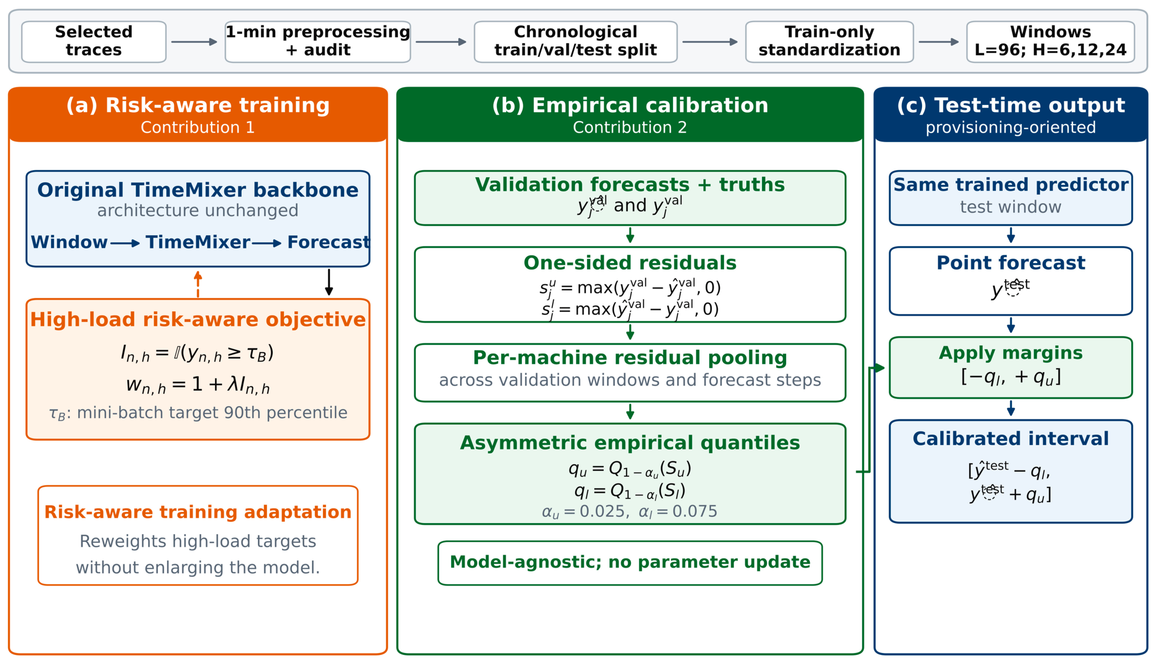
This section introduces the RA-TimeMixer framework. The objective is not to redesign the TimeMixer forecasting backbone, but to adapt it to the high-load underestimation risk that arises in cloud CPU provisioning. RA-TimeMixer consists of three parts: a TimeMixer point forecasting backbone, a high-load risk-aware loss during training, and a post hoc asymmetric upper-bound calibration procedure. The overall framework is shown in Figure 1.

3.1. Problem Definition

This work studies univariate multi-step forecasting of machine-level cloud CPU utilization. For machine $i$, its regularized one-minute CPU utilization sequence obtained after minute-level aggregation and explicit missingness handling is denoted as follows:

$${\mathbf{x}}^{\left(i\right)}=\left(x_1^{\left(i\right)},x_2^{\left(i\right)},\dots ,x_{T_i}^{\left(i\right)}\right),$$

(1)

where $x_t^{\left(i\right)}$ is the CPU utilization of machine $i$ at time step $t$ and $T_i$ is the length of the machine sequence. Given an input length $L$, the historical input window at time step $t$ is

$$\mathbf{X}{t}^{\left(i\right)}=\left(x{t-L+1}^{\left(i\right)},x_{t-L+2}^{\left(i\right)},\dots ,x_t^{\left(i\right)}\right),$$

(2)

and the future $H$-step forecasting target is

$$\mathbf{Y}{t}^{\left(i\right)}=\left(x{t+1}^{\left(i\right)},x_{t+2}^{\left(i\right)},\dots ,x_{t+H}^{\left(i\right)}\right).$$

(3)

The machine-level multi-step CPU utilization forecasting model can therefore be written as

$${\stackrel{\mathbf{ˆ}}{\mathbf{Y}}}_t^{\left(i\right)}=f_{\theta }\left({\mathbf{X}}_t^{\left(i\right)}\right),$$

(4)

where $f_{\theta }$ is the forecasting model with parameters $\theta$ and ${\stackrel{\mathbf{ˆ}}{\mathbf{Y}}}_t^{\left(i\right)}$ is the $H-step$ point forecast. In the experiments, $L=96$ and $H \in \{6, 12, 24\}$. Since the sampling interval is 1 min, these horizons correspond to forecasts for the next 6, 12, and 24 min.

3.2. RA-TimeMixer Framework

RA-TimeMixer is a provisioning-oriented adaptation of Original TimeMixer. Original TimeMixer uses multiscale temporal mixing to model patterns at different sampling scales and generate multi-step forecasts [13]. This paper keeps that backbone unchanged and adds risk-oriented extensions at the training-objective and post hoc calibration stages.

The pipeline has three stages. First, candidate machines are selected by valid raw-record counts, their observations are aggregated to one-minute bins, missingness is audited before regularization, the sequences are reindexed and interpolated where necessary, and chronological training, validation, and test segments are converted into sliding windows. Second, the TimeMixer backbone maps each input window to a multi-step point forecast. Original TimeMixer is trained with the standard point-prediction loss, whereas RA-TimeMixer is trained with a high-load risk-aware loss. Third, pooled validation residuals are used to construct calibrated upper bounds for test predictions. The calibration module is post hoc and does not update model parameters.

The two RA-TimeMixer extensions play different roles. The high-load risk-aware loss is a training objective that influences parameter updates; asymmetric upper-bound calibration is a post hoc calibration module that uses validation residuals after model training. Thus, RA-TimeMixer preserves the TimeMixer multiscale architecture while aligning its output with the risk structure of cloud CPU provisioning.

3.3. High-Load Risk-Aware Loss

A standard MSE loss weights all samples equally and therefore mainly optimizes global average error. In cloud CPU forecasting, this objective may not adequately reflect the potentially different consequences of prediction errors during high-load periods. RA-TimeMixer therefore uses a batch-wise high-load weighted MSE loss.

For each mini-batch, all true target values across samples and forecast steps are collected as

$$B=\left\{y_{n,h}\mid n=1,\dots ,N;h=1,\dots ,H\right\},$$

(5)

where $N$ is the mini-batch size and $H$ is the prediction length. The batch-wise high-load cutoff is defined as the $q$-quantile of these target values:

$${\tau }_B=Q_q\left(B\right).$$

(6)

In Equation (6), $q$ denotes the mini-batch target quantile; the default setting is $q=0.90$.

For the $n-th$ sample and $h-th$ forecast step, the high-load indicator is

$$I_{n,h}=\mathbb{I}\left(y_{n,h}\ge {\tau }_B\right),$$

(7)

where $\mathbb{I}\left(\cdot \right)$ is the indicator function. The high-load risk-aware loss is then

$${\mathcal{L}}_{\mathrm{R}\mathrm{A}}={\displaystyle \frac{1}{NH}}{\displaystyle \sum _{n=1}^N}{\displaystyle \sum _{h=1}^H}\left(1+\lambda I_{n,h}\right){\left({\hat{y}}_{n,h}-y_{n,h}\right)}^2,$$

(8)

In Equation (8), $\lambda$ is the additional weight assigned to high-load target points. Target points below the batch-wise high-load cutoff receive the ordinary MSE weight, whereas target points at or above the cutoff receive the additional squared-error weight. This design shifts part of the training objective toward high-load prediction behavior. The mini-batch quantile used for training is distinct from the retrospective test-derived and training-derived thresholds used only for evaluation.

The final implementation uses high-load weighting rather than directional underestimation penalization. No additional asymmetric penalty is applied to underestimated samples. The term high-load risk-aware loss is used because the loss gives larger weight to high-load targets, not because overestimation and underestimation errors receive different directional costs. The expected outcome is therefore not necessarily a lower global MSE, but a provisioning-oriented trade-off: a modest average-error cost may be accepted if high-load underestimation metrics improve. The default setting $q=0.90$ and $\lambda =0.50$ is treated as a moderate accuracy–risk operating point rather than as an optimal hyperparameter configuration; its sensitivity is examined in Section 5.6.3.

3.4. Asymmetric Upper-Bound Calibration

Beyond point forecasts, cloud provisioning often requires a conservative upper estimate of future utilization. After model training, RA-TimeMixer applies post hoc asymmetric upper-bound calibration. Let ${\hat{\mathrm{y}}}_j$ and $y_j$ denote the point forecast and true value for calibration sample $j$. Symmetric calibration uses absolute residual scores:

$$s_j^{\mathrm{s}\mathrm{y}\mathrm{m}}=\left|y_j-{\hat{y}}_j\right|.$$

(9)

Given a target failure rate $\alpha$, symmetric calibration computes a common margin $q_{\mathrm{s}\mathrm{y}\mathrm{m}}$ as the finite-sample-adjusted higher empirical quantile of the pooled absolute validation residuals, using Equation (13) with $\beta =1-\alpha$, and constructs the test interval

$$L_j={\hat{\mathrm{y}}}_j-q_{\mathrm{s}\mathrm{y}\mathrm{m}}, U_j={\hat{\mathrm{y}}}_j+q_{\mathrm{s}\mathrm{y}\mathrm{m}}.$$

(10)

Because provisioning mainly concerns whether the realized load exceeds the upper bound, this work separates one-sided residual scores:

$$s_j^u=max\left(y_j-{\hat{\mathrm{y}}}_j,0\right),s_j^l=max\left({\hat{\mathrm{y}}}_j-y_j,0\right).$$

(11)

The total target failure rate $\alpha$ is split asymmetrically between the upper and lower sides. Let ${\alpha }_u$ and ${\alpha }_l$ denote the upper-side and lower-side failure rates:

$${\alpha }_u=\rho \alpha ,{\alpha }_l=\left(1-\rho \right)\alpha ,{\alpha }_u+{\alpha }_l=\alpha .$$

(12)

In the experiments, $\alpha =0.10$ and $\rho =0.25$, so the upper side receives ${\alpha }_u=0.025$ and the lower side receives ${\alpha }_l=0.075$. The pooled one-sided residual score sets and their calibration quantiles are

$$S_u={\left\{s_j^u\right\}}_{j=1}^M,S_l={\left\{s_j^l\right\}}_{j=1}^M,q_u=Q_{1-{\alpha }_u}\left(S_u\right),q_l=Q_{1-{\alpha }_l}\left(S_l\right).$$

(13)

In Equation (13), $M$ denotes the number of pooled validation residual scores for the corresponding machine. For a score set of size $M$, $Q_{\beta }$ denotes the higher empirical quantile evaluated at level $min\{\lceil (M+1)\beta \rceil /M,1\}$, matching the implementation.

For a test point forecast, the asymmetric interval is

$$L_j={\hat{\mathrm{y}}}_j-q_l, U_j={\hat{\mathrm{y}}}_j+q_u,$$

(14)

In Equation (14), $U_j$ is the calibrated upper bound of interest. An upper-bound violation is recorded whenever the true test value exceeds this upper bound. The residual quantiles are estimated separately for each machine by pooling that machine’s validation residuals across all retained validation windows and forecast steps; residuals are not pooled across machines, and a separate margin is not estimated for each horizon. This design is simpler and more stable in the current 50-machine univariate forecasting setting.

This calibration should be interpreted as conformal-inspired empirical calibration in a limited sense: the upper-bound margin is obtained from empirical validation residual scores and residual quantiles. The procedure is not formal split conformal prediction. It does not assume exchangeability between validation and test residuals, does not provide distribution-free finite-sample coverage under temporal dependence or nonstationarity, and should be evaluated through chronological test-set metrics such as PICP, Upper violation rate, High-load upper violation rate, High-load provision under-magnitude, and Avg upper margin. The default upper-side allocation ratio of 0.25 is treated as a practical trade-off setting rather than as an optimum; sensitivity analyses are reported in Section 5.6.4 and Appendix A,

Table A9. Sensitivity to total target failure rate and upper-tail allocation.

Model	Alpha	Upper Ratio	PICP	MPIW	Upper Viol.	HL Upper Viol.	HL Under-Mag.	Upper Margin
Original	0.05	0.10	0.9413	3.0263	0.0077	0.0637	0.0376	2.1640
Original	0.05	0.25	0.9435	2.6385	0.0148	0.1112	0.0694	1.7230
Original	0.05	0.50	0.9457	2.4151	0.0277	0.1805	0.1149	1.3858
Original	0.10	0.10	0.8778	2.5027	0.0123	0.0949	0.0592	1.8500
Original	0.10	0.25 *	0.8815	2.0938	0.0277	0.1805	0.1149	1.3858
Original	0.10	0.50	0.8889	1.8888	0.0534	0.2877	0.1902	1.0581
Original	0.15	0.10	0.8161	2.1556	0.0174	0.1263	0.0793	1.6284
Original	0.15	0.25	0.8204	1.7761	0.0408	0.2394	0.1549	1.1919
Original	0.15	0.50	0.8309	1.5829	0.0783	0.3622	0.2501	0.8750
RA	0.05	0.10	0.9425	3.0332	0.0077	0.0635	0.0375	2.1267
RA	0.05	0.25	0.9446	2.6474	0.0149	0.1105	0.0688	1.6854
RA	0.05	0.50	0.9462	2.4307	0.0279	0.1795	0.1138	1.3523
RA	0.10	0.10	0.8791	2.5026	0.0124	0.0948	0.0588	1.8115
RA	0.10	0.25 *	0.8828	2.1000	0.0279	0.1795	0.1138	1.3523
RA	0.10	0.50	0.8900	1.8994	0.0538	0.2838	0.1886	1.0245
RA	0.15	0.10	0.8172	2.1543	0.0175	0.1254	0.0784	1.5930
RA	0.15	0.25	0.8213	1.7780	0.0411	0.2369	0.1536	1.1583
RA	0.15	0.50	0.8322	1.5908	0.0786	0.3566	0.2470	0.8431

Note: alpha denotes the total target failure rate; Upper ratio denotes the fraction assigned to the upper side. An asterisk marks the default setting used in Table 5. PICP, Upper viol., and HL upper viol. are proportions; MPIW, HL under-mag., and Upper margin are reported in the standardized evaluation space. Lower violation and under-magnitude values indicate fewer or less severe empirical upper-bound failures, whereas lower MPIW indicates narrower intervals.

.

Because the calibration margins are estimated from historical validation residuals, the current empirical procedure has limited extrapolation capability for unprecedented workload bursts that exceed the support of observed residuals. Under heavy-tailed cloud workload behavior, empirical residual quantiles may underestimate rare tail events if such events are absent from the validation segment. Future extensions could integrate Extreme Value Theory, for example, by fitting a Generalized Pareto Distribution to residual exceedances above a high threshold, to improve tail extrapolation beyond the observed validation residuals.

The present calibration is also static within the retrospective experiment. In an online resource orchestrator, the residual pool could be updated periodically with a sliding window of recent prediction errors, or with exponentially weighted residual updates that emphasize recent observations while retaining historical information. Such adaptive calibration may help the upper-bound margin respond to workload drift, but it requires separate online or closed-loop evaluation and is not claimed by the present retrospective study.

3.5. Training and Inference Procedure

The RA-TimeMixer workflow contains four stages: data preprocessing, model training, validation-set calibration, and test-set evaluation. During preprocessing, machine-level CPU records are aggregated to one-minute bins, missingness is audited before explicit regularization, and each machine is split chronologically into training, validation, and test segments. Standardization parameters are fitted only on training data and then applied to validation and test data, reducing leakage from future periods.

During training, sliding-window samples from the training segment are fed into the TimeMixer backbone. Original TimeMixer uses the standard point-prediction loss, whereas RA-TimeMixer uses the batch-wise high-load weighted MSE. The two models share the same backbone and main hyperparameters, so their comparison isolates the effect of the training objective rather than model capacity.

During validation calibration, the trained model generates validation forecasts and residual scores. Symmetric calibration estimates a pooled absolute residual margin; asymmetric calibration separately estimates pooled upper-side and lower-side residual margins. No model parameters are updated at this stage. During testing, point forecasts are used to compute MSE, MAE, and RMSE; high-load test regions are used to compute underestimation risk metrics; and calibrated intervals are used to compute upper-bound reliability metrics. This unified protocol allows the average-accuracy, high-load risk, and upper-bound reliability trade-offs to be analyzed together.

4. Experimental Setup

This section describes the dataset construction, preprocessing procedure, comparison models, evaluation metrics, and implementation details. The goal is not only to compare average point accuracy but also to evaluate high-load underestimation risk and upper-bound failure risk under the same machine-level CPU utilization forecasting task. All trainable models use the same Alibaba 2018 50-machine CPU subset, chronological split, input length, prediction lengths, standardization protocol, validation-based calibration, and test windows.

Unlike conventional forecasting experiments that report only MSE, MAE, and RMSE, the proposed provisioning-oriented evaluation protocol has three metric groups: conventional point forecast errors, high-load risk metrics, and upper-bound calibration metrics. Persistence reference comparisons, error-direction decomposition, raw-scale asymmetric-loss proxy diagnostics, and machine-level paired sign tests are also reported to assess whether results depend on a particular model class or on a small subset of machines.

4.1. Dataset and Preprocessing

Among 4023 machines containing valid CPU records, candidate machines were ranked in descending order according to their numbers of valid raw observations. A valid record required a numeric timestamp, a numeric CPU utilization value, and a CPU value within the range 0–100%. The first 50 machines were retained before model training or inspection of forecasting results. The retained machines contained between 64,026 and 65,044 valid raw observations. Forty-nine machines had record counts strictly above the selection cutoff of 64,026, while one machine was located exactly at the cutoff for the single remaining position; therefore, no count tie crossed the top-50 selection boundary. Timestamp continuity was audited after machine selection and was not used as a selection criterion.

After minute-level aggregation, missingness was audited before reindexing and imputation by comparing the observed timestamps of each machine with the complete one-minute grid between its first and last observed minutes. Across the 50 retained machines, 35,714 of 575,293 expected minute-level observations were missing, corresponding to an overall missing ratio of 6.208%. The median and maximum machine-level missing ratios were 6.328% and 6.754%, respectively, and the maximum interval between adjacent observed minute bins was 362 min. All missing values were internal grid points and were filled by linear interpolation; no boundary values required forward or backward filling. The resulting regularized sequences contained no remaining missing values. Detailed selection and missingness audits are reported in

Table A1. Data construction, machine-selection, and missingness audit.

(a) Machine-Selection Audit.
Audit Item	Value
Candidate machines with valid CPU records	4023
Ranking and selection rule	Descending valid raw-record count; first 50 retained
Selected machines/valid-record range	50/64,026–65,044
Cutoff structure	49 above and 1 at 64,026; no boundary tie
Minimum resampled length/machines passing	1000 points/50 of 50
Timestamp continuity used for selection	No
(b) Pre-Imputation Minute-Level Missingness Audit.
Audit Item	Value
Machines with missing minutes	50 of 50
Observed/expected minute bins	539,579/575,293
Missing bins/overall ratio	35,714/6.208%
Median/maximum machine missing ratio	6.328%/6.754%
Maximum pre-imputation gap	362 min
Gaps >1 min/>2 min	3115/1329
Internal interpolation/boundary filling	35,714/0 points
Remaining missing values after regularization	0

Note: Machine selection was completed before model training or inspection of forecasting results. No valid-record-count tie crossed the top-50 boundary, and timestamp continuity was not a selection criterion. Missingness was measured before one-minute reindexing and interpolation.

.

Each selected machine is represented as a separate univariate time series with cpu_util_percent as the forecasting target. The regularized sequence is split chronologically: the first 70% is used for training, the next 10% for validation and calibration, and the final 20% for testing. Standardization parameters are fitted on the training segment only and applied to the corresponding validation and test segments. The input window length is 96, and prediction lengths are 6, 12, and 24. Prediction length 12 is the main setting, while prediction lengths 6 and 24 are used for horizon-sensitivity analysis.

To assess whether the comparison depended on imputed observations, Original TimeMixer and RA-TimeMixer were additionally retrained and evaluated at prediction length 12 using only fully observed input-target windows containing 108 one-minute observations (96 input points and 12 forecast targets). Standardization parameters and machine-specific high-load thresholds were re-estimated from fully observed training values under this restricted protocol; the results are presented in Section 5.6.5.

4.2. Comparison Models

The trainable comparison models cover linear forecasting, recurrent neural networks, patch-based Transformer-style forecasting, and multiscale time mixing. DLinear uses moving-average decomposition with kernel size 25 and separate seasonal and trend linear mappings. GRU uses one unidirectional recurrent layer with hidden size 16, effective recurrent dropout 0, and a linear hidden-size-16-to-H forecasting head, where H denotes the prediction length ($H=12$ in the main setting). The lightweight PatchTST-style baseline uses patch length 16, stride 8, 11 patches, $d_{model}=16$, two attention heads, one Transformer encoder layer, $d_{ff}=32$, dropout 0.1, and GELU activation. Original TimeMixer is the direct backbone baseline and the most important comparison for RA-TimeMixer.

RA-TimeMixer is not treated as a new backbone. It uses the same TimeMixer architecture and main hyperparameters as Original TimeMixer; the training-stage difference is the high-load risk-aware loss, and the post-training extension is asymmetric upper-bound calibration. This controlled comparison separates risk-oriented modifications from changes in model capacity. Architecture-specific configurations and the common experimental protocol are reported in

Table A2. Model configurations and common experimental protocol.

(a) Architecture-Specific Configurations.
Model	Key Architecture		Training Loss
DLinear	Moving-average decomposition (kernel 25); input length 96 and output length H; separate seasonal and trend linear mappings		MSE
GRU	One-layer unidirectional GRU; hidden size 16; effective recurrent dropout 0; a linear hidden-size-16-to-H forecasting head		MSE
Lightweight PatchTST-style	Patch length 16; stride 8; 11 patches; $dmodel=16$; 2 heads; 1 encoder layer; $dff=32$; dropout 0.1; GELU		MSE
Original TimeMixer	Moving-average decomposition (kernel 25); $dmodel=16$; $dff=32$; one Past-Decomposable-Mixing block; channel independence; one average-downsampling layer, window 2		MSE
RA-TimeMixer	Same backbone and architecture as Original TimeMixer		High-load weighted MSE ($q=0.90$; additional weight $\lambda =0.50$)
(b) Common Training and Evaluation Protocol.
Setting		Value
Optimizer		Adam
Learning-rate scheduler		OneCycleLR (warm-up fraction = 0.2)
Maximum learning rate		0.001
Batch size		16
Maximum epochs		3
Early-stopping patience		1
Main random seed		2021
Checkpoint		Lowest validation MSE
Evaluation hardware		CPU-only Windows environment
Test DataLoader shuffle		No

Note: The seed analysis uses 2021–2023 for Original TimeMixer and RA-TimeMixer at $H=12$. Lightweight PatchTST-style denotes the compact implementation evaluated here, not a full reproduction of the original architecture. H is the prediction length; $H=12$ is the main setting, and $H=6$ and $H=24$ are used for horizon sensitivity where applicable. Representative median machine-wise training times were 33.30 s for Original TimeMixer and 33.58 s for RA-TimeMixer under the reported CPU-only environment ($n=3$ runs per model).

.

Persistence is additionally reported as a nonparametric reference baseline. It repeats the last observed input value across all forecast steps and requires no training. Because short-term CPU utilization can be strongly persistent, Persistence is treated as a serious reference rather than as a weak baseline.

4.3. Evaluation Metrics

The evaluation protocol contains four components. First, MSE, MAE, and RMSE measure average point forecasting accuracy over all test samples. Second, high-load risk metrics evaluate prediction behavior on realized high-load subsets. For each machine, the main retrospective high-load subset is defined using the machine-specific 90th percentile of the evaluated test true values. This cutoff is used only to partition the realized test trajectory for evaluation; it is not available to the model during training, validation, calibration, or prediction. Alternative retrospective percentiles and a training-derived threshold are examined separately in the robustness analysis.

High-load MAE measures the mean absolute error over high-load samples. Under-rate high measures the proportion of high-load samples for which the forecast is below the true value. Under-magnitude high measures the mean nonnegative underestimation amount over high-load samples. Under-MAE when under measures the conditional severity after high-load underestimation occurs. These retrospective metrics are empirical forecasting-level proxies for potential under-provisioning risk and should not be interpreted as direct measurements of service-level violations, latency, resource cost, or online scaling outcomes.

Third, upper-bound calibration metrics evaluate empirical reliability of calibrated intervals and upper bounds. PICP measures interval coverage, MPIW measures average interval width, Upper violation rate measures the frequency with which the true value exceeds the predicted upper bound, High-load upper violation rate focuses on failures within realized high-load samples, High-load provision under-magnitude is the mean nonnegative exceedance $max\left(y-U,0\right)$ over all realized high-load samples, and Avg upper margin measures the average upper margin relative to the point forecast.

Fourth, machine-level robustness is assessed by paired win/loss statistics and two-sided exact sign tests. Each retained machine is treated as one paired observational unit. Lower metric values count as wins for RA-TimeMixer, equal values as ties, and higher values as losses. Exact tests are computed on non-tied machine pairs and are interpreted as evidence of directional consistency across the retained machines. Unless otherwise stated, MSE, MAE, RMSE, High-load MAE, Under-magnitude high, Under-MAE when under, MPIW, High-load provision under-magnitude, and Avg upper margin are computed in each machine’s standardized evaluation space; rate-based metrics are reported as proportions. 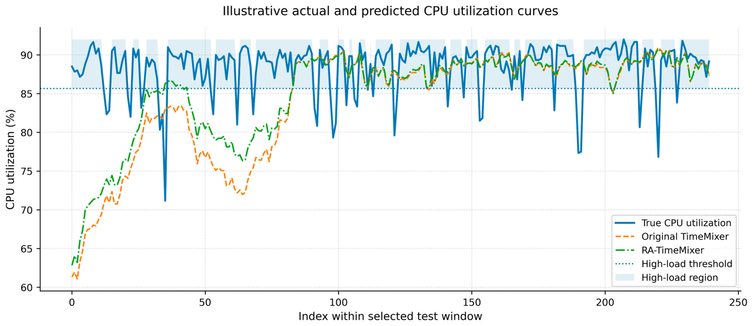Figure 2 is inverse-transformed to the original CPU utilization percentage scale for visualization.

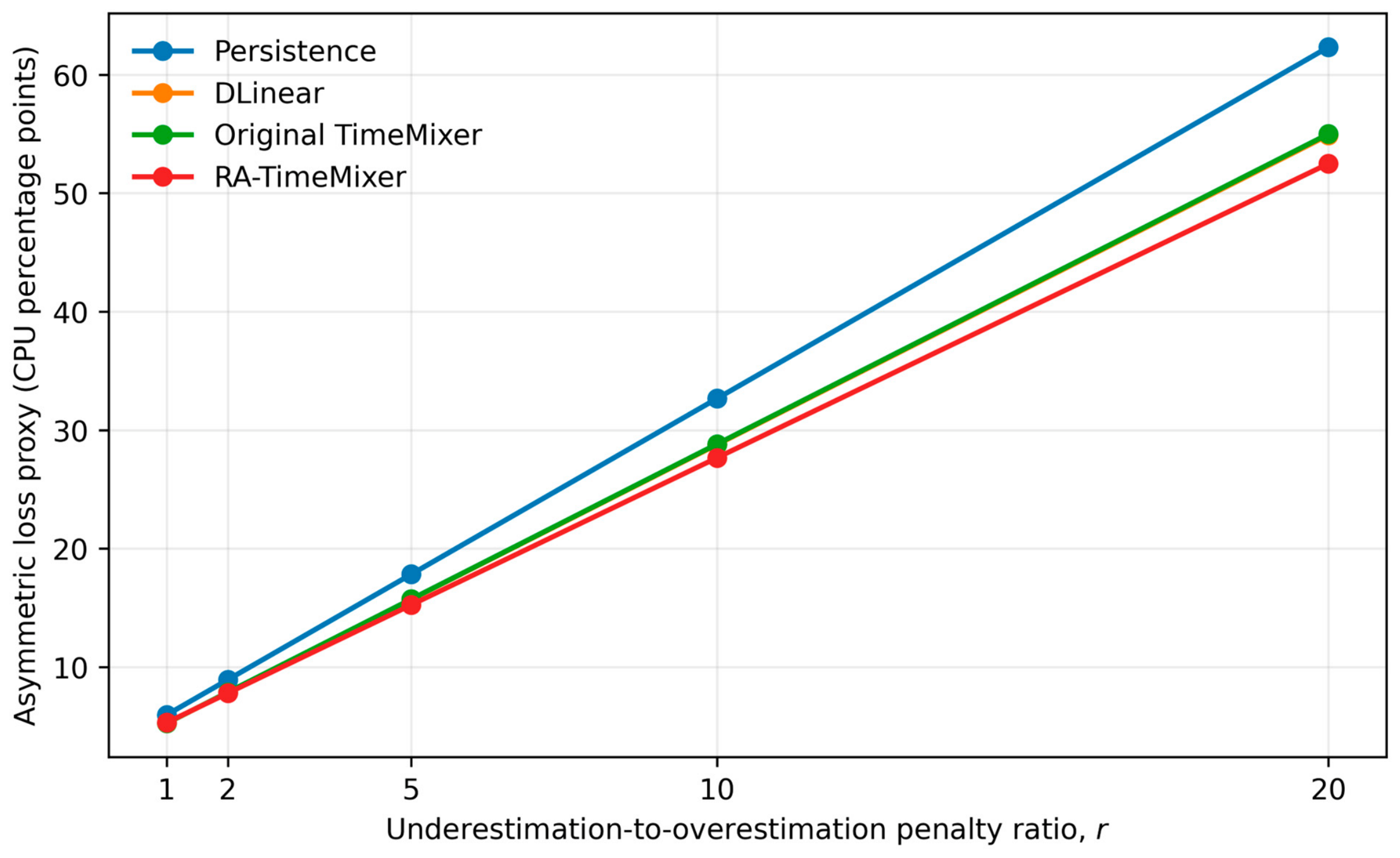
To examine why Persistence is competitive and whether the RA-TimeMixer risk reduction reflects a general upward forecast shift, the prediction-length-12 follow-up analysis decomposes raw-scale forecast error into signed bias, unconditional underestimation magnitude, and unconditional overestimation magnitude. It also reports a provisioning-oriented asymmetric-loss proxy, $C_r= r \mathrm{m}\mathrm{a}\mathrm{x}(y - a, 0) + \mathrm{m}\mathrm{a}\mathrm{x}(a - y, 0)$, for $r \in \{1,2,5,10,20\}$, where a is the forecast clipped to the valid 0–100% CPU range. These diagnostics are computed over all stored multi-step forecast elements separately for each machine and then macro-averaged across machines. They are empirical loss proxies rather than measurements of monetary cost, service-level violations, or scheduler outcomes. The follow-up high-load domain uses each machine’s 90th-percentile threshold estimated from its chronological training segment.

4.4. Implementation Details

All trainable models are evaluated under a fixed compact training budget. Each trainable model is trained, validated, and tested separately for each machine. They use Adam optimization with a OneCycleLR schedule with a warm-up fraction of 0.2, a maximum learning rate of 0.001, batch size 16, at most three epochs, and validation-loss early stopping with patience 1. The checkpoint with the lowest validation MSE is restored before test evaluation. The original training script also logs test loss after each epoch for diagnostic purposes, but the logged test loss is not part of the scripted optimization, early stopping, checkpoint selection, calibration, or model-ranking procedures. This protocol supports a controlled CPU-only comparison and is not presented as an exhaustive hyperparameter search.

Experiments are conducted in a CPU-only Windows environment without GPU acceleration or automatic mixed precision. Unless otherwise stated, the main experiments use random seed 2021, with Python, NumPy, and PyTorch seeds fixed consistently. The three-seed analysis uses seeds 2021, 2022, and 2023 for Original TimeMixer and RA-TimeMixer at prediction length 12. Training, validation, and test segments are chronological. Training and validation DataLoaders are shuffled, whereas the test DataLoader is not. All use drop_last = True, retaining only complete batches. The software environment includes Python 3.13.2, PyTorch 2.12.0+cpu, NumPy 2.3.5, pandas 2.3.3, scikit-learn 1.7.2, SciPy 1.17.0, and matplotlib 3.10.8.

Original TimeMixer and RA-TimeMixer share moving-average decomposition with kernel size 25, $d_{model}=16$, $d_{ff}=32$, one Past-Decomposable-Mixing block ($e_{layers}=1$), channel independence, and one average-downsampling layer with window size 2. RA-TimeMixer uses $q=0.90$, an additional high-load weight of 0.50, and no directional underestimation penalty. Asymmetric calibration uses a total target failure rate of 0.10 and an upper-side allocation ratio of 0.25, yielding upper- and lower-side target failure rates of 0.025 and 0.075. Full model configurations are given in Table A2.

Training-log auditing of the 50 Original TimeMixer runs and 50 RA-TimeMixer runs showed median signed relative changes between the penultimate and final recorded validation losses of 0.0088% and 0.0732%, respectively. The audit defines the signed relative change as the final-minus-penultimate validation-loss difference divided by the absolute penultimate loss; positive values indicate an increase and negative values a decrease. Six Original TimeMixer runs and eleven RA-TimeMixer runs recorded two epochs, whereas the remaining runs recorded three epochs. Separately, source-code auditing confirmed that the checkpoint with the lowest validation loss was restored before validation and test prediction generation. The near-zero median changes indicate limited median variation near the end of the recorded training trajectories under the maximum-three-epoch protocol, but they do not establish formal convergence. The main results are reported as unweighted averages of machine-level metrics.

5. Results and Discussion

This section reports the empirical results on the Alibaba 2018 machine-level CPU utilization subset. The analysis focuses on whether RA-TimeMixer can reduce high-load underestimation risk and empirical upper-bound violation risk while maintaining comparable point forecasting accuracy. The goal is not to show that RA-TimeMixer is the best model on all average point-error metrics, but to examine the trade-off induced by high-load risk-aware training and asymmetric upper-bound calibration.

5.1. Conventional Point Forecasting Accuracy

Table 1. Main point forecasting accuracy at prediction length 12.

Trainable-Model Rank	Model	MSE	MAE	RMSE
1	DLinear	0.3719	0.4525	0.6064
2	Original TimeMixer	0.3757	0.4528	0.6091
3	RA-TimeMixer	0.3783	0.4579	0.6113
4	GRU	0.4399	0.4850	0.6519
5	Lightweight PatchTST-style	0.4545	0.4911	0.6610

Note: MSE, MAE, and RMSE denote mean squared error, mean absolute error, and root mean squared error, respectively. The rank column includes trainable models only; lower values indicate better point accuracy.

reports conventional point forecasting errors at prediction length 12. These metrics evaluate average prediction accuracy over all test samples.

DLinear obtains the lowest average point-error values, with MSE, MAE, and RMSE of 0.3719, 0.4525, and 0.6064, respectively. Original TimeMixer is close to DLinear, while RA-TimeMixer has slightly larger point errors than both DLinear and Original TimeMixer but remains better than GRU and the lightweight PatchTST-style baseline. This result indicates that RA-TimeMixer is not the best average-error model. The small degradation relative to Original TimeMixer is consistent with the training objective, which assigns additional weight to high-load samples rather than optimizing global average error alone.

At the same time, RA-TimeMixer remains close to Original TimeMixer on point accuracy. Thus, the high-load risk-aware loss does not substantially damage the overall forecasting capability of the TimeMixer backbone. Table 1 should therefore be interpreted as evidence of a limited average-accuracy cost that creates room for risk reduction in high-load regions.

Figure 2 is a deterministically selected qualitative illustration and is not used as independent ranking evidence; the quantitative comparison relies on Table 2, Table 3 and Table 4 and the machine-level statistics in Appendix A.

5.2. High-Load Risk Metrics

Table 2 reports provisioning-oriented high-load risk metrics at prediction length 12. These metrics evaluate prediction errors and underestimation within the realized high-load subset of the test targets.

Table 2. Main high-load risk metrics at prediction length 12.

Trainable-Model Rank	Model	High-Load MAE	Under-Rate High	Under-Magnitude High	Under-MAE When Under
1	RA-TimeMixer	0.7853	0.8234	0.7277	0.8877
2	Original TimeMixer	0.8073	0.8393	0.7585	0.9056
3	DLinear	0.8413	0.8808	0.8060	0.9188
4	GRU	1.0591	0.9133	1.0405	1.1221
5	Lightweight PatchTST-style	1.0775	0.8904	1.0484	1.1529

Note: Rank is based on High-load MAE among the trainable models; Persistence is reported separately in

Table A3. Persistence reference baseline and machine-level paired robustness.

(a) Persistence Baseline Under the Main Retrospective High-Load Definition.
Pred. Len	MSE	MAE	RMSE	HL-MAE	Under-Rate	Under-Mag.	Under-MAE
6	0.4080	0.4577	0.6340	0.6417	0.6872	0.5403	0.7706
12	0.5041	0.5147	0.7055	0.7595	0.7195	0.6500	0.8897
24	0.6100	0.5713	0.7767	0.8788	0.7463	0.7628	1.0134
(b) Core Machine-Level Paired Exact Sign Test Results.
h	Comparison		Metric	Win/Tie/Loss	Non-Tied N		Exact p
12	RA vs. Original		HL-MAE	44/0/6	50		<0.001
12	RA vs. Original		Under-mag.	44/0/6	50		<0.001
12	RA vs. DLinear		HL-MAE	47/0/3	50		<0.001
12	RA vs. DLinear		Under-mag.	48/0/2	50		<0.001
24	RA vs. Original		HL-MAE	49/0/1	50		<0.001
24	RA vs. Original		Under-mag.	48/0/2	50		<0.001

Note: HL-MAE denotes High-load MAE; Under-mag. denotes Under-magnitude high. Win/Tie/Loss is ordered from the RA-TimeMixer perspective. Two-sided exact sign tests use non-tied machine pairs. Error-magnitude metrics are reported in the standardized evaluation space.

(a). Lower values indicate better performance on the retrospective high-load metrics.

Table 2. Main high-load risk metrics at prediction length 12.

Trainable-Model Rank	Model	High-Load MAE	Under-Rate High	Under-Magnitude High	Under-MAE When Under
1	RA-TimeMixer	0.7853	0.8234	0.7277	0.8877
2	Original TimeMixer	0.8073	0.8393	0.7585	0.9056
3	DLinear	0.8413	0.8808	0.8060	0.9188
4	GRU	1.0591	0.9133	1.0405	1.1221
5	Lightweight PatchTST-style	1.0775	0.8904	1.0484	1.1529

Note: Rank is based on High-load MAE among the trainable models; Persistence is reported separately in Table A3(a). Lower values indicate better performance on the retrospective high-load metrics.

RA-TimeMixer achieves the lowest value among the trainable models on all four high-load risk metrics. Relative to Original TimeMixer, it reduces High-load MAE by approximately 2.72%, Under-rate high by 1.89%, Under-magnitude high by 4.06%, and Under-MAE when under by 1.98%. The largest relative improvement is observed for Under-magnitude high, which is particularly relevant as a forecasting-level proxy for potential under-provisioning severity because it measures how much the model underestimates realized high-load utilization.

The improvement in Under-rate high is smaller, but its direction is consistent with the method design. RA-TimeMixer reduces both the frequency and the magnitude of high-load underestimation relative to Original TimeMixer and DLinear. The conditional Under-MAE when under also improves, indicating lower error severity after high-load underestimation occurs.

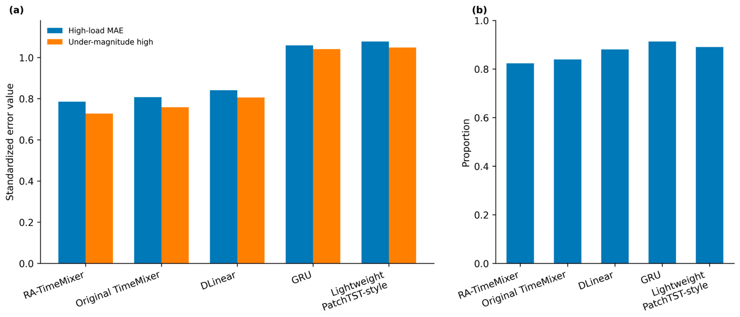
Figure 3 visualizes the main risk metrics. RA-TimeMixer consistently shows lower high-load risk values than Original TimeMixer and the other trainable baselines. This supports the interpretation that the high-load risk-aware loss shifts part of the TimeMixer optimization behavior from average-error minimization toward lower retrospective high-load underestimation metrics.

5.3. Ablation of the High-Load Risk-Aware Loss

Table 3 isolates the effect of the high-load risk-aware loss by comparing Original TimeMixer and RA-TimeMixer under the same backbone setting. Unlike the calibration comparison in Table 5, this ablation focuses on the training-stage loss design.

Table 3. Ablation study of the high-load risk-aware loss.

Variant	Loss	MSE	MAE	RMSE	HL-MAE	Under-Rate	Under-Mag.	Under-MAE
Original TimeMixer	MSE	0.3757	0.4528	0.6091	0.8073	0.8393	0.7585	0.9056
RA-TimeMixer	High-load risk-aware loss	0.3783	0.4579	0.6113	0.7853	0.8234	0.7277	0.8877

Note: HL-MAE denotes High-load MAE; Under-mag. denotes Under-magnitude high; Under-MAE denotes Under-MAE when under. Lower values indicate better performance.

Table 3. Ablation study of the high-load risk-aware loss.

Variant	Loss	MSE	MAE	RMSE	HL-MAE	Under-Rate	Under-Mag.	Under-MAE
Original TimeMixer	MSE	0.3757	0.4528	0.6091	0.8073	0.8393	0.7585	0.9056
RA-TimeMixer	High-load risk-aware loss	0.3783	0.4579	0.6113	0.7853	0.8234	0.7277	0.8877

Note: HL-MAE denotes High-load MAE; Under-mag. denotes Under-magnitude high; Under-MAE denotes Under-MAE when under. Lower values indicate better performance.

RA-TimeMixer has slightly larger conventional point errors than Original TimeMixer, confirming that the high-load risk-aware loss does not primarily optimize global average error. However, RA-TimeMixer improves all high-load risk metrics: High-load MAE decreases from 0.8073 to 0.7853, Under-rate high from 0.8393 to 0.8234, Under-magnitude high from 0.7585 to 0.7277, and Under-MAE when under from 0.9056 to 0.8877.

This ablation is central to the method claim. Since the backbone and main hyperparameters are the same, the improvement in high-load risk metrics is not attributable to increased model capacity or a different architecture; it is attributable to the high-load risk-aware training objective.

5.4. Horizon Sensitivity

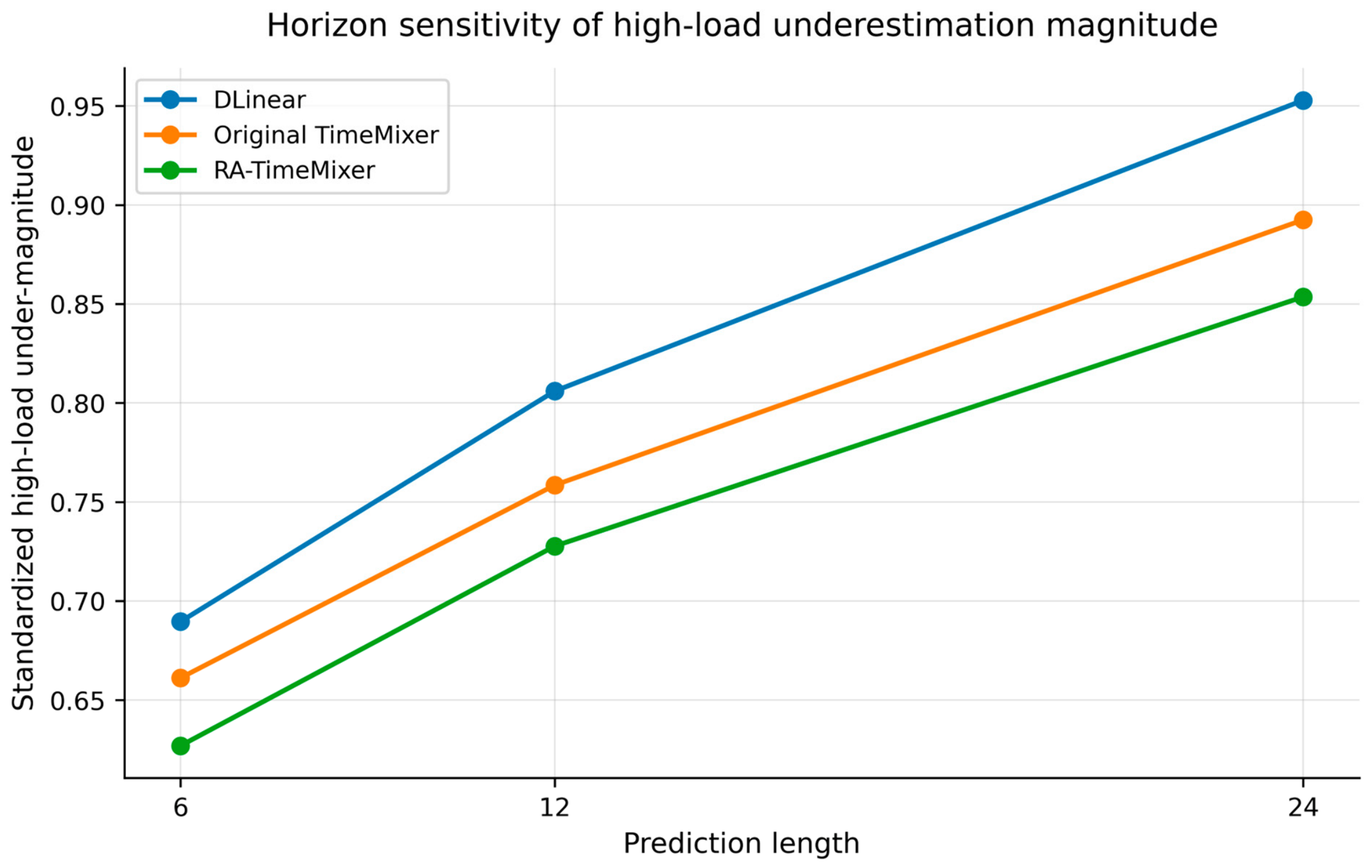
Table 4 compares DLinear, Original TimeMixer, and RA-TimeMixer across prediction lengths 6, 12, and 24, while Figure 4 visualizes Under-magnitude high across horizons.

Table 4. Horizon sensitivity of high-load risk metrics under prediction lengths 6, 12, and 24.

Pred. Len	Model	HL-MAE	Under-Rate	Under-Mag.	Under-MAE
6	DLinear	0.7282	0.8609	0.6896	0.8038
6	Original TimeMixer	0.7082	0.8308	0.6612	0.7990
6	RA-TimeMixer	0.6822	0.8092	0.6270	0.7785
12	DLinear	0.8413	0.8808	0.8060	0.9188
12	Original TimeMixer	0.8073	0.8393	0.7585	0.9056
12	RA-TimeMixer	0.7853	0.8234	0.7277	0.8877
24	DLinear	0.9802	0.9087	0.9529	1.0493
24	Original TimeMixer	0.9363	0.8601	0.8925	1.0378
24	RA-TimeMixer	0.9080	0.8409	0.8536	1.0153

Note: HL-MAE denotes High-load MAE; Under-mag. denotes Under-magnitude high; Under-MAE denotes Under-MAE when under. Lower values indicate smaller retrospective high-load errors and underestimation.

Table 4. Horizon sensitivity of high-load risk metrics under prediction lengths 6, 12, and 24.

Pred. Len	Model	HL-MAE	Under-Rate	Under-Mag.	Under-MAE
6	DLinear	0.7282	0.8609	0.6896	0.8038
6	Original TimeMixer	0.7082	0.8308	0.6612	0.7990
6	RA-TimeMixer	0.6822	0.8092	0.6270	0.7785
12	DLinear	0.8413	0.8808	0.8060	0.9188
12	Original TimeMixer	0.8073	0.8393	0.7585	0.9056
12	RA-TimeMixer	0.7853	0.8234	0.7277	0.8877
24	DLinear	0.9802	0.9087	0.9529	1.0493
24	Original TimeMixer	0.9363	0.8601	0.8925	1.0378
24	RA-TimeMixer	0.9080	0.8409	0.8536	1.0153

Note: HL-MAE denotes High-load MAE; Under-mag. denotes Under-magnitude high; Under-MAE denotes Under-MAE when under. Lower values indicate smaller retrospective high-load errors and underestimation.

As prediction length increases from 6 to 24, all models show higher high-load risk metrics, reflecting the increased uncertainty of longer-horizon forecasting. Across all three horizons, RA-TimeMixer keeps lower High-load MAE and Under-magnitude high than Original TimeMixer. Relative to Original TimeMixer, the reductions in Under-magnitude high are approximately 5.17%, 4.06%, and 4.36% at horizons 6, 12, and 24, respectively.

Figure 4 shows that RA-TimeMixer remains below Original TimeMixer and DLinear for Under-magnitude high at all horizons. The advantage is therefore not confined to a single prediction length. Combined with Table 1 and Table 3, these results show that RA-TimeMixer is designed for risk reduction rather than average point-error dominance.

5.5. Empirical Results of Asymmetric Upper-Bound Calibration

Table 5 compares pooled symmetric calibration and pooled residual-based asymmetric upper-bound calibration for Original TimeMixer and RA-TimeMixer. This experiment evaluates the post hoc calibration module, whereas Table 3 evaluates the training-stage loss. Within each machine, residual scores are pooled across all retained validation windows and forecast steps.

Table 5. Machine-wise pooled upper-bound calibration comparison on the 50-machine Alibaba subset. Symmetric and asymmetric calibration are applied separately to each machine using residuals pooled across that machine’s retained validation windows and forecast steps. The asymmetric setting assigns a smaller target failure rate to the upper side to reduce empirical upper-bound violation risk.

Variant	RA Loss	Asym. Cal.	PICP	MPIW	Upper Viol.	HL Upper Viol.	HL Under-Mag.	Upper Margin
Original + sym.	No	No	0.8938	1.8724	0.0692	0.3368	0.2293	0.9362
Original + asym.	No	Yes	0.8815	2.0938	0.0277	0.1805	0.1149	1.3858
RA + sym.	Yes	No	0.8933	1.8823	0.0642	0.3165	0.2146	0.9411
RA + asym.	Yes	Yes	0.8828	2.1000	0.0279	0.1795	0.1138	1.3523

Note: PICP denotes prediction interval coverage probability; MPIW denotes mean prediction interval width; HL denotes high-load; Upper viol. denotes Upper violation rate; HL upper viol. denotes High-load upper violation rate; HL under-mag. denotes High-load provision under-magnitude; sym. denotes symmetric calibration; asym. denotes asymmetric calibration. PICP, Upper viol., and HL upper viol. are proportions, whereas MPIW, HL under-mag., and Upper margin are reported in the standardized evaluation space.

Table 5. Machine-wise pooled upper-bound calibration comparison on the 50-machine Alibaba subset. Symmetric and asymmetric calibration are applied separately to each machine using residuals pooled across that machine’s retained validation windows and forecast steps. The asymmetric setting assigns a smaller target failure rate to the upper side to reduce empirical upper-bound violation risk.

Variant	RA Loss	Asym. Cal.	PICP	MPIW	Upper Viol.	HL Upper Viol.	HL Under-Mag.	Upper Margin
Original + sym.	No	No	0.8938	1.8724	0.0692	0.3368	0.2293	0.9362
Original + asym.	No	Yes	0.8815	2.0938	0.0277	0.1805	0.1149	1.3858
RA + sym.	Yes	No	0.8933	1.8823	0.0642	0.3165	0.2146	0.9411
RA + asym.	Yes	Yes	0.8828	2.1000	0.0279	0.1795	0.1138	1.3523

Note: PICP denotes prediction interval coverage probability; MPIW denotes mean prediction interval width; HL denotes high-load; Upper viol. denotes Upper violation rate; HL upper viol. denotes High-load upper violation rate; HL under-mag. denotes High-load provision under-magnitude; sym. denotes symmetric calibration; asym. denotes asymmetric calibration. PICP, Upper viol., and HL upper viol. are proportions, whereas MPIW, HL under-mag., and Upper margin are reported in the standardized evaluation space.

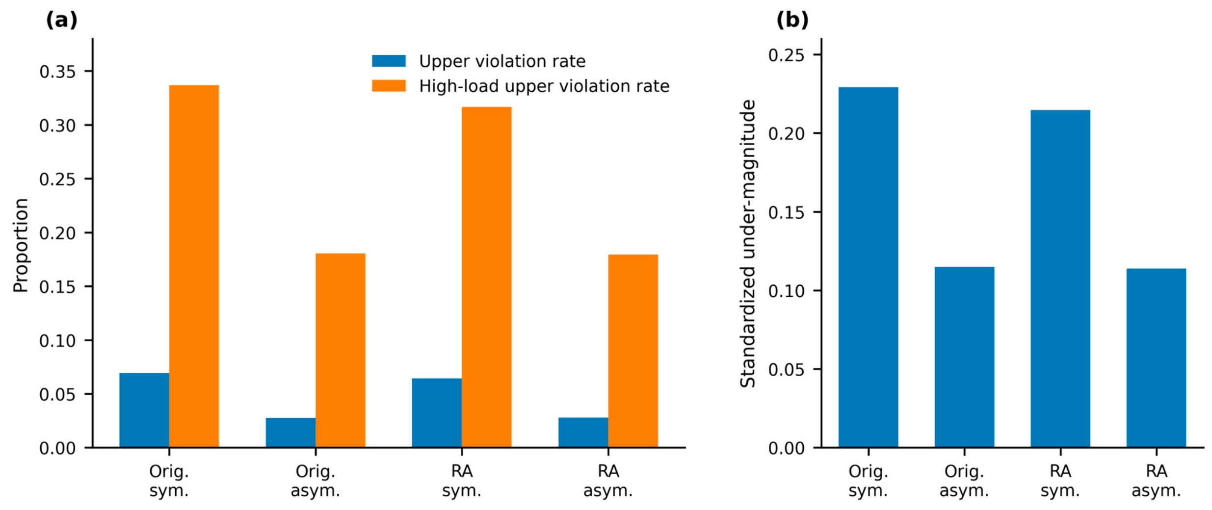
Asymmetric upper-bound calibration substantially lowers both overall and high-load upper-bound violation rates. For Original TimeMixer, Upper violation rate decreases from 0.0692 to 0.0277 and High-load upper violation rate from 0.3368 to 0.1805. For RA-TimeMixer, Upper violation rate decreases from 0.0642 to 0.0279 and High-load upper violation rate from 0.3165 to 0.1795. High-load provision under-magnitude is also reduced for both backbones. Figure 5 visualizes the corresponding upper-bound violation and high-load upper-bound risk metrics under symmetric and asymmetric calibration.

The calibration improvement has a cost. Asymmetric calibration increases MPIW and Avg upper margin relative to symmetric calibration, and PICP changes slightly. Thus, the asymmetric procedure should be interpreted as a provisioning-oriented empirical calibration trade-off: it uses wider intervals and more conservative upper margins to reduce the observed frequency and severity of upper-bound failures, especially within realized high-load subsets.

Taken together, the high-load risk-aware loss and asymmetric upper-bound calibration act on different stages. The loss modifies model training and primarily affects high-load point forecast behavior; the calibration module modifies prediction outputs after training and primarily affects upper-bound reliability. RA-TimeMixer therefore consists of coordinated risk-oriented training, calibration, and evaluation rather than a single loss-term modification.

5.6. Robustness and Sensitivity Analyses

5.6.1. Persistence and Machine-Level Robustness

Persistence is included as a reference baseline because short-term CPU utilization exhibits strong temporal persistence. Under the same retrospective 90th-percentile evaluation used in the main risk analysis, Table A3(a) shows that Persistence is competitive on several high-load metrics. At prediction length 12, its High-load MAE, Under-rate high, and Under-magnitude high are 0.7595, 0.7195, and 0.6500, respectively, below the corresponding RA-TimeMixer values; its Under-MAE when under is 0.8897, slightly above RA-TimeMixer. However, its MSE, MAE, and RMSE are 0.5041, 0.5147, and 0.7055, all clearly worse than RA-TimeMixer. Persistence is therefore a strong short-horizon state-continuation reference, but it does not dominate the overall accuracy–risk profile.

Machine-level paired results in Table A3(b) show that RA-TimeMixer improves High-load MAE and Under-magnitude high over Original TimeMixer on 44 of 50 machines at prediction length 12 and on 49 and 48 machines, respectively, at prediction length 24. The corresponding exact sign tests yield p < 0.001. These tests support directional consistency across the retained machines rather than population-level independence across the cluster.

5.6.2. Threshold-Definition Robustness

Table A4. Robustness to alternative high-load threshold definitions.

(a) Retrospective Evaluation Thresholds Based on Realized Test Values.
Threshold	HL-MAE Impr.	Under-Rate Impr.	Under-Mag. Impr.	Under-MAE Impr.	Under-Mag. W/T/L
80th pct.	2.2205%	2.3198%	4.2347%	1.8326%	44/0/6
85th pct.	2.4270%	2.1261%	4.1364%	1.8804%	44/0/6
90th pct.	2.7192%	1.8941%	4.0624%	1.9779%	44/0/6
95th pct.	3.1305%	1.9349%	4.0943%	1.8291%	42/0/8
(b) Training-Derived Machine-Specific 90th-Percentile Threshold.
Model		HL-MAE	Under-Rate High	Under-Mag.	Under-MAE
DLinear		0.915876	0.886477	0.884928	0.997437
GRU		1.057379	0.944088	1.047966	1.108347
Lightweight PatchTST-style		1.063716	0.916422	1.044890	1.136097
Original TimeMixer		0.877464	0.840914	0.832351	0.982333
RA-TimeMixer		0.852126	0.821454	0.797797	0.965617

Note: Panel (a) changes only the retrospective evaluation cutoff; models are not retrained or recalibrated. Positive improvement values indicate lower RA-TimeMixer metrics than Original TimeMixer. Panel (b) defines high load using each machine’s training segment, providing a deployment-compatible threshold analysis. Lower values indicate better performance.

(a) varies the retrospective high-load cutoff from the 80th to the 95th percentile of realized test values. RA-TimeMixer retains positive improvements over Original TimeMixer for all four high-load metrics at every cutoff, with Under-magnitude high reductions between 4.06% and 4.23%. Table A4(b) replaces the retrospective cutoff with a machine-specific 90th-percentile threshold estimated from training data. Under this deployment-compatible definition, RA-TimeMixer reduces High-load MAE, Under-rate high, Under-magnitude high, and Under-MAE when under by approximately 2.89%, 2.31%, 4.15%, and 1.70%, respectively, relative to Original TimeMixer.

5.6.3. Random-Seed and Loss-Parameter Robustness

Table A5. Random-seed stability and loss-hyperparameter sensitivity at prediction length 12.

(a) Three-Seed Stability.
Model		Seeds	MSE	MAE	HL-MAE	Under-Mag.
Original TimeMixer		2021, 2022, 2023	0.3758 ± 0.0035	0.4532 ± 0.0015	0.8087 ± 0.0151	0.7571 ± 0.0211
RA-TimeMixer		2021, 2022, 2023	0.3785 ± 0.0028	0.4581 ± 0.0009	0.7845 ± 0.0145	0.7233 ± 0.0223
(b) High-Load Loss Sensitivity.
q	λ	MSE	HL-MAE	Under-Rate	Under-Mag.	Under-MAE
0.85	0.50	0.378492	0.782320	0.822743	0.724111	0.884919
0.90	0.25	0.376659	0.796418	0.832368	0.743964	0.896522
0.90	0.50 (default)	0.378328	0.785349	0.823430	0.727697	0.887652
0.90	1.00	0.382544	0.763931	0.804811	0.697616	0.872786
0.95	0.50	0.377728	0.791786	0.827599	0.736036	0.892481

Note: In panel (a), each metric is first averaged across the 50 machines within each seed and then summarized as mean ± standard deviation across seeds. In panel (b), q is the mini-batch target quantile and λ is the additional weight assigned to high-load targets. The default setting is a moderate accuracy–risk operating point rather than an optimum. Lower values indicate better performance.

(a) reports a three-seed comparison at prediction length 12. Across seeds 2021, 2022, and 2023, RA-TimeMixer has slightly higher mean MSE and MAE but lower mean High-load MAE and Under-magnitude high than Original TimeMixer; the corresponding reductions in the two risk metrics are approximately 2.99% and 4.46%. Table A5(b) further shows that varying the training quantile and additional high-load weight changes the point-accuracy/risk trade-off without reversing the central pattern. The default $q=0.90$ and $\lambda =0.50$ setting is therefore treated as a moderate operating point rather than as an empirically optimal configuration.

To address the possible variability of the mini-batch high-load threshold, we additionally analyzed the batch-wise 90th-percentile target threshold used in the high-load risk-aware loss. As reported in Appendix A,

Table A10. Mini-batch 90th-percentile threshold variability analysis.

Statistic	Value
Machines	50
Global window-target q90	1.4246
Batch q90 mean	1.3548
Batch q90 std	0.4098
Batch q90 CV	0.3019
Batch q90 IQR	0.5312
MAD from global q90	0.3245
Relative MAD from global q90	0.2276
Mean minus global q90	−0.0698

Note: The analysis uses the same 50 machines, chronological 70/10/20 split, train-only standardization, batch size 16, prediction length 12, and drop_last = True setting as the main experiment. The batch threshold is computed as the 90th percentile over flattened future target values in each training batch.

, the average batch-wise q90 threshold remains close to the global training-window q90, with a mean difference of −0.0698 in the standardized scale. However, the batch-wise threshold also shows measurable variability, with an average coefficient of variation of 0.3019 and a relative mean absolute deviation of 0.2276. These results indicate that the current mini-batch thresholding strategy is an empirical lightweight implementation; EMA-smoothed or global training-derived thresholds may further reduce threshold-induced variability in future extensions.

5.6.4. Calibration-Parameter Sensitivity

Table A6. Sensitivity to the allocation of the asymmetric calibration failure rate.

(a) Original TimeMixer.
Upper Ratio	αu	αl	PICP	MPIW	Upper Viol.	HL Upper Viol.	HL Under-Mag.	Upper Margin
0.10	0.010	0.090	0.877751	2.502712	0.012311	0.094890	0.059217	1.849951
0.25 (default)	0.025	0.075	0.881535	2.093757	0.027719	0.180545	0.114901	1.385825
0.50	0.050	0.050	0.888892	1.888815	0.053448	0.287728	0.190218	1.058129
(b) RA-TimeMixer.
Upper Ratio	αu	αl	PICP	MPIW	Upper Viol.	HL Upper Viol.	HL Under-Mag.	Upper Margin
0.10	0.010	0.090	0.879105	2.502586	0.012394	0.094758	0.058784	1.811451
0.25 (default)	0.025	0.075	0.882830	2.099995	0.027947	0.179529	0.113817	1.352309
0.50	0.050	0.050	0.890023	1.899382	0.053789	0.283797	0.188598	1.024503

Note: αᵤ and α_l denote the upper- and lower-side target failure rates. PICP, Upper viol., and HL upper viol. are proportions; MPIW, HL under-mag., and Upper margin are reported in the standardized evaluation space. Smaller upper-side failure rates produce more conservative upper bounds. The default ratio 0.25 is treated as an intermediate empirical trade-off.

varies the fraction of the total target failure rate assigned to the upper side. Allocating a smaller upper-side failure rate produces wider intervals and larger upper margins but fewer upper-bound violations. For RA-TimeMixer, increasing the upper allocation ratio from 0.10 to 0.50 decreases MPIW from 2.5026 to 1.8994 while increasing Upper violation rate from 0.0124 to 0.0538. The default ratio of 0.25 represents an intermediate empirical trade-off and is not presented as universally optimal.

To further examine fixed risk-level settings, Appendix A, Table A9 varies both the total target failure rate alpha in {0.05, 0.10, 0.15} and the upper-tail allocation ratio in {0.10, 0.25, 0.50}. Smaller alpha values and smaller upper-tail allocation ratios yield more conservative upper bounds, reducing upper-bound violations and high-load provision under-magnitude but increasing MPIW and upper margins. These quantities are forecasting-level proxies for conservative provisioning margins, not measured resource-waste or monetary-cost outcomes.

5.6.5. Robustness to Imputed Observations

To examine whether interpolation during model training influenced the comparison, Original TimeMixer and RA-TimeMixer were retrained using only windows in which all 96 input points and all 12 forecast targets corresponded to originally observed minute bins. As reported in

Table A7. Robustness under a fully observed-window retraining and evaluation protocol at prediction length 12.

(a) Retention of Fully Observed Windows by Chronological Split.
Split	Machines	Candidate Windows		Retained Windows	Pooled Retained	Mean Machine Retained		Retained per Machine
Train	50	397,314		262,696	66.118%	66.117%		4072–5800
Validation	50	57,027		53,627	94.038%	94.037%		706–1142
Test	50	114,502		85,105	74.326%	74.328%		1213–2141
(b) Forecasting Performance Under the Fully Observed-Window Protocol.
Model		MSE	MAE	RMSE	HL-MAE	Under-Rate	Under-Mag.	Under-MAE
Original TimeMixer		0.386311	0.458439	0.616241	0.889991	0.873270	0.859318	0.976635
RA-TimeMixer		0.385784	0.461664	0.616068	0.857161	0.849835	0.817346	0.954415

Note: All retained training, validation, and test windows contained originally observed values at every point in the 96-step input and the 12-step prediction target. Standardization parameters and machine-specific 90th-percentile high-load thresholds were estimated exclusively from originally observed values in each chronological training segment. Metrics were computed separately for each machine and then averaged without weighting across the 50 machines. Because standardization was refitted under this restricted protocol, absolute standardized error values should be interpreted within this experiment rather than directly compared with the main tables. For HL-MAE, Under-rate high, Under-mag., and Under-MAE, the RA-TimeMixer win/tie/loss counts relative to Original TimeMixer were $49/0/1$, $46/2/2$, $49/0/1$, and $46/0/4$, respectively. Two-sided exact sign tests used non-tied machine pairs; all corresponding p-values were below 0.001. Bold values indicate the better result between Original TimeMixer and RA-TimeMixer for the four high-load risk metrics.

, the restricted protocol retained 66.12% of the candidate training windows, 94.04% of the validation windows, and 74.33% of the test windows, while preserving all 50 machines. Standardization parameters and high-load thresholds were re-estimated exclusively from originally observed training values. Under this protocol, RA-TimeMixer reduced High-load MAE, Under-rate high, Under-magnitude high, and Under-MAE when under by 3.69%, 2.68%, 4.88%, and 2.28%, respectively, relative to Original TimeMixer. The corresponding machine-level win/tie/loss counts were $49/0/1$, $46/2/2$, $49/0/1$, and $46/0/4$, and all two-sided exact sign tests on non-tied pairs yielded p < 0.001. Average MSE and RMSE remained essentially unchanged, whereas MAE increased by 0.70%; machine-level comparisons generally favored Original TimeMixer for conventional point-error metrics. These results show that the high-load risk reductions persisted when both models were retrained and evaluated after excluding every window containing an imputed value.

5.6.6. Persistence Follow-Up: Error Direction, Asymmetric-Loss Proxy, and Equivalent Calibration

The follow-up analyses use the main prediction-length-12 forecasts, the original chronological $70/10/20$ split, the train-only scaler fitted for each machine, and machine-specific training-derived 90th-percentile thresholds. They use the unfiltered main-experiment prediction files rather than the fully observed-window retraining experiment described in Section 5.6.5. Persistence predictions are aligned to the same stored forecast windows as the trainable models.

Table 6. Raw-scale error-direction decomposition at prediction length 12. The high-load domain uses machine-specific thresholds estimated from the chronological training segments.

Region	Model	Bias	Under-Rate	Under-Mag.	Over-Rate	Over-Mag.
All test forecast elements	Persistence	0.0430	0.4751	2.9659	0.5103	3.0089
All test forecast elements	DLinear	0.0388	0.4399	2.6121	0.5601	2.6509
All test forecast elements	Original TimeMixer	0.0319	0.4443	2.6172	0.5557	2.6491
All test forecast elements	RA-TimeMixer	0.3592	0.4247	2.4825	0.5753	2.8417
Training-derived high load	Persistence	−7.2366	0.7310	8.5348	0.2533	1.2982
Training-derived high load	DLinear	−10.0469	0.8865	10.3996	0.1135	0.3527
Training-derived high load	Original TimeMixer	−9.2766	0.8409	9.7899	0.1591	0.5133
Training-derived high load	RA-TimeMixer	−8.7704	0.8215	9.3883	0.1785	0.6179

Note: Bias is defined as the mean forecast-minus-truth error. Positive values indicate net overestimation, whereas negative values indicate net underestimation. Bias, Under-mag., and Over-mag. are reported in raw CPU percentage points; rate metrics are proportions. Under-mag. and Over-mag. are unconditional mean nonnegative amounts over the indicated domain. Tie rates are omitted, so Under-rate and Over-rate need not sum exactly to one for Persistence.

reports the resulting raw-scale error-direction decomposition.

Across all test forecast elements, RA-TimeMixer reduces underestimation magnitude by 5.15% relative to Original TimeMixer, while overestimation magnitude increases by 7.27% and signed bias increases from 0.0319 to 0.3592 CPU percentage points. The risk reduction therefore partly reflects an upward redistribution of forecast errors. Within the training-derived high-load region, however, all four models remain negatively biased. RA-TimeMixer lowers Under-rate from 0.8409 to 0.8215 and Under-mag. by 4.10% relative to Original TimeMixer; high-load bias becomes less negative, changing from −9.2766 to −8.7704 percentage points, while Over-mag. increases by only 0.1045 percentage points. Persistence is the strongest among the compared models for high-load underestimation control and the examined asymmetric-loss proxies, although DLinear has the smallest high-load Over-mag.

The raw-scale asymmetric-loss proxy analysis in

Table A8. Persistence follow-up analyses at prediction length 12.

(a) Provisioning-Oriented Asymmetric-Loss Proxy in Raw CPU Percentage Points.
Region	Model	Under Amount	Over Amount	C1	C2	C5	C10	C20
All test forecast elements	Persistence	2.9659	3.0089	5.9748	8.9407	17.8384	32.6678	62.3267
	DLinear	2.6121	2.6509	5.2630	7.8752	15.7115	28.7722	54.8934
	Original TimeMixer	2.6172	2.6491	5.2663	7.8836	15.7352	28.8212	54.9933
	RA-TimeMixer	2.4825	2.8417	5.3242	7.8067	15.2542	27.6667	52.4917
Training-derived high load	Persistence	8.5348	1.2982	9.8330	18.3677	43.9720	86.6457	171.9933
	DLinear	10.3996	0.3527	10.7523	21.1519	52.3507	104.3486	208.3445
	Original TimeMixer	9.7899	0.5133	10.3033	20.0932	49.4630	98.4126	196.3119
	RA-TimeMixer	9.3883	0.6179	10.0061	19.3944	47.5592	94.5004	188.3830
(b) Equivalent Calibration Across Predictors Using Training-Derived High-Load Thresholds.
Predictor	Calibration	PICP	MPIW	Upper Viol.	HL Upper Viol.	HL Exceed. Mag.		Upper Margin
Persistence	symmetric	0.8953	2.2848	0.0558	0.2675	0.1939		1.1424
Persistence	asymmetric	0.8940	2.4354	0.0268	0.1763	0.1130		1.5082
Original TimeMixer	symmetric	0.8938	1.8724	0.0692	0.3732	0.2719		0.9362
Original TimeMixer	asymmetric	0.8815	2.0938	0.0277	0.2154	0.1405		1.3858
RA-TimeMixer	symmetric	0.8933	1.8823	0.0642	0.3518	0.2551		0.9411
RA-TimeMixer	asymmetric	0.8828	2.1000	0.0279	0.2147	0.1389		1.3523

Note: Panel (a) uses the main $H=12$ predictions, train-only scalers, and machine-specific 90th-percentile thresholds estimated from the chronological training segments. Predictions are clipped to 0–100% only when interpreted as hypothetical capacity actions for the asymmetric-loss proxy analysis. Results are first averaged within each machine and then macro-averaged across the 50 machines. $Cr=rU+O$ is a configurable empirical proxy, where U and O are the macro-averaged unconditional underestimation and overestimation amounts, respectively; it is not a measured operational cost. In panel (b), each predictor is calibrated from its own validation residuals, pooled separately for each machine across retained validation windows and forecast steps, using the same total target failure rate and upper-side allocation as in the main calibration experiment. PICP and violation metrics are proportions; MPIW, high-load exceedance magnitude, and Upper margin are reported in the standardized evaluation space.

(a) clarifies the domain-dependent trade-off. In the training-derived high-load region, RA-TimeMixer has lower proxy values than Original TimeMixer at every examined penalty ratio, but Persistence retains lower proxy values than RA-TimeMixer throughout $r=1$ to $r=20$. Across all test forecast elements, RA-TimeMixer has lower proxy values than Persistence at every examined ratio. DLinear has the lowest proxy value at $r=1$, whereas RA-TimeMixer has the lowest proxy values from $r=2$ to $r=20$. On the macro-averaged all-test proxy curve, the estimated crossover between RA-TimeMixer and Original TimeMixer occurs at an underestimation-to-overestimation penalty ratio of approximately 1.43; this aggregate crossover is not a per-machine threshold or a significance result. Figure 6 visualizes the all-test curves.

Table A8(b) applies the same symmetric and asymmetric calibration protocol to Persistence using its own validation residuals. Asymmetric calibration reduces overall and training-derived high-load upper-bound violations for all three predictors. Persistence provides the strongest high-load upper-tail protection after equivalent calibration, but its MPIW exceeds that of RA-TimeMixer by 0.3354 standardized units (15.97%) and its upper margin is larger by 0.1559 standardized units. RA-TimeMixer retains a small advantage over Original TimeMixer on the high-load upper-tail metrics, while their overall upper-violation rates and interval widths remain nearly identical. These results confirm that the calibration procedure is applicable across predictors rather than being specific to RA-TimeMixer.

5.6.7. Sparse and Irregular Trace Robustness

To test behavior outside the dense subset, we added five sparse/irregular Alibaba machines selected outside the main retained subset (missing one-minute grid ratios 29.33–57.15%, maximum raw timestamp gaps 426.17–5370.83 min, and 20–710 gaps longer than 120 s). The experiment used the same core protocol as the main study: input length 96, prediction length 12, chronological 70/10/20 split, train-only standardization, and training-derived 90th-percentile high-load thresholds.

Table 7. Sparse/irregular trace robustness check at prediction length 12.

Model	MSE	MAE	RMSE	HL-MAE	Under-Rate	Under-Mag.	HL Upper Viol.	HL Under-Mag.	MPIW
Persistence	0.1963	0.2103	0.3313	0.5233	0.5209	0.4500	0.3946	0.3703	0.3803
Original	0.1538	0.1979	0.2968	0.5710	0.7113	0.5255	0.4399	0.3933	0.3884
RA	0.1572	0.2017	0.3004	0.5575	0.6978	0.5005	0.4324	0.3745	0.4023

Note: Lower values are better for all reported metrics. Original and RA denote Original TimeMixer and RA-TimeMixer, respectively. Ordinary point-error metrics were averaged over all five sparse/irregular machines. For one machine, no test forecast elements exceeded its machine-specific training-derived 90th-percentile high-load threshold; therefore, high-load risk metrics and high-load upper-bound metrics were computed over the remaining four machines. HL denotes high-load.

shows the same qualitative trade-off as the main experiment. Compared with Original TimeMixer, RA-TimeMixer slightly increases ordinary point errors, but reduces High-load MAE by 2.37%, Under-rate high by 1.90%, and Under-magnitude high by 4.76%. The calibrated high-load provision under-magnitude is also reduced by 4.80%, while MPIW increases by 3.56%. This experiment is a diagnostic sparse/irregular robustness check rather than a comprehensive evaluation of all sparse cloud monitoring scenarios.

5.6.8. CPU-Memory Multivariate Feasibility Check

To address the CPU-only scope, we added a small CPU-memory multivariate feasibility example. The five machines were sampled from the 50 common machines using a fixed random seed before model training. In this experiment, CPU and memory utilization were used as input channels, while CPU utilization remained the forecasting target. As summarized in Appendix A,

Table A11. CPU-memory multivariate feasibility example on five machines.

Model	MSE	MAE	RMSE	HL-MAE	Under-Rate High	Under-Mag. High	Under-MAE	Under-Rate All	Under-Mag. All
Original-MS	0.3708	0.4636	0.6088	0.8772	0.8957	0.8517	0.9516	0.4403	0.2261
RA-MS	0.3739	0.4690	0.6114	0.8424	0.8708	0.8085	0.9287	0.4170	0.2114

Note: Lower values are better for all reported metrics. MS denotes the multivariate-to-single-output setting, where CPU and memory utilization are used as input channels and CPU utilization remains the forecasting target. The high-load region is defined using the training-derived 90th-percentile threshold of standardized CPU utilization. This experiment is intended as a feasibility check rather than a full multi-resource benchmark.

, RA-TimeMixer-MS slightly increases ordinary point errors relative to Original TimeMixer-MS, but reduces high-load underestimation metrics. This experiment is intended as a feasibility check rather than a full multi-resource benchmark; broader evaluations involving memory targets, network traffic, disk I/O, and closed-loop resource-control outcomes remain future work.

5.7. Discussion

The results support four main interpretations. First, RA-TimeMixer is not the best model for average point accuracy; it accepts a small point-error cost in exchange for lower retrospective high-load underestimation metrics relative to Original TimeMixer. Second, the error-direction decomposition shows that this reduction partly reflects an upward redistribution of forecasts: underestimation decreases, overestimation increases to a more limited extent, and the strongly negative high-load bias becomes less severe. Third, Persistence is the strongest among the compared models for underestimation control and the examined asymmetric-loss proxies within the training-derived high-load region, reflecting pronounced short-term state continuity. In contrast, RA-TimeMixer achieves lower values of the examined asymmetric-loss proxy than Persistence across all evaluated penalty ratios over all test forecast elements. Fourth, asymmetric upper-bound calibration reduces empirical upper-bound failure for every evaluated predictor but increases interval width and upper margin; Persistence provides stronger high-load upper-tail protection at the cost of more conservative intervals. These are forecasting-level trade-offs that may inform capacity preparation, not direct measurements of production scheduling outcomes.

Several limitations remain. Approximately 6.2% of the expected minute-level observations were missing, including some long gaps, and the main experiments used linear interpolation to construct regular one-minute sequences. A stricter experiment excluding every window containing an imputed value during training, validation, and testing preserved the high-load risk reductions; nevertheless, the findings concern the observed missingness pattern in this Alibaba subset and should not be generalized to substantially different or informative missing-data mechanisms without further evaluation. The exact sign tests treat machines as paired observational units and do not explicitly model possible cross-machine dependence within the same cluster; their p-values should therefore be interpreted primarily as evidence of directional consistency across the retained machines. High-load underestimation and upper-bound violations are empirical proxies for potential under-provisioning risk, and the asymmetric-loss proxy analysis is likewise configurable rather than a measurement of scheduler actions, latency, service-level violations, energy use, or monetary cost. Selecting the 50 machines with the largest numbers of valid raw observations improved data completeness and computational feasibility but may favor denser traces and limit representativeness for machines with sparser or more irregular observation patterns. The study is also limited to univariate CPU utilization from one cloud trace subset. For the trainable models, the same chronological validation segment was used for checkpoint selection and empirical residual calibration; consequently, the calibration analysis does not use an independent calibration set. Finally, the calibration procedure is conformal-inspired and empirical and does not provide strict finite-sample guarantees under arbitrary temporal dependence.

The additional sparse/irregular trace experiment and CPU-memory feasibility example are diagnostic checks introduced in response to deployment-oriented concerns. They show that the main risk-reduction pattern can persist outside the original dense univariate CPU setting, but they do not constitute a comprehensive sparse-monitoring or multi-resource benchmark.

6. Conclusions

This paper proposed RA-TimeMixer, a provisioning-oriented adaptation of Original TimeMixer for machine-level cloud CPU utilization forecasting. Rather than redesigning the forecasting backbone, RA-TimeMixer combines high-load-aware training with post hoc asymmetric upper-bound calibration. The method is intended to improve retrospective forecasting-level risk indicators rather than to dominate average point accuracy.

On the retained Alibaba Cluster Trace 2018 50-machine CPU utilization subset, RA-TimeMixer slightly worsens conventional point-error metrics relative to DLinear and Original TimeMixer at prediction length 12, but reduces High-load MAE, Under-rate high, Under-magnitude high, and Under-MAE when under by 2.72%, 1.89%, 4.06%, and 1.98%, respectively, relative to Original TimeMixer. Similar patterns occur at prediction lengths 6 and 24. Machine-level paired analysis, three-seed evaluation, alternative threshold definitions, loss sensitivity, and fully observed-window retraining all preserve the same accuracy–risk trade-off. The raw-scale follow-up analysis further shows that RA-TimeMixer reduces training-derived high-load underestimation magnitude by 4.10% relative to Original TimeMixer, while partly shifting the forecast-error distribution upward.

Asymmetric upper-bound calibration reduces Upper violation rate, High-load upper violation rate, and High-load provision under-magnitude for Persistence and both TimeMixer variants, at the cost of wider intervals and larger upper margins. Persistence provides the strongest high-load upper-tail protection after equivalent calibration, but requires wider intervals and larger upper margins. RA-TimeMixer retains a small advantage over Original TimeMixer on the high-load upper-tail metrics, while their overall upper-violation rates and interval widths are nearly identical. Calibration-allocation sensitivity confirms that this behavior is a tunable trade-off rather than a universally optimal setting.

Persistence remains the strongest among the compared models for underestimation control and the examined asymmetric-loss proxies within the training-derived high-load region. Across all test forecast elements, however, RA-TimeMixer has lower values of the examined asymmetric-loss proxy than Persistence at every evaluated penalty ratio; DLinear is lowest when both error directions are weighted equally, whereas RA-TimeMixer is lowest for the evaluated ratios from 2 to 20. RA-TimeMixer should therefore be interpreted as consistently improving the high-load error profile of Original TimeMixer and providing a stronger all-test underestimation–overestimation trade-off than Persistence across the examined penalty ratios, rather than as dominating Persistence within sustained high-load regimes.

Future work should extend RA-TimeMixer to multivariate resource forecasting, additional cloud providers and clusters, online or adaptive calibration under temporal dependence, EVT/GPD-based tail modeling for unseen extreme bursts, smoother high-load thresholding such as EMA or global training-derived thresholds, and closed-loop evaluation within actual resource-allocation or autoscaling controllers. Overall, the results show that retrospective high-load metrics, empirical upper-bound failure analysis, data-quality audits, and machine-level robustness provide a more operationally informative complement to average point errors.