Toward Low-Delay and Energy-Efficient UAV-Assisted MEC Systems Through Intelligent Resource Allocation

Abstract

Unmanned Aerial Vehicle (UAV)-assisted Mobile Edge Computing (MEC) has emerged as a promising paradigm for supporting computation-intensive and delay-sensitive applications. However, efficient task offloading and resource allocation remain a challenging problem due to the need to jointly minimize the maximum processing delay and energy consumption of User Device (UD) in dynamic environments. Existing solutions often suffer from training instability, limited exploration capabilities, and slow convergence, limiting their ability to achieve optimal task offloading and resource allocation decisions. To address these challenges, this paper proposes a Prioritized Adaptive Weighting based on Deep Deterministic Policy Gradient (PAW-DDPG) as an enhanced Deep Deterministic Policy Gradient (DDPG) algorithm to minimize both processing delay and energy consumption by jointly optimizing user scheduling, partial-task offloading, and UAV trajectory. The proposed algorithm introduces a state-aware normalization mechanism to stabilize the learning process, a new pre-training initialization technique that populates the Experience Replay Buffer (ERB) before learning to accelerate convergence and improve policy quality, and a hybrid noise exploration scheme that enhances exploration efficiency. Furthermore, to achieve an effective balance between delay and energy consumption, a novel adaptive weighting mechanism based on a modified Exponential Moving Average (EMA) algorithm is proposed. Simulation results demonstrate that the proposed PAW-DDPG algorithm outperforms DDPG and all baseline algorithms, achieving performance gains over DDPG of 4–18%, 9–18%, 8–26%, and 7–18% under varying task sizes, UAV computing capabilities, user device computing capabilities, and numbers of user devices, respectively.

1. Introduction

The evolution of 5G technology has transformed the landscape of communication by enabling faster data transfer rates and enhanced connectivity, leading to the rise of key applications such as augmented reality (AR), virtual reality (VR), online gaming, and telemedicine which have become increasingly popular among users [1]. However, these applications generally need substantial computing capabilities and consume considerable energy, while current User Devices (UDs) often face constraints in both processing resources and battery life [2]. Consequently, this has led to a growing reliance on cloud computing, which allows demanding tasks to be handled more efficiently due to its powerful and scalable processing capabilities [3]. However, sending large amounts of data to distant cloud servers introduced significant delays and increased energy consumption, making traditional cloud solutions less suitable for applications that demand quick responses and energy efficiency [4]. These challenges have led to the emergence of Mobile Edge Computing (MEC), which brings computing resources closer to the user, thereby addressing some limitations of traditional cloud solutions [5].

MEC has emerged as a promising solution to reduce delay and energy consumption by shifting processing workloads from devices with limited resources by bringing cloud-like capabilities closer to end users [6]. However, despite its advantages, MEC services delivered through fixed infrastructures struggle to operate efficiently in areas with limited communication coverage or during unexpected natural disasters [7]. To address these limitations, Unmanned Aerial Vehicles (UAVs) have been introduced, offering flexible and mobile platforms that can dynamically position themselves to extend coverage and bring computing resources closer to users. The integration of UAVs with MEC has led to the concept of UAV-assisted MEC systems, which combines the mobility of UAVs with the computational power of edge computing to create a more adaptable, responsive, and efficient service infrastructure [8].

Building on the concept of UAV-assisted MEC system, computation offloading is a key technique that allows resource-constrained devices to offload computationally intensive tasks to nearby MEC servers on UAVs to reduce delay and energy consumption [9]. Choosing an appropriate offloading strategy has a significant impact on system performance, as an improper decision may lead to increased delay, higher energy consumption, or network congestion. Computation offloading can be classified into two main types: full offloading, where the entire task is executed remotely, and partial offloading, where only a portion of the task is offloaded while the rest is processed locally on the device [10]. However, offloading decisions in UAV-assisted MEC systems face major challenges in dynamic environments, due to UAV mobility, fluctuating user demands, time-varying wireless channel conditions, and limited onboard energy significantly complicate optimal offloading strategies [11].

Traditional methods for user scheduling, partial-task offloading, and UAV trajectory in UAV-assisted MEC systems often rely on predefined rules, heuristics, or optimization algorithms [12]. While these methods can work for simple scenarios, they face significant limitations in complex and dynamic environments, including inflexibility and inability to adapt to unpredictable changes such as sudden obstacles, varying network conditions, or dynamic task arrivals [13]. To address these shortcomings, learning-based approaches have emerged as effective alternatives by enabling adaptive decision-making through continuous interaction with the environment [14,15]. Among these, Deep Reinforcement Learning (DRL) techniques have proven effective [16].

Existing DRL-based task offloading and resource allocation techniques have several limitations related to training stability, convergence, and limited exploration capabilities. For example, Deep Q-Networks (DQN)-based approaches are designed for discrete action spaces, making them unsuitable for jointly optimizing continuous offloading ratios and UAV trajectories [2]. Basic Actor-Critic (AC) approach may suffer from unstable learning, leading to slow convergence or locally optimal solutions due to the problem of simultaneous updating of the actor network and the critic network [8]. Deep Deterministic Policy Gradient (DDPG) is also one of the most effective DRL algorithms used in UAV-assisted MEC system due to its ability to effectively handle continuous decision variables, while maintaining robustness in dynamic and uncertain environments [17,18]. However, despite these strengths, it also has notable drawbacks concerning insufficient exploration, sensitivity to Experience Replay Buffer (ERB) quality, and unstable convergence. In particular, variations in state values can lead to instability, and waiting for the ERB to reach its full capacity before learning can result in delays in convergence [8]. The learning process can also be sensitive to exploration strategies, delay-energy trade-off weights, and random sampling, which may result in oscillations or divergence during training. Building upon the identified gaps, this paper presents a Prioritized Adaptive Weighting based on Deep Deterministic Policy Gradient (PAW-DDPG) as an enhanced DDPG algorithm to achieve more robust and reliable performance. The major contributions of our paper are summarized as follows:

• A UAV-assisted MEC system is proposed based on a time-division mechanism, where the whole communication period is divided into time slots. Based on this system, we introduce communication and computation models and develop the system’s delay and energy consumption models.
• A maximum processing delay and energy consumption minimization problem is formulated within a time-slotted UAV-assisted MEC system characterized by UAV mobility, random task arrivals, and time-varying wireless channel conditions. This problem was modeled as a Markov Decision Process (MDP) where user scheduling, computation offloading rates, and UAV trajectory planning are jointly optimized in a dynamic environment.
• Considering the complexity introduced by high dimensional system states and the need for continuous control actions, PAW-DDPG as an enhanced DDPG algorithm was proposed. The PAW-DDPG algorithm incorporates a set of enhancements that achieve lower processing delay and energy consumption while ensuring stability, faster convergence, and improved exploration capability. These enhancements include the following:
  • State-aware normalization mechanism is applied to preprocess input variables, improving stability and convergence speed by reducing variance and scaling discrepancies.
  • New pre-training initialization technique is introduced to efficiently populate the ERB, thereby accelerating the learning process and improving the convergence speed of the proposed algorithm.
  • An enhanced exploration scheme is proposed to accelerate convergence by incorporating hybrid noise.
  • Prioritized sampling scheme is used to improve the efficiency of experience sampling by prioritizing more informative transitions instead of relying solely on random sampling based on Prioritized Experience Replay (PER) algorithm, enabling faster convergence, and higher overall performance.
  • Novel adaptive weighting mechanism, developed through modifications to the Exponential Moving Average (EMA) algorithm is used to improve the system’s stability and convergence speed by selecting delay and energy consumption weights effectively.
• Extensive simulations are conducted to demonstrate the effectiveness of the proposed enhancements and their impact on the performance of the proposed algorithm. Comprehensive experiments are conducted to evaluate the proposed PAW-DDPG algorithm in terms of reward, processing delay, energy consumption, and computational complexity, demonstrating its effectiveness compared with other baseline algorithms under different scenarios. The proposed algorithm adaptively learned the policy under stringent real-time response requirements in a dynamic environment. Additionally, the proposed algorithm maintains robust and consistent performance under different scenarios and varying system conditions, demonstrating superior adaptability.

The rest of this paper is organized as follows. Section 2 reviews the related work and existing approaches in UAV-assisted MEC systems. Section 3 introduces the system model and formulates the joint optimization problem for user scheduling, computation offloading, and UAV trajectory. Section 4 presents the proposed PAW-DDPG algorithm, detailing the key phases. Section 5 provides simulation results and performance analysis, comparing the proposed PAW- DDPG algorithm with baseline algorithms to demonstrate its effectiveness. Finally, Section 6 concludes the paper and discusses potential directions for future research.

2. Related Work

This section first reviews representative studies that investigate different approaches for solving the task offloading and resource allocation problems, with particular emphasis on the effectiveness of DRL techniques, which will be further examined in Section 2.1. Numerous studies have been performed to tackle the challenges in UAV-assisted MEC systems [19,20,21]. The existing works on task offloading and resource allocation are categorized according to their optimization objectives. Some studies focus on optimizing a single performance metric, such as delay or energy consumption, which will be discussed in Section 2.2. In contrast, other studies address the joint optimization of multiple objectives to achieve a balanced trade-off between delay and energy consumption, which will be discussed in Section 2.3. In addition, the limitations of these studies are discussed, with particular emphasis on stability and convergence issues.

2.1. Motivation of Using DRL over Traditional Techniques

Recent studies have increasingly highlighted the advantages of DRL over traditional optimization techniques for jointly optimization task offloading and resource allocation. DRL enables agents to learn optimal policies through continuous interaction with environments. It combines Reinforcement Learning (RL) with Deep Neural Networks (DNNs), allowing for intelligent decision-making in dynamic environments [22]. DRL approaches can be broadly categorized into value-based, policy-based, and hybrid approaches [23].

• Value-Based approaches: Value-based approaches are built on learning a function that estimates the expected value of various actions [24]. Key algorithms include DQN and its variants, such as Double DQN [25], and Dueling DQN [26]. These algorithms are effective in handling high-dimensional state spaces; however, they are primarily designed for discrete action spaces. Consequently, value-based DRL approaches encounter difficulties when applied to UAV-assisted MEC systems, where actions like trajectory control and resource allocation are inherently continuous [2]. These limitations led to the rise of policy-based approaches, which learn the policy directly and are better suited to continuous action spaces.
• Policy-Based approaches: Policy-based approaches focus on directly optimizing the policy by maximizing the expected cumulative reward. Instead of estimating value functions, these approaches learn a parameterized policy that maps state to actions, making them more suitable for continuous action spaces [27]. Common policy-based algorithms include Policy Gradient (PG) methods and their variants, such as REINFORCE [28,29]. While policy-based approaches effectively handle continuous control tasks and avoid the discretization of actions, they often suffer from high variance during training and slow convergence. Moreover, their sample inefficiency and sensitivity to hyperparameters can restrict their performance in highly dynamic UAV-assisted MEC environments. To address these limitations, hybrid approaches were introduced, which combine the strengths of value-based and policy-based approaches by learning a policy directly while also estimating value functions to improve efficiency and stability.
• Hybrid approaches: Hybrid approaches offer a comprehensive and robust framework that combines policy learning and value estimation within a single architecture. In this framework, the actor network (policy) is responsible for selecting actions based on the observed system state, while the critic network (value) evaluates the selected actions by estimating the expected long-term reward [30]. These hybrid approaches improve learning stability and reduce variance compared to pure policy-gradient approaches, making them well suited for dynamic and uncertain environments. Common hybrid approaches include basic AC, Asynchronous Advantage Actor-Critic (A3C), Twin Delayed DDPG (TD3), and DDPG [31,32]. DDPG is one of the algorithms commonly used in UAV-assisted MEC systems due to its ability to handle continuous action spaces. Unlike value-based approaches that are designed for discrete actions and policy-based approaches that may suffer from high variance during training, DDPG adopts an AC structure that combines the advantages of both approaches. Compared with other hybrid DRL approaches, DDPG adopts an off-policy learning strategy and employs deterministic policies, allowing it to efficiently learn from past experiences using experience replay. Additionally, the use of target networks improves training stability and convergence [33,34]. Many DDPG-based studies have improved one or more objectives, and some have combined it with other algorithms to enhance performance, and they are discussed in the following Section 2.2 and Section 2.3.

2.2. Single-Objective Task Offloading and Resource Allocation in UAV-Assisted-MEC System

This subsection presents existing studies on task offloading and resource allocation that focus on optimizing a single performance objective. These studies primarily aim to improve single metrics such delay, or energy consumption.

In [35], the authors proposed an offloading optimization algorithm based on Generalized Prioritized Experience Replay DDPG (GPER-DDPG) for UAV-assisted MEC system, with the goal of optimizing user scheduling, UAV’s flight state, and task offloading ratio. The objective is to minimize the maximum processing delay. The algorithm improves stability and convergence through PER, adaptive action noise, and delayed actor updates. Simulation results demonstrate that the proposed algorithm outperforms conventional algorithms in terms of delay reduction and convergence stability.

The authors in [36] focus on energy-efficient computation offloading in UAV-assisted MEC system. The main objective is to minimize the overall energy consumption of UDs by optimizing user offloading decisions and UAV trajectories. To solve the formulated optimization problem, an Iterative Optimizing Energy Consumption Algorithm (IOECA) based on DDPG is employed to dynamically adapt offloading decisions according to channel conditions and system states. Simulation results indicate that the proposed algorithm achieves notable energy savings compared to conventional algorithms.

While refs. [35,36] provide valuable insights into improving one aspect of system performance, they often overlook the trade-offs between multiple metrics. This highlights the need for more comprehensive solutions that simultaneously consider multiple performance criteria to achieve balanced and practical improvements.

2.3. Multi-Objectives Task Offloading and Resource Allocation in UAV-Assisted-MEC System

This subsection presents existing studies on task offloading and resource allocation that consider the joint optimization of multiple performance objectives. These studies aim to achieve a balanced trade-off among conflicting metrics, such as delay and energy consumption.

In [37], an optimization algorithm for task offloading strategies based on DDPG (OTDDPG) has been proposed for an innovative UAV-Edge server collaborative computing architecture, aiming to jointly minimize task processing latency and energy consumption in the UAV power inspection system. Simulation results demonstrate that the proposed algorithm outperforms several baseline algorithms in terms of reducing overall system latency and energy consumption.

In [38], the authors aim to minimize the overall system cost under dynamic channel conditions by jointly optimizing UD scheduling, power distribution, task offloading decisions, and UAV flight trajectory while satisfying UAV energy constraints. To solve the resulting non-convex and high-dimensional optimization problem, a task offloading and trajectory optimization algorithm using DDPG is adopted due to its effectiveness in handling continuous action spaces. Simulation results demonstrate that the proposed algorithm significantly outperforms conventional algorithms.

In [39], the authors propose a hybrid optimization framework that simultaneously optimizes computing offloading and UAV trajectory to reduce total delay and total energy consumption. Specifically, the Population Diversity-Based Binary Particle Swarm Optimization (PDPSO) algorithm is employed to obtain the optimal computing offloading strategy. Meanwhile, the DDPG algorithm is used to optimize the UAV trajectory in a dynamic environment. This hybrid algorithm integrates discrete offloading optimization with continuous trajectory control, resulting in improved performance under delay, energy consumption, and communication constraints.

In [40], the authors propose a UAV-assisted multi-layer Low Orbit Satellite (LEO) architecture and formulate the joint task offloading and resource allocation problem as an MDP, aiming to minimize the weighted sum of system energy consumption and latency. DDPG and Long Short-Term Memory (DDPG-LSTM)-based task offloading and resource allocation algorithm is used to solve the problem under satellite resource constraints. Simulation results demonstrated that the solution outperforms the baseline algorithms.

In [41], the authors propose a request-specific workload offloading and service caching decision-making scheme based on a medley Deep reinforcement learning scheme (WSSMDRL). Service caching is utilized to manage device-specific requests, while UAVs equipped with computation and communication capabilities help overcome connectivity challenges. Workload offloading and service caching are optimized in a UAV-enabled MEC system to minimize the long-term weighted average latency and energy consumption costs. The problem is decomposed into two subproblems: workload offloading, solved using Multi-Agent Deep Deterministic Policy Gradient (MADDPG) and service caching, addressed via decentralized Double Deep Q-Learning (DDQN) algorithm. Experimental results show the proposed scheme converges quickly and outperforms four baseline algorithms in latency and energy efficiency.

However, these previous studies still have certain limitations about sensitivity to ERB quality, limited exploration, and unstable convergence. The convergence delay resulting from filling the ERB before convergence and the dependence on random samples for training may affect its robustness in highly unpredictable real-world scenarios. These studies are also affected by the choice of delay and energy weighting factors, which in turn impact convergence and overall performance.

Table 1. Summarized comparison of existing task offloading and resource allocation works in UAV-assisted MEC systems.

Ref.	Approach	Key Techniques	Delay	Energy Consumption	Smoothing Adaptive Weights	Partial Offloading	Pre-Training ERB Initialization
[35]	GPER-DDPG	DDPG	✓	×	×	✓	×
[36]	IOECA	DDPG	×	✓	×	✓	×
[37]	OTDDPG	DDPG	✓	✓	×	✓	×
[38]	DDPG	DDPG	✓	✓	×	✓	×
[39]	DDPG + PDPSO	PDPSO and DDPG	✓	✓	×	✓	×
[40]	DDPG-LSTM	DDPG and LSTM	✓	✓	×	×	×
[41]	WSSMADRL	MADDPG and DDQN	✓	✓	×	×	×

provides a comparison of the previously discussed studies that employ task offloading and resource allocation in UAV-assisted MEC systems. Each study is analyzed based on its optimization focus, whether it targets delay, energy consumption, or a balanced trade-off between both objectives. Most of the reviewed studies consider both delay and energy consumption, while ref. [35] focuses only on delay and ref. [36] only on energy consumption. The table also shows the studies that addressed partial offloading, which was considered by all of them except [40,41]. It also shows how studies that deal with multi-objective improve weight initialization strategies for delay and energy consumption to enhance system stability and convergence, and clearly that all studies did not achieve smooth performance via applying effective algorithms. In addition, it highlights algorithms that contribute to faster convergence through improved initialization ERB, and clearly that all the studies mentioned did not take this step. The table focuses exclusively on studies based on the DDPG algorithm, including its original version, enhanced variants, and hybrid approaches integrated with other optimization algorithms. This selection is deliberate because the main objective of this paper is to improve the DDPG algorithm. Therefore, the convergence-related limitations identified in these studies serve as the primary motivation for the proposed approach. Here, ✓ indicates that the corresponding feature is considered in the study, while × indicates that it is not.

3. Mathematical System Modeling and Problem Formulation

The proposed UAV-assisted MEC system consists of $K$ UDs, and a single UAV equipped with a nano MEC server, as illustrated in Figure 1. The overall system operates in discrete time with equal-length time slots. The UDs move randomly at a low speed within the coverage area, while the UAV hovers at a fixed position to ensure stable communication and computation services [42]. In each time slot, the UAV establishes a communication link with one of the UDs due to limited wireless and computational resources. Each UD generates tasks that require intensive computational processing. These tasks can be executed based on one of three possible strategies: local processing, full offloading, or partial offloading. With local processing, the task is entirely handled by the device’s own processor, which can result in significant energy usage and extended processing time. In full offloading, the entire task is transmitted to the UAV for remote execution, where performance may be affected by transmission delays and channel limitations. This paper focuses on partial offloading, where each computation task is divided into two parts: one part is executed locally at the device, while the remaining part is offloaded to the UAV for edge computation. Partial offloading offers flexible task execution by sharing the computation between the device and the UAV, which helps reduce both delay and energy consumption. The offloading decision specifies how much of the task is processed locally versus remotely, allowing efficient use of communication and computing resources in dynamic disaster environments.

Table 2. Symbols and meanings.

Symbol	Meanings
$K$	Number of User Devices (UDs) in the system
$T$	Whole communication period of the system
$I$	Number of time slots
$L(i)$	Position of the UAV
$O_{UD k}\left(i\right)$	Position of the UD $k$
$d_{\mathit{uav}-\mathit{UD} k}\left(i\right)$	The Euclidean distance between the UD $k$ and the UAV in time slot $i$
$g_{\mathit{uav}-UD k}(i)$	The channel gain between the UD $k$ and the UAV in time slot $i$
$r_{UD k}\left(i\right)$	The uplink transmission rate between the UD $k$ and the UAV in time slot $i$
$D_{UD k}\left(i\right)$	The task size of the UD $k$ in time slot $i$
${\rho }_{UD k}(i)$	The offloading ratio from the UD $k$ to the UAV in time slot $i$
$s$	The number of CPU cycles required per bit for task processing
$f_{\mathit{UD} k}$	The UD’s computing capability
$T_{\mathit{loc},UD k}\left(i\right)$	Local computation delay of the UD $k$ in time slot $i$
$E_{\mathit{loc},UD k}\left(i\right)$	Local computation energy of the UD $k$ in time slot $i$
$T_{\mathit{trans},UD k}\left(i\right)$	Transmission delay for offloading the task of the UD $k$ to the UAV in time slot $i$
$P_{\mathit{up}}$	Uplink transmission power for the UD $k$
$E_{\mathit{trans},UD k}\left(i\right)$	The energy consumed to offload the task of UD $k$ in time slot $i$
$f_{\mathit{uav}}$	The UAV’s computing capability
$T_{comp,uav}(i)$	Computational delay of the UAV in time slot $i$
$E_{\mathit{comp},\mathit{uav}}(i)$	Computational energy consumption of the UAV in time slot $i$
$v_{max}$	Maximum speed of the UAV
$t_{\mathit{fly}}$	Flight time of the UAV
$m_{\mathit{uav}}$	The UAV’s payload
$E_{\mathit{fly}}(i)$	Flight energy of the UAV in time slot $i$
$T_{\mathit{uav},UD k}\left(i\right)$	The system delay during time slot $i$
$E_{UD k}\left(i\right)$	The system energy during time slot $i$
$T_{\mathit{overall}}$	Overall system delay for executing all tasks
$E_{\mathit{overall}}$	Overall energy consumption of the system to complete all tasks
$E_{\mathit{UAV}}$	UAV’s battery capacity

introduces the key symbols and meanings used throughout the mathematical model.

3.1. Network Structure and Communication Model

The system consists of a collection of UDs indexed by $k \in \{1,2,\dots ,K\}$. The whole communication period is denoted by $T$, which is divided into a set of equal discrete time.

Slots indexed by $i \in \{\mathrm{1,2},\dots ,I\}$. During each time slot $i$, using a 3D Cartesian coordinate system [42], the position of the UAV is expressed as $L(i) = \left[x_{uav }\right(i), y_{uav}(i), H]$, where $H$ denotes the fixed altitude. In a similar manner, the position of UD $k$ during time slot $i$ is denoted by $O_{UD k}\left(i\right) = \left[x_{UD k}\right(i), y_{UD k}(i), 0]$. Based on the above system description, we now introduce the communication model that characterizes the wireless links between the UDs and UAV. The Euclidean distance $d_{\mathit{uav}-\mathit{UD} k}(i)$ between the UAV and UD $k$ during time slot $i$ can be expressed as the following equation [43]:

$$d_{\mathit{uav}-\mathit{UD} k}(i)=\sqrt{\left(x_{\mathit{uav}}\right(i)-x_{UD k}(i){)}^2+(y_{\mathit{uav}}\left(i\right)-y_{UD k}\left(i\right){)}^2+H^2}$$

(1)

The channel gain of the Line-of-Sight (LoS) link between the UAV and the UD $k$ is represented by [36]:

$$g_{\mathit{uav}-UD k}(i)={\displaystyle \frac{{\alpha }_0}{d_{\mathit{uav}-UD k}(i{)}^2}}$$

(2)

where ${\alpha }_0$ signifies the channel gain measured at a reference distance of 1 m. The uplink transmission rate $r_{UD k}\left(i\right)$ for UD $k$ at time slot $i$ is calculated using the Shannon formula [2]:

$$r_{UD k}(i)=B{log}_2(1+{\displaystyle \frac{P_{\mathit{up}}{g}_{\mathit{uav}-UD k}\left(i\right)}{{\sigma }^2+b_{UD k}\left(i\right)P_{\mathit{NLOS}}}})$$

(3)

where $B$ is the transmission bandwidth allocated for communication between the UAV and UD $k$, $P_{\mathit{up}}$ is the uplink transmission power of the UD $k$, ${\sigma }^2$ is the noise power, and $P_{\mathit{NLOS}}$ denotes the transmission loss. $b_{UD k}\left(i\right)$ denotes the indicator of whether there is any block between UD $k$ and the UAV at time slot $i$. For each UD $k$, we simulate obstruction blocking by randomly generating two integers, 0 and 1. A value of 1 signifies that a blockage exists, while a value of 0 indicates that there is no blockage [8]. This stochastic blockage model enables the environment to simulate obstacle appearances and disappearances.

3.2. Computation Model

In the proposed system, the UDs move randomly at a low speed within a defined coverage area. Each UD $k$ generates a computational task, with the size of $D_{UD k}\left(i\right)$ at time slot $i$. Dynamic task arrivals are simulated by assigning each UD $k$ a randomly generated task size at each time slot $i$. As a result, different UDs generate computation tasks with varying sizes, representing the time-varying workload in the UAV-assisted MEC system. Using a partial offloading strategy, the UD $k$ needs to decide the optimal portion of the task to offload to a UAV according to current conditions. The UD $k$ adopts task offloading ratio ${\rho }_{UD k}\left(i\right)\in [0,1]$, where ${\rho }_{UD k}\left(i\right)$ represents the fraction of tasks that are offloaded from the UD $k$ to the UAV for remote execution. Accordingly, the remaining fraction of tasks, expressed as $1-{\rho }_{UD k}\left(i\right)$, are processed locally on itself using its own computational resources. This offloading ratio ${\rho }_{UD k}\left(i\right)$ allows flexible trade-offs between local and remote processing, impacting delay, energy consumption, and system performance.

3.2.1. Local Computation

The local computation governs the processing of the non-offloaded portion of the task for the UD $k$ in time slot $i$. The local computation delay $T_{\mathit{loc},UD k}\left(i\right)$, representing the time required to process the local portion of the task, is given by:

$$T_{\mathit{loc},UD k}(i)={\displaystyle \frac{(1-{\rho }_{UD k}(i\left)\right)D_{UD k}\left(i\right)s}{f_{\mathit{UD} k}}}$$

(4)

where $f_{\mathit{UD} k}$ is the UD’s computing capability. $D_{UD k}\left(i\right)$ denotes the task size randomly generated by UD $k$ in time slot $i$, and $s$ represents the number of CPU cycles needed to process each bit of the task.

The local computation energy $E_{\mathit{loc},UD k}\left(i\right)$, accounting for the energy consumed by the UD’s CPU, is expressed as:

$$E_{\mathit{loc},UD k}(i)=r{f}_{UD k}^3 T_{\mathit{loc},UD k}(i)$$

(5)

where $r$ indicates the effective capacitance coefficient of UD $k$, determined by its chip.

3.2.2. Computation Offloading to UAV

Computation offloading represents part of the task that UD $k$ offloads to UAV in time slot $i$. The offloading procedure consists of three phases: (1) task transmission to the UAV, (2) computation at the UAV, and (3) returning the computation results to the UD $k$. However, the delay and energy overhead associated with the result-returning phase are assumed to be negligible, as the size of the output data is typically very small compared to the input task [42]. The transmission delay $T_{\mathit{trans},UD k}\left(i\right)$ required for UD $k$ to offload tasks to the UAV is:

$$T_{\mathit{trans},UD k}(i)={\displaystyle \frac{{\rho }_{UD k}\left(i\right)D_{UD k}\left(i\right)}{r_{UD k}\left(i\right)}}$$

(6)

The transmission energy consumption $E_{\mathit{trans},UD k}\left(i\right)$ is calculated as:

$$E_{\mathit{trans},UD k}\left(i\right)=P_{\mathit{up}} T_{\mathit{trans},UD k}\left(i\right)$$

(7)

where $P_{\mathit{up}}$ indicates the power required for uploading.

The delay required for the UAV to process the tasks can be expressed as:

$$T_{comp,uav}(i)={\displaystyle \frac{{\rho }_{UD k}\left(i\right)D_{UD k}\left(i\right)s}{f_{\mathit{uav}}}}$$

(8)

where $f_{\mathit{uav}}$ represents the UAV’s computing capability. The energy consumed by the UAV during task computation is:

$$E_{\mathit{comp},\mathit{uav}}(i)=r{ f}_{\mathrm{uav}}^3{T}_{\mathit{comp},uav}(i)$$

(9)

where $r$ is the energy coefficient for the UAV’s CPU.

During time slot $i$, the UAV flies from its current position $L(i)=\left[x_{\mathit{uav}}\right(i),y_{\mathit{uav}}(i),H]$ to the next position $L\left(i+1\right)=\left[x_{\mathit{uav}}\right(i)+v(i) t_{\mathit{fly}} cos\theta (i),{ y}_{\mathit{uav}}(i\left)v\right(i) t_{\mathit{fly}} sin\theta (i),H]$ at speed $v\left(i\right)\in [0,v_{max}]$ and an angle $\theta \left(i\right)\in [0,2\pi ]$ [42]. The flight time is denoted by $t_{\mathit{fly}}$ [38]. The flight’s energy consumption can be represented as:

$$E_{\mathit{fly}}(i)={\displaystyle \frac{1}{2}}{m}_{\mathit{uav}} v(i{)}^2{t}_{\mathit{fly}}$$

(10)

The total delay $T_{\mathit{uav},UD k}(i)$ in each time slot $i$ can be expressed as the maximum between the local computation delay and the sum of transmission and computation delays:

$$T_{\mathit{uav},UD k}(i)=max(T_{\mathit{loc},UD k}(i), {(T}_{\mathit{trans},UD k}(i)+T_{\mathit{comp},uav}(i)))$$

(11)

The total energy consumption for each UD $E_{UD k}\left(i\right)$ in each time slot $i$ includes the energy consumed for both local and transmission computation:

$$E_{UD k}\left(i\right)=E_{\mathit{loc},UD k}\left(i\right) + E_{\mathit{trans},UD k}\left(i\right)$$

(12)

The overall system delay and energy consumption are computed over all time slots and all UDs expressed as:

$$T_{\mathit{overall}}={\displaystyle \sum _{i=1}^I}{\displaystyle \sum _{k=1}^K}{T}_{\mathit{uav},UD k}\left(i\right)$$

(13)

$$E_{\mathit{overall}}={\displaystyle \sum _{i=1}^I}{\displaystyle \sum _{k=1}^K}{E}_{UD k}\left(i\right)$$

(14)

Typically, UAV expends energy on two fundamental aspects: flight-related operations for propulsion, and computational processes for onboard data processing. The total energy consumption of the UAV in each time slot $i$ is:

$$E_{\mathit{total}, \mathit{uav}}(i)=E_{\mathit{fly}}(i)+E_{\mathit{comp},\mathit{uav}}\left(i\right)$$

(15)

The total UAV energy consumption over all time slots must satisfy the battery constraint [43]:

$$\sum _{i=1}^I\sum _{k=1}^K{E}_{\mathit{total}, \mathit{uav}}(i) \le E_{\mathit{UAV}}$$

(16)

3.3. Description and Formulation of the Problem

The aim of this paper is to minimize both maximum processing delay and energy consumption of UD for the proposed UAV-assisted MEC system through the joint optimization of user scheduling $\alpha ={\{\alpha }_k\left(i\right),\forall i,k\}$, UAV trajectory $\mathcal{L}=\left\{\mathrm{L}\right(i),v(i)\}$, and the offloading ratio $\rho ={\{\rho }_{UD k}\left(i\right)\}$. We define ${\alpha }_k\left(i\right)$ as a binary user scheduling variable, where ${\alpha }_k\left(i\right)=1$ if the UD $k$ is selected for service by UAV at time slot $i$ and ${\alpha }_k\left(i\right)=0$, otherwise. Therefore, the system’s optimization problem is subject to constraints on user scheduling, UAV mobility, offloading ratio, battery capacity, and operational boundaries, as follows:

$$\underset{\{\alpha ,\mathcal{L},\rho \}}{min} {(\alpha }_k(i).(w_1{T}_{overall}+w_2{E}_{overall}))$$

(17a)

Subject to:

$${\alpha }_k\left(i\right)\in \left\{\mathrm{0,1}\right\},\forall i,k$$

(17b)

$${\sum }_{k=1}^K{\alpha }_k\left(i\right)=1,\forall i$$

(17c)

$$0\le {\rho }_{UD k}(i)\le 1,\forall i,k$$

(17d)

$$0\le x_{\mathit{uav}}\left(i\right)\le \mathbb{L}, 0\le y_{\mathit{uav}}\left(i\right)\le W,\forall i$$

(17e)

$$0\le x_{UD k}\left(i\right)\le \mathbb{L}, 0\le y_{UD k}\left(i\right)\le W,\forall i,k$$

(17f)

$${\sum }_{i=1}^I{\sum }_{k=1}^K{E}_{\mathrm{total},\mathrm{uav}}(i)\le E_{\mathit{UAV}}$$

(17g)

$${\sum }_{i=1}^I{\sum }_{k=1}^K{\alpha }_k\left(i\right)D_{UD k}\left(i\right)=D$$

(17h)

$$b_{UDk}\left(i\right)\in \left\{\mathrm{0,1}\right\},\forall i, k$$

(17i)

$${\sum }_{i=1}^I{\sum }_{k=1}^K{T}_{overall}(i)\le T$$

(17j)

Here, Equations (17b) and (17c) guarantee that only one UD is scheduled for computing in each time slot $i$. Equation (17d) denotes the feasible range of values for the offloading ratio of the computing task. Equation (17e) always keeps the UAV’s position within the defined coverage area. Equation (17f) ensures that the position of each UD $k$ remains within the same coverage area boundaries during the entire mission. Equation (17g) makes sure that the total energy used by the UAV for flying and computation over all time slots does not exceed its battery capacity. Equation (17h) defines all the computing tasks that need to be completed during the entire period. Equation (17i) represents the wireless channel blockage between the UAV and the UD $k$ at time slot $i$. Equation (17j) guarantees that the cumulative delay for all time slots remains within maximum duration.

The optimization problem addressed in this paper is characterized by non-convex objective function and constraints, with strongly coupled decision variables [38]. Traditional optimization techniques are highly dependent on initial parameters settings and often converge to local optima, limiting their ability to adequately explore the solution space. Moreover, these techniques perform poorly in complex and dynamic environments and are generally ineffective in handling continuous action spaces [2]. In contrast, DDPG is well suited for continuous action spaces, providing robust exploration and reliable convergence. Its integration of deep learning (DL) and RL enables stable, high-quality solutions in high-dimensional continuous decision-making tasks. The following section outlines the methodology of this paper, emphasizing the DDPG algorithm, its improvements, and the applied analytical approaches.

4. PAW-DDPG-BASED Computation Offloading and UAV Trajectory Optimization

The main goal of the proposed PAW-DDPG algorithm is to minimize both maximum processing delay and energy consumption for UD for the UAV-assisted MEC system by optimizing user scheduling, partial-task offloading, and UAV trajectory. This section first presents the problem formulation using an MDP framework which defines the state space, action space, and reward function. Then, it presents the DDPG algorithm as a solution to the problem and discusses the limitations of the DDPG algorithm. Finally, it presents the proposed PAW-DDPG algorithm, which addresses these limitations by improving stability and exploration capability, and accelerating convergence, thereby enhancing the overall system performance by reducing delay and energy consumption.

4.1. Problem Formulation Using MDP

In UAV-assisted MEC systems, the decision-making process for computation offloading decisions and UAV trajectory can be naturally formulated as an MDP. MDP is formally defined as a tuple (S, A, P, r), where S is the state space, A denotes the action space, $P$($s_{i+1}$| $s_i$, $a_i$) describes the transition from the current state $s_i\in S$ to the next state $s_{i+1}\in S$ after executing action $a_i\in A$, and $r_i=r\left(s_i,a_i\right)$ is the immediate reward [44]. A policy is defined as π that maps each state to a corresponding action. Additionally, most MDP formulations incorporate a discount factor $\gamma \in \left[0, 1\right]$, which indicates the significance of future rewards in decision-making. In this paper, UAV’s goal is to learn a policy that maximizes the long-term cumulative reward, such as minimizing maximum processing delay and energy consumption. The state space, action space, and rewards for the computation offloading decisions and UAV trajectory problem in the proposed system are as follows:

• State space: The state in the UAV-assisted MEC system is jointly determined by the $K$ UDs, single UAV, and the surrounding environment. It captures all variables needed for the agent to understand the current situation and make well-informed decisions.

$$s_i=\{E_{\mathrm{battery}}(i),\hspace{0.25em}L(i),D_{\mathrm{remain}}(i),O_{UD k}{(i)}_{k=1}^K,D_{UD k}{(i)}_{k=1}^K,b_{UD k}{(i)}_{k=1}^K\}$$

(18)

where $E_{\mathrm{battery}}(i)$ represents the UAV battery’s remaining energy at time slot $i$, $L(i)$ indicates the UAV’s location, $D_{\mathrm{remain}}(i)$ represents the remaining task sizes that the entire system needs to process, $O_{UD k}\left(i\right)$ is the position of UD $k$, $D_{UD k}\left(i\right)$ represents the task size that is randomly generated by UD $k$, and $b_{UD k}\left(i\right)$ is the blockage indicator of whether the signal of UD $k$ is blocked by obstacles. The remaining total task size $D_{\mathrm{remain}}(i)$ can be expressed as [38]:

$$D_{remain}(i)=D-{\displaystyle \sum _{i=1}^I}{\displaystyle \sum _{k=1}^K}{D}_{UD k}(i)$$

(19)

For $i$ = 1, $E_{\mathrm{battery}}(i) =E_{\mathit{UAV}}$ and $D_{\mathrm{remain}}(i) =D$.

• Action space: The action space in the proposed system specifies the set of all possible decisions an agent can take according to its current state $s_i$. Specifically, it includes choosing UD $k^{\prime }$ to be served, adjusting the UAV’s speed and flight angle, and managing the data transmission rate between the UD $k$ and UAV. The action space at time slot $i$ can be expressed as:

$$a_i=\left( k(i),\theta \left(i\right),v(i),{\rho }_{UD k}(i)\right)$$

(20)

where $k(i)$ represents the index of the UD currently serviced by the UAV, $\theta (i)$ is the UAV’s flight angle and $v(i)$ is the flight speed, ${\rho }_{UD k}(i)$ is the offloading ratio at time slot $i$. The actor network outputs actions in a continuous space; hence, the action variable UD $k\left(\mathrm{i}\right)\in [0,K]$ requires discretization UD before execution, i.e., if $k\left(\mathrm{i}\right)=0$, then $k^{\prime }(i)=1$; otherwise, $k^{\prime }(i)= \lceil k(i)\rceil$, where $\lceil .\rceil$ is the ceiling operation. At each time slot $i$, $\theta (i)$ is the UAV’s flight angle and $v$(i) is the flight speed. The UAV’s flight angle, UAV’s flight speed, and task offloading ratio can be effectively optimized within a continuous action space, i.e., $\theta (i)\in [0,2\pi ]$, $v(i)\in [0,v_{max}]$, and ${\rho }_{UD k}(i)\in [0,1]$. All components are optimized together by the agent to enhance overall system performance [2,42].

• Reward function: The objective function has a direct connection to the critic network’s reward function, since the critic network estimates the expected return based on the reward design that reflects the system optimization goal [2]. In RL, the agent aims to maximize the discounted cumulative reward through interaction with the environment [45]. However, in the UAV-assisted MEC system, the proposed objective is to minimize both maximum processing delay and energy consumption of UD, which represents an opposite goal compared to the standard RL formulation. Therefore, the reward function must be defined as inversely related to the objective function. At each time slot $i$, the agent selects an action $a_i$ based on the current state $s_i$. Upon transitioning to the next state $s_{i+1}$, it receives an immediate reward $r\left(s_i,a_i\right)$. To align reward maximization with processing delay and energy consumption minimization, the reward is designed as a decreasing function of the weighted sum of the maximum processing delay and energy consumption. The reward function is formulated as:

$$r_i=r\left(s_i,a_i\right)=-{(\alpha }_k\left(i\right).(w_1{T}_{overall}+w_2{E}_{overall}))$$

(21)

where $T_{overall}$, $E_{overall}$ denote total delay and total energy consumption, respectively, $w_1$ and $w_2$ are weighting factors, and ${\alpha }_k\left(i\right)$ indicates that only one UD is scheduled for computing in each time slot $i$ according to Equation (22).

$${\alpha }_k(i)=\left\{\begin{array}{c}1, if k=k^{\prime }\hfill \\ 0, otherwise\hfill \end{array}\right.$$

(22)

The MDP framework offers a structured method for modeling the interaction between an agent and its environment through states, actions, and rewards. This formalization allows for the application of DRL algorithms to derive optimal policies that maximize cumulative rewards. One such algorithm, which is particularly well-suited for continuous action spaces, is the DDPG, which will be discussed in the following subsection.

4.2. DDPG-BASED Computation Offloading and UAV Trajectory Control

RL is commonly used to solve the optimization problems associated with MDPs. The main goal is to learn a policy that maximizes the expected cumulative reward through interaction with the environment. One of the fundamental algorithms for solving MDPs is Q-Learning, a value-based approach that learns the optimal action-value function over time. However, traditional Q-learning relies on tabular representations, which makes it inefficient and impractical for problems with large or continuous state spaces. To overcome this limitation, DQN were introduced, using DNNs to approximate the Q-function and enabling learning in high-dimensional environments [8]. Despite this improvement, DQN is primarily designed for discrete action spaces and performs poorly when actions are continuous. These limitations led to the development of DDPG by learning both an actor network (policy) and a critic network (value), making it more suitable for solving continuous optimization problems [43].

DDPG is an advanced DRL algorithm. It combines ideas from value-based and policy-based approaches by using an AC architecture [18]. The AC architecture used in the DDPG algorithm is illustrated in Figure 2. In this architecture, the agent interacts continuously with the environment to learn an optimal control policy. The actor network $\mu \left(s∣{\varphi }_A\right)$ takes the state $s$ as input and outputs a continuous action $a$. The critic network $Q\left(s,a∣{\varphi }_C\right)$, on the other hand, takes both the state and the action $(s,a)$ as inputs and predicts the Q-value, which represents the expected future reward. The actor improves its performance by using feedback from the critic. Specifically, the critic guides the actor toward actions that lead to higher predicted Q-values [43]. This is achieved through the computation of the Temporal Difference (TD) error by the critic, which measures the difference between the predicted value and the observed reward combined with the estimated future value. This TD error is used to update the critic network and guide the actor network to improve its policy [38,42].

DDPG also uses target networks to stabilize training. There is a target actor network ${\mu }^{\prime }\left(s∣{\varphi }_A^{\prime } \right)$ and a target critic network $Q^{\prime }\left(s,a∣{\varphi }_{\mathit{C}}^{\prime }\right)$, which are copies of the main networks but are updated more slowly. Instead of changing instantly, the target networks are updated using a soft update mechanism, where their parameters gradually move toward the parameters of the main networks. This reduces sudden changes in value estimates and helps prevent instability and divergence during learning [36].

Another important component is the ERB. During interaction with the environment, past transition is stored in the form of ($s,a,s_1,r$) in this buffer. Instead of learning only from the most recent experience, the algorithm randomly samples batches $N$ of past experiences. This breaks the correlation between consecutive samples, improves data efficiency, and leads to more stable learning [38].

The critic network is trained by minimizing the loss between its predicted Q-values and the target Q-values computed using the target networks [42]. The target value is computed as:

$$y_i=r_i+\gamma Q^{\prime }\left(s_{i+1},{\mu }^{\prime }\left(s_{i+1}|{\varphi }_A^{\prime }\right)|{\varphi }_C^{\prime }\right)$$

(23)

where $\gamma$ is the discount factor. The critic loss is:

$$L={\displaystyle \frac{1}{N}}{\displaystyle \sum _{i=1}^N}{\left(y_i - Q\left(s_i,a_i|{\varphi }_C\right)\right)}^2$$

(24)

The actor network is updated using the gradient provided by the critic network [38]. This gradient is used to update the actor network’s parameters, guiding it to select actions that the critic estimates will yield higher reward.

Despite its effectiveness, DDPG has several limitations that can negatively affect stability, convergence speed, and overall performance. Variations in state values may influence the stability and convergence behavior of the DDPG algorithm. Another limitation is the convergence delay resulting from waiting for the ERB to be filled to its full capacity before starting the convergence. The learning process can also be sensitive to exploration strategies, reward function design, and random sampling, which may result in oscillations or divergence during training. Therefore, in this paper, we introduce a PAW-DDPG algorithm to address these limitations by adding several phases that contributed to enhance stability, convergence speed, and overall performance. The following subsection explains the phases added to the algorithm in the proposed system.

4.3. Proposed PAW-DDPG-BASED Computation Offloading and UAV Trajectory Control

The objective of the proposed PAW-DDPG algorithm is to determine the optimal user scheduling, partial-task offloading, and UAV trajectory policy that maximizes the expected discounted cumulative reward. This algorithm has led to improved stability and accelerated convergence, thereby enhancing overall performance. The improvements were achieved by introducing a series of phases that the process undergoes, as illustrated in Figure 3. The first phase is the preprocessing that is needed for properly bringing all input features into a uniform scale to improve stability. Next, the initial pre-filling phase is introduced to carefully initializing PER memory to speed up the convergence. Then, the training and updating phase has been divided into three sub-phases to enhance exploration through using hybrid noise, improve stability and convergence by selecting optimal reward weights, and improve learning efficiency using PER. Each of these phases will be discussed individually in the following Section 4.3.1, Section 4.3.2 and Section 4.3.3.

4.3.1. Phase 1: Preprocessing Phase

The aim of this phase is to improve the stability of the proposed algorithm by applying state normalization mechanism. One of the main challenges in learning-based systems is that input features often have different scales, which can negatively affect convergence speed and overall stability during training. To address this problem, the Min-Max state normalization method is used in this paper [42]. The core idea of Min-Max state normalization is to transform the raw state values into a fixed range, typically between 0 and 1, by taking the difference between the raw state value and the minimum value and dividing it by the difference between the maximum value and the minimum value. This transformation ensures that all state variables contribute proportionally during training and prevent large-scale variables from dominating smaller ones. In this phase, the state is initially received from the environment as raw values. After applying the normalization process, the output of this phase consists of normalized state values, which are then used as inputs for the subsequent phases of the algorithm for further processing. The min–max state normalization is performed using the formula:

$$s_i^{\prime }={\displaystyle \frac{s_i-s_{min}}{s_{max}-s_{min}}}$$

(25)

As a result, the algorithm becomes more generalizable and more robust. The pseudocode for Min–Max state normalization is presented in Algorithm 1.

Algorithm 1: Min–Max State Normalization Process

Input: Raw state $s_i=\{E_{\mathrm{battery}}(i),\hspace{0.25em}L(i),D_{\mathrm{remain}}(i),O_{UD k}{(i)}_{k=1}^K,D_{UD k}{(i)}_{k=1}^K,b_{UD k}{(i)}_{k=1}^K\}$

Output: Normalized state $s_i^{\prime }=({E_{\mathrm{battery} }}^{\prime }(i),L^{\prime }(i),{D_{\mathrm{remain}}}^{\prime }(i),{O_{UD k}}^{\prime }{(i)}_{k=1}^K,{D_{UD k}}^{\prime }{\left(i\right)}_{k=1}^K,{b_{UD k}}^{\prime }{(i)}_{k=1}^K)$

Steps:     Initialize the maximum and minimum bounds for each state variable: Maximum values: $s_{max}=\{E_{max},\hspace{0.17em}{L}_{max},\hspace{0.17em}{D}_{max},\hspace{0.17em}{O}_{k,max},\hspace{0.17em}{D}_{k,max},\hspace{0.17em}{b}_{k,max}\}$ Minimum values: $s_{min}=\{E_{min},\hspace{0.17em}{L}_{mim},\hspace{0.17em}{D}_{min},\hspace{0.17em}{O}_{k,min},\hspace{0.17em}{D}_{k,min},\hspace{0.17em}{b}_{k,min}\}$ Receive the current raw state $s_i$ from the environment. For each element $s_i^{\left(e\right)}$ in $s_i$: ${\left(s_i^{\left(e\right)}\right)}^{\prime }={\displaystyle \frac{s_i^{\left(e\right)}-s_{min}}{s_{max}-s_{min}}}$ Return: $s_i^{\prime }=({E_{\mathrm{battery} }}^{\prime }(i),\hspace{0.25em}{L}^{\prime }(i),{D_{\mathrm{remain}}}^{\prime }(i),{O_{UD k}}^{\prime }{(i)}_{k=1}^K,{D_{UD k}}^{\prime }{(i)}_{k=1}^K,{b_{UD k}}^{\prime }{(i)}_{k=1}^K)$

4.3.2. Phase 2: Initial Pre-Filling Phase

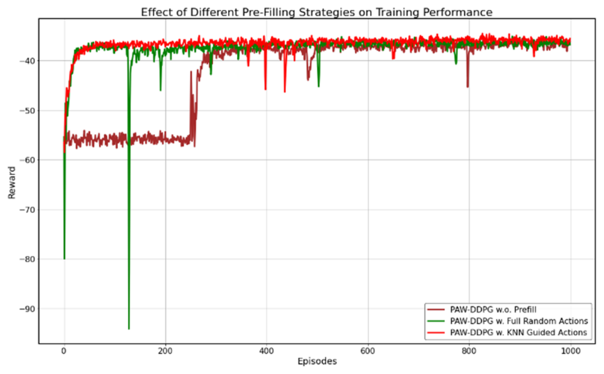
The objective of this phase is to accelerate the convergence process and improve the overall performance of the system. The technique adopted in this phase is initial pre-filling, where the main idea is to populate the ERB before starting the actual training process. In the conventional approach, DDPG algorithm begins to converge only after its ERB has been filled to its total capacity. This initial delay in convergence can lead to a slower overall optimization process, ultimately affecting the algorithm’s overall performance, particularly in situations where quick convergence is essential. To address this problem, this paper performs ERB initialization prior to training by pre-collecting experiences.

At the beginning, the agent selects actions randomly from the action space within the predefined bounds. The reason for using random actions initially is to ensure sufficient.

Exploration and to generate a diverse and unbiased set of experiences that cover different regions of the state–action space. After this prefilling step, the KNN algorithm is employed [46]. KNN is chosen because of its simplicity, effectiveness in capturing local similarities, and its ability to approximate values based on neighboring samples without requiring complex training. In this paper, KNN receives the current normalized state $s_i^{\prime }$ as input and produces the corresponding action $a_i$ by identifying the $\mathrm{Ҡ}$ most similar states stored in ERB. An inverse-distance weighting scheme is applied so that closer neighbors have a greater influence on the selected action, allowing more relevant experiences to contribute more significantly to the decision. The weighted average of KNN action at time slot $i$ is computed as:

$$a_i={\displaystyle \frac{{\sum }_{j=1}^{\mathrm{Ҡ}} \frac{1}{d_j+ \epsilon } a_j^{\left(i\right)}}{{\sum }_{j=1 }^{\mathrm{Ҡ}}\frac{1}{d_j + \epsilon }}}$$

(26)

where $a_i$ represents the action of the $j^{th }$ nearest neighbor at time slot $i$, $d_j$ denotes the distance to that neighbor, and $\mathrm{Ҡ}$ is the KNN neighbors. After the KNN algorithm predicts an action $a_i$ for each new normalized state $s_i^{\prime }$. The reward $r_i$ is then calculated using (21) with $w_1=w_2 =0.5$, and the next state $s_{i+1}^{\prime }$ is obtained. The corresponding transition $\left(s_i^{\prime },a_i,r_i,s_{i+1}^{\prime }\right)$ is stored in the ERB. At the same time, both the state and action datasets are updated iteratively.

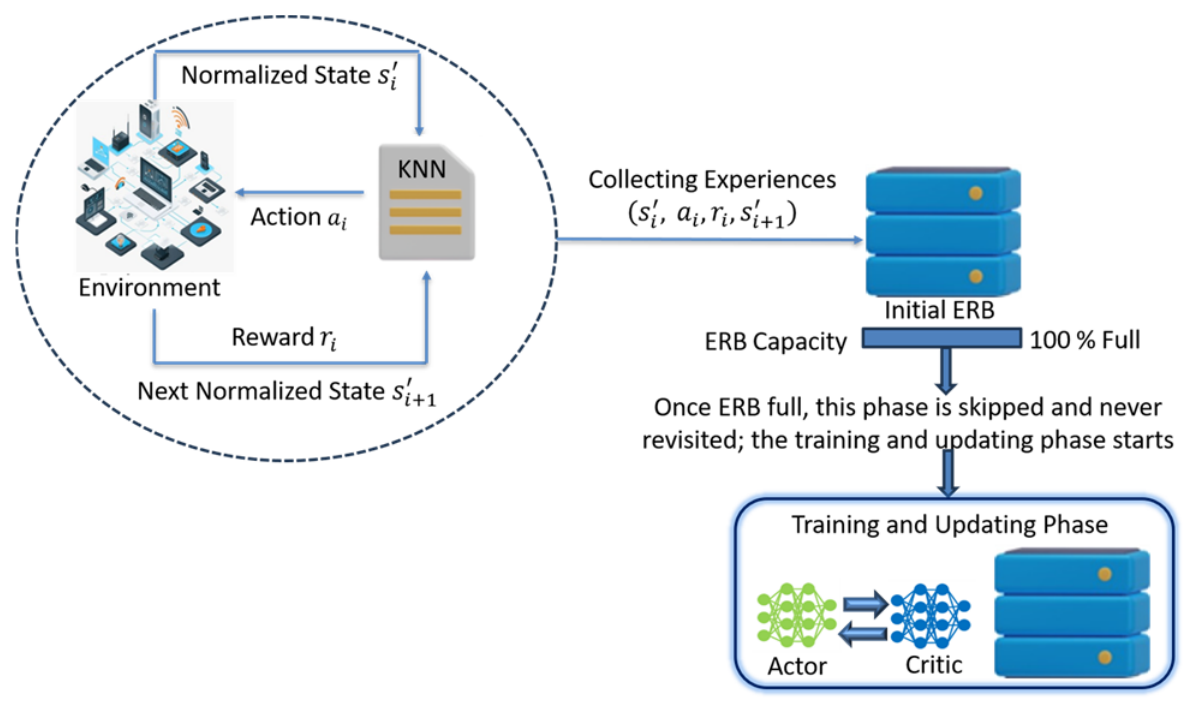
As shown in Figure 4, this pre-filling phase is executed only once, continuing until the ERB reaches its full capacity. Once the ERB is filled, the training process for the proposed PAW-DDPG algorithm begins, using the pre-filled, state-aware experiences to improve learning stability and convergence efficiency.

4.3.3. Phase 3: Training and Updating Phase

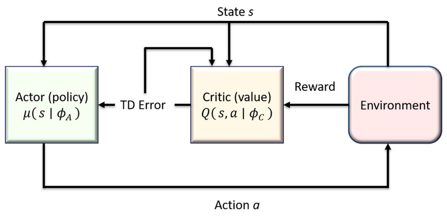
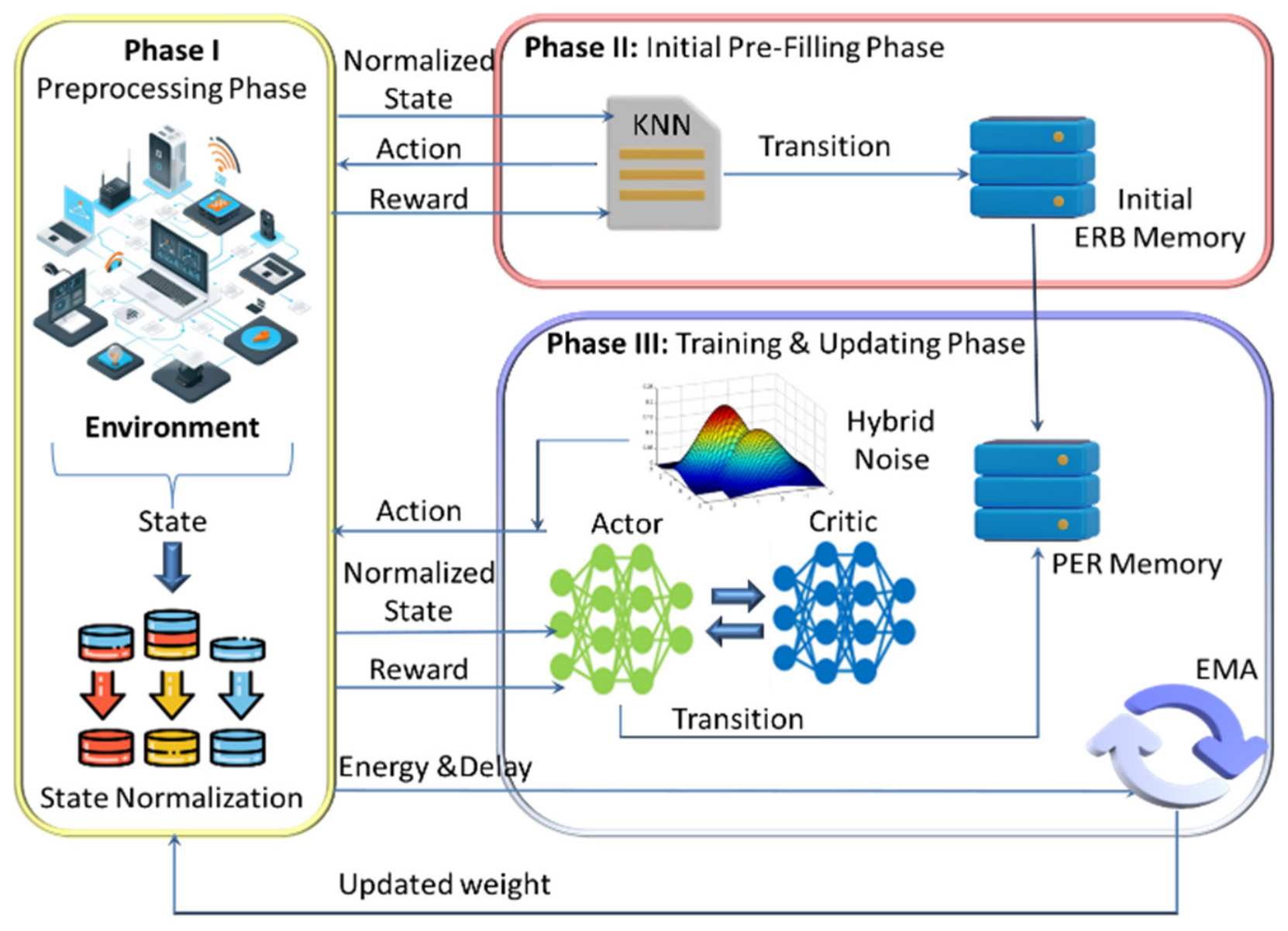
The main objective of this phase is to enhance the agent’s performance by improving exploration capability, learning efficiency, and overall training stability and convergence. The proposed PAW-DDPG algorithm relies on four networks: the actor network ${\varphi }_A$, which generates a deterministic action $a_i$ based on the current normalized state $s_i^{\prime }$; the critic network ${\varphi }_C$, which evaluates this action by estimating its Q-value; and their corresponding target networks $({\varphi }_A^{\prime }$, ${\varphi }_C^{\prime })$, which contribute to stabilizing the learning process. Although the actor produces deterministic actions, effective exploration remains essential to avoid convergence to suboptimal solutions. For this reason, noise is incorporated during training to encourage broader exploration of the action space and improve policy learning. After executing the action in the environment, both processing delay and energy consumption are obtained. These represent conflicting objectives and therefore require adaptive weighting consistent with the dynamic nature of the environment to determine the appropriate trade-off between them. The reward is then computed using (21). The next normalized state is also obtained. In each time slot $i$, the transition $\left(s_i^{\prime },a_i,r_i,s_{i+1}^{\prime }\right)$ is stored in ERB. Sampling mechanism from this ERB plays a critical role in stabilizing training [43].

All the exploration, reward function design, and sampling optimization methods significantly influence convergence behavior, learning stability, and overall system performance; therefore, enhancing these components is essential, and the following in this sub-subsection presents the improvements introduced to optimize their effectiveness.

1. 

Exploration optimization sub-phase

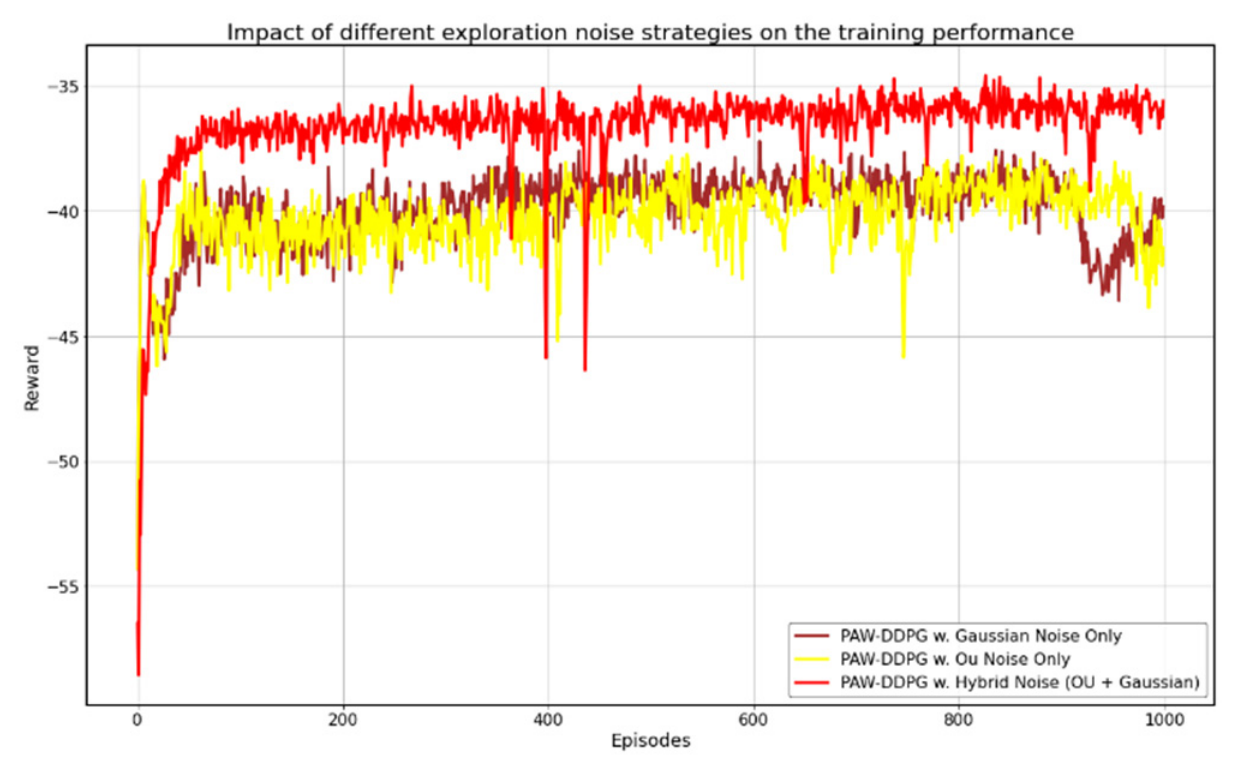
The objective of this sub-phase is to enhance the exploration capability of the proposed PAW-DDPG algorithm, which in turn improves convergence and consequently enhances the overall performance of the PAW-DDPG algorithm. In the conventional approaches, exploration is achieved by adding only Gaussian noise [42]. However, relying solely on Gaussian noise introduces purely random fluctuations that may lead to oscillatory behavior in the search trajectory. These random perturbations can cause instability, slow down convergence, and negatively affect the algorithm’s overall performance. To address this limitation, a hybrid noise strategy is proposed by combining Gaussian noise with Ornstein–Uhlenbeck (OU) noise. While Gaussian noise promotes broad and unbiased exploration due to its independent random distribution, OU noise introduces temporal correlation that generates smoother and more consistent exploratory movements [47]. The action space after adding hybrid noise is defined as:

$$a_i=\mu \left({s_i}^{\prime }∣{\varphi }_A\right)+\psi \cdot n_{OU}(i)+\beta \cdot n_G(i)$$

(27)

where $n_{OU}(i)$, $n_G(i)$ represents the OU noise and Gaussian noise, respectively, and $\psi$ and $\beta$ are weighting coefficients that control the contribution of each noise. The OU noise follows the stochastic differential equation:

$$n_{OU}\left(i+\Delta t_{OU}\right)=n_{OU}(i)+{\theta }_{OU}\left({\mu }_{OU}-n_{OU}(i)\right)\Delta t_{OU}+{\sigma }_{OU}\sqrt{\Delta t_{OU}}\hspace{0.17em}\mathcal{N}\left(\mathrm{0,1}\right)$$

(28)

where ${\theta }_{OU}$ is the rate of mean reversion, ${\mu }_{OU}$ is the mean value and ${\sigma }_{OU}$ controls the volatility of the process. The Gaussian noise component is sampled from a normal distribution as follows:

$$n_G(i)\sim N\left(0,{\sigma }_{\mathit{G}}^2\right)$$

(29)

where ${\sigma }_G$ is the standard deviation that determines the magnitude of the noise.

By integrating both types of noise, the algorithm benefits from both diverse global exploration (via Gaussian noise) and stable, correlated local exploration (via OU noise). Compared to using each noise type independently, the proposed combined noise approach reduces oscillations, improves convergence stability, accelerates convergence speed, and ultimately enhances the overall performance.

2. 

Adaptive weights update sub-phase

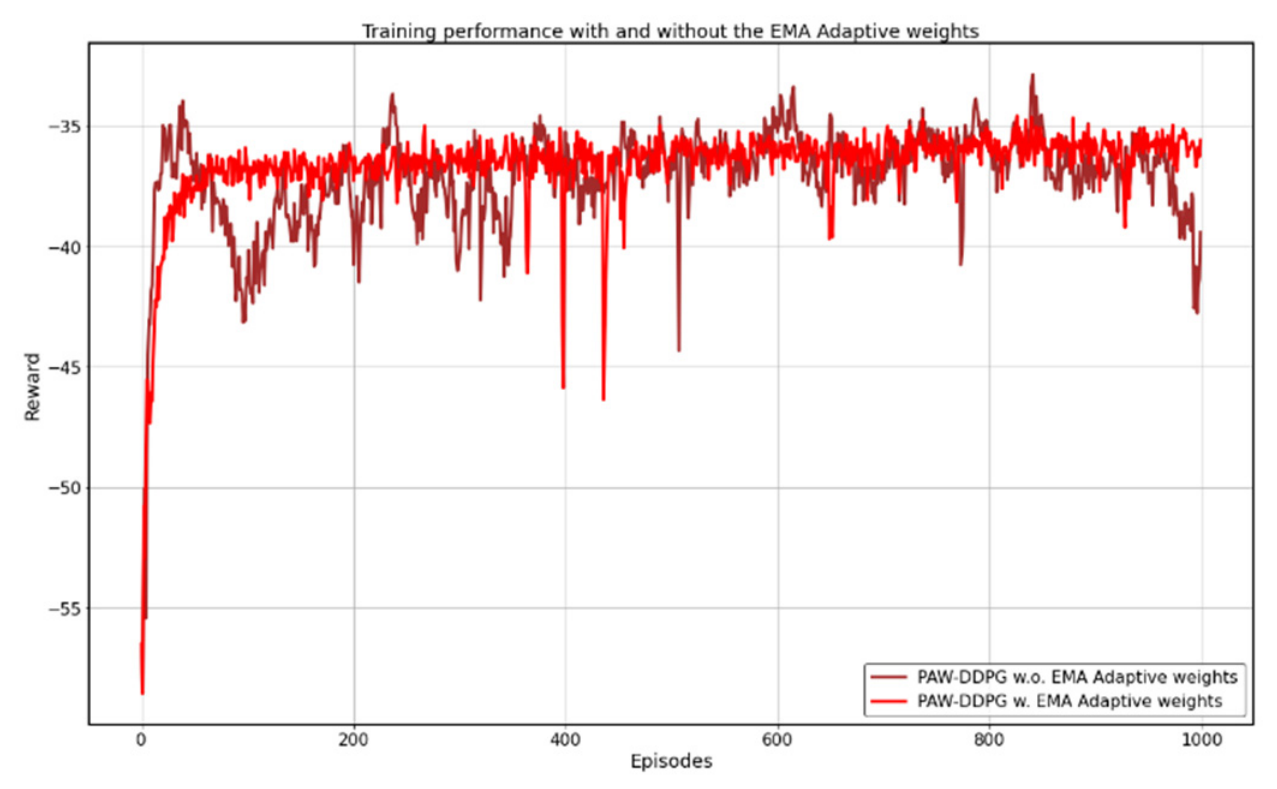
The purpose of this sub-phase is to improve stability and convergence by selecting optimal reward weights for delay and energy consumption. In RL–based optimization problems, especially in dynamic environments, the reward function often combines multiple conflicting objectives. In our paper, delay and energy consumption are weighted to balance performance and efficiency. Selecting appropriate weights is critical because they directly influence the agent’s learning direction, convergence speed, and overall system performance.

However, traditional methods typically rely on fixed or manually tuned weights. In dynamic environments, where network conditions, and resource availability vary over time, sudden or arbitrary weight selection can lead to unstable learning behavior. Abrupt changes in weights may cause oscillations in the reward signal, slow convergence, or even divergence. Moreover, poorly chosen weights may bias the agent excessively toward minimizing either delay or energy consumption, resulting in suboptimal performance. Such instability negatively affects policy convergence and reduces adaptability to environmental changes.

To address this problem, we adopt the EMA algorithm to adaptively determine the reward weights [48]. EMA provides a smooth and responsive mechanism for updating weights based on recent observations while still retaining historical information. Unlike abrupt or heuristic-based tuning methods, EMA ensures gradual transitions in weight values, which enhances learning stability and prevents sudden reward fluctuations. We select EMA over other adaptive methods because it is computationally efficient, easy to implement, and well-suited for real-time dynamic systems. Additionally, EMA inherently filters noise in the observed delay and energy metrics, contributing to more stable policy updates.

The weights for delay and energy consumption are selected at each episode and then applied across all time slots within that episode. This approach is a key design choice because it shifts the learning and optimization process to the episode level rather than operating independently at each time slot. The main advantage of this design is improved stability and convergence, especially in dynamic environments where per time-slot updates can introduce high variance and instability in learning.

Initially, all weights are assigned equal values to ensure a fair and unbiased starting point. These equal weights are then used during the first episode to evaluate baseline performance under consistent conditions. After completing the first episode, the EMA algorithm begins to refine the weights based on the observed outcomes, gradually improving performance over time.

After each episode, the current delay and energy are compared to their EMAs to calculate relative gaps, which quantify how much each metric deviates from its recent trend. These gaps are then compared, and the metric with the larger gap is considered worse, indicating that it requires more focus. Using this approach, the system adaptively prioritizes between delay and energy according to their relative performance, allocating resources to enhance the weaker metric. EMA and relative gap equations are represented as follows:

$$EM{A}_{delay}=\partial ·e{p}_{delay}+\left(1-\partial \right)·EM{A}_{delay}$$

(30)

$$EM{A}_{energy}=\partial ·e{p}_{energy}+\left(1-\partial \right)·EM{A}_{energy}$$

(31)

$$g_{delay}={\displaystyle \frac{e{p}_{delay}-EM{A}_{delay}}{EM{A}_{delay}+\epsilon }}$$

(32)

$$g_{energy}={\displaystyle \frac{e{p}_{energy}-EM{A}_{energy}}{EM{A}_{energy}+\epsilon }}$$

(33)

where $\partial$ is the EMA smoothing factor that controls how much weight is given to the current observation compared to the past average, ep denotes episode, and $\epsilon$ is a small constant to avoid division by zero.

Once the gaps are calculated, they are passed through a sigmoid function, which bounds extreme values between 0 and 1. This ensures that unusually large deviations do not dominate the weight calculation, creating a more stable adjustment process. The sigmoid function is applied as:

$$s_{delay}={\displaystyle \frac{1}{1+e^{-g_{delay}}}}$$

(34)

$$s_{energy}={\displaystyle \frac{1}{1+e^{-g_{energy}}}}$$

(35)

The resulting values are then used to compute target weights for processing delay and energy consumption as follows:

$$w_1^{target}={\displaystyle \frac{s_{delay}}{s_{delay}+s_{energy}}}$$

(36)

$$w_2^{target}={\displaystyle \frac{s_{energy}}{s_{delay}+s_{energy}}}$$

(37)

Before updating the weights, the EMA algorithm is enhanced by using soft update and momentum mechanisms to improve stability and learning efficiency during training. The main objective of these mechanisms is to gradually adjust the contribution of each weight according to the desired target behavior while avoiding sudden fluctuations that may negatively affect performance. Soft update mechanism is used as smoothing step. Instead of abruptly replacing the current weight with a new target value, the update blends the old value with the target using a smoothing factor $ᴦ$. This is computed as:

$$w_1^{new}=(1-ᴦ)w_1^{old} +ᴦ\hspace{0.17em}{w}_1^{target}$$

(38)

$$w_2^{new}=(1-ᴦ)w_2^{old}+ᴦ\hspace{0.17em}{w}_2^{target}$$

(39)

where $w_1^{old}$ = ${ w}_2^{old}$ = 0.5.

After that, momentum mechanism was introduced as an optimization mechanism that speeds up learning and stabilizes updates by combining the current gradient with a fraction of previous updates. Instead of relying only on the latest change, it accumulates past gradients, allowing the updates to maintain direction, move more smoothly, and converge faster with fewer oscillations:

$$w_1^{update}= m\cdot w_1^{update-prev}+\left(1-m\right)\hspace{0.17em}\left(w_1^{new}-w_1^{old}\right)$$

(40)

$$w_2^{update}=m\cdot w_2^{update-prev}+\left(1-m\right)\hspace{0.17em}\left(w_2^{new}-w_2^{old}\right)$$

(41)

where $m$ is the momentum coefficient. Together, these two mechanisms enhance convergence speed, improve robustness, and produce more reliable weight adjustments in dynamic environments.

3. 

Prioritized sampling sub-phase

The main objective of this sub-phase is to select a representative mini-batch of experiences from the ERB to improve learning efficiency, convergence speed, and overall system performance. An effective sampling method ensures that the most informative experiences contribute more significantly to the training process. The PAW-DDPG algorithm starts by using the normalized state as input to produce the corresponding action. Hybrid noise is then added to the action before executing it in the environment. Once the action is performed, the reward was computed by applying a weighted sum to the delay and energy consumption values, using weights obtained from the previous sub-phase. The next state, which is also normalized, is also obtained. This transition $\left(s_i^{\prime },a_i,r_i,s_{i+1}^{\prime }\right)$ is then stored in the ERB for future learning. These stored transitions form the ERB, from which samples are drawn to update the actor and critic networks.

The purpose of sampling from ERB is to break the temporal correlation between consecutive experiences and to reuse past interactions to improve data efficiency. In traditional ERB, transitions are sampled uniformly at random. While this approach stabilizes training compared to pure online updates, it treats all transitions as equally important. However, some experiences particularly those with large TD errors contain more learning information than others. Uniform random sampling may therefore slow convergence, as important transitions might be selected infrequently, reducing the speed at which the value function approximates the optimal solution.

To address this limitation, PER assigns higher sampling probability to transitions with larger TD errors [43,46]. The TD error represents the difference between the predicted Q-value and the updated target Q-value. It is mathematically defined as:

$${\delta }_{tr}=y_i - Q\left(s_i,a_i|{\varphi }_C\right)$$

(42)

where $y_i$ is the Q value of the target critic network, which was computed in (23) and $Q\left(s_i,a_i|{\varphi }_C\right)$ is the Q value of the output of the critic network. A large TD error indicates that the network’s prediction was inaccurate, meaning the transition carries significant learning information.

Instead of uniform sampling, each transition $tr$ at each time slot $i$ is assigned a priority $p_{tr}$, defined as:

$$p_{tr}={\left(\left|{\delta }_{tr}\right|+\epsilon \right)}^{\omega }$$

(43)

where ${\delta }_{tr}$ is the TD error of transition $tr$, $\epsilon$ is used to ensure that each experience has a nonzero probability of being selected, and $\omega \in [0, 1]$ controls how strongly priorities affect sampling, where $\omega =0$ ignores priorities completely and samples experiences uniformly at random and $\omega =1$ results in full prioritization based entirely on priority values [43].

The probability of sampling transition $tr$ at each time slot $i$ is then computed as:

$$P_{tr}={\displaystyle \frac{p_{tr}}{{\sum }_u{p}_u}}$$

(44)

where ${\sum }_u{p}_u$ refers to all stored transitions in ERB. By focusing on high-error transitions, PER accelerates error correction in the value function, which improves convergence speed and learning stability.

To correct the sampling bias introduced by prioritization, importance-sampling (IS) weights are utilized during gradient updates, which expressed as:

$$w_{tr}={\left({\displaystyle \frac{1}{Z\cdot P_{tr}}}\right)}^{\lambda }$$

(45)

where $Z$ is the replay buffer size, and $\lambda$ is a correction parameter that gradually increases to 1 to fully correct the bias.

After sample $N$ mini-batch, the critic network is updated at each time slot $i$ using a weighted mean squared error loss:

$$L={\displaystyle \frac{1}{N}}{\displaystyle \sum _{tr=1}^N}{w_{tr}\left({\delta }_{tr}\right)}^2$$

(46)

where $N$ is the batch size.

After the critic update, it guides the update of the actor network, encouraging the actor to select actions that maximize the expected reward according to the critic. The actor network is updated at each time slot $i$ through the deterministic policy gradient as follows:

$${\nabla }_{{\varphi }_A}J={\displaystyle \frac{1}{N}}{\displaystyle \sum _{tr=1}^N}\left[{\left.{\nabla }_{a}Q\left(s_i,a∣{\varphi }_C\right)\right|}_{a=\mu \left(s_i∣{\varphi }_A\right)}{ . \nabla }_{{\varphi }_A}\mu \left(s_i∣{\varphi }_A\right)\right]$$

(47)

To further stabilize training and improve convergence, the critic target network and actor target network softly updated by using a small constant $\tau$ as follows:

$${\varphi }_C^{\prime }\leftarrow \tau {\varphi }_C+\left(1-\tau \right){\varphi }_C^{\prime }$$

(48)

$${\varphi }_A^{\prime }\leftarrow \tau {\varphi }_A+\left(1-\tau \right){\varphi }_A^{\prime }$$

(49)

Algorithm 2 outlines the PAW-DDPG-based computation offloading and UAV trajectory control in UAV-assisted MEC system. The PAW-DDPG algorithm begins by initializing its networks: actor, critic, target actor, and target critic networks. After that, an initial pre_filling phase is performed, where the ERB is filled with more informative samples using the KNN algorithm in step 3. This step continues until the ERB is filled. Once the ERB is full, this step is terminated and is not revisited again. In the subsequent steps, the entire training process is carried out. The initial step is to determine the weights according to the EMA algorithm, starting with 0.5 and 0.5. The current state is normalized in step 9 and fed into the actor network, which outputs an action. Hybrid noise is then added to this action to generate the final action in step 10, which includes user scheduling, partial-task offloading and UAV trajectory and then executed in the environment, along with the next state in step 11. As a result, delay and energy are obtained, and from them the reward is calculated using the EMA weights values using (21) in step 12. The transition $\left(s_i^{\prime },a_i,r_i,s_{i+1}^{\prime }\right)$ are then stored in ERB with a priority in step 14. In steps 15–19, samples are selected from ERB using PER, and the networks are updated accordingly. At the end of each episode, the reward weights are dynamically computed in steps 21–26. These steps are repeated starting from step 5 until the training process is completed. 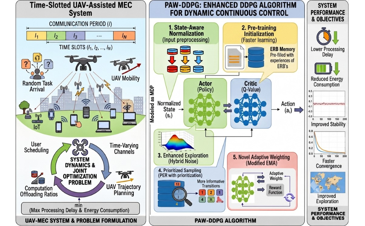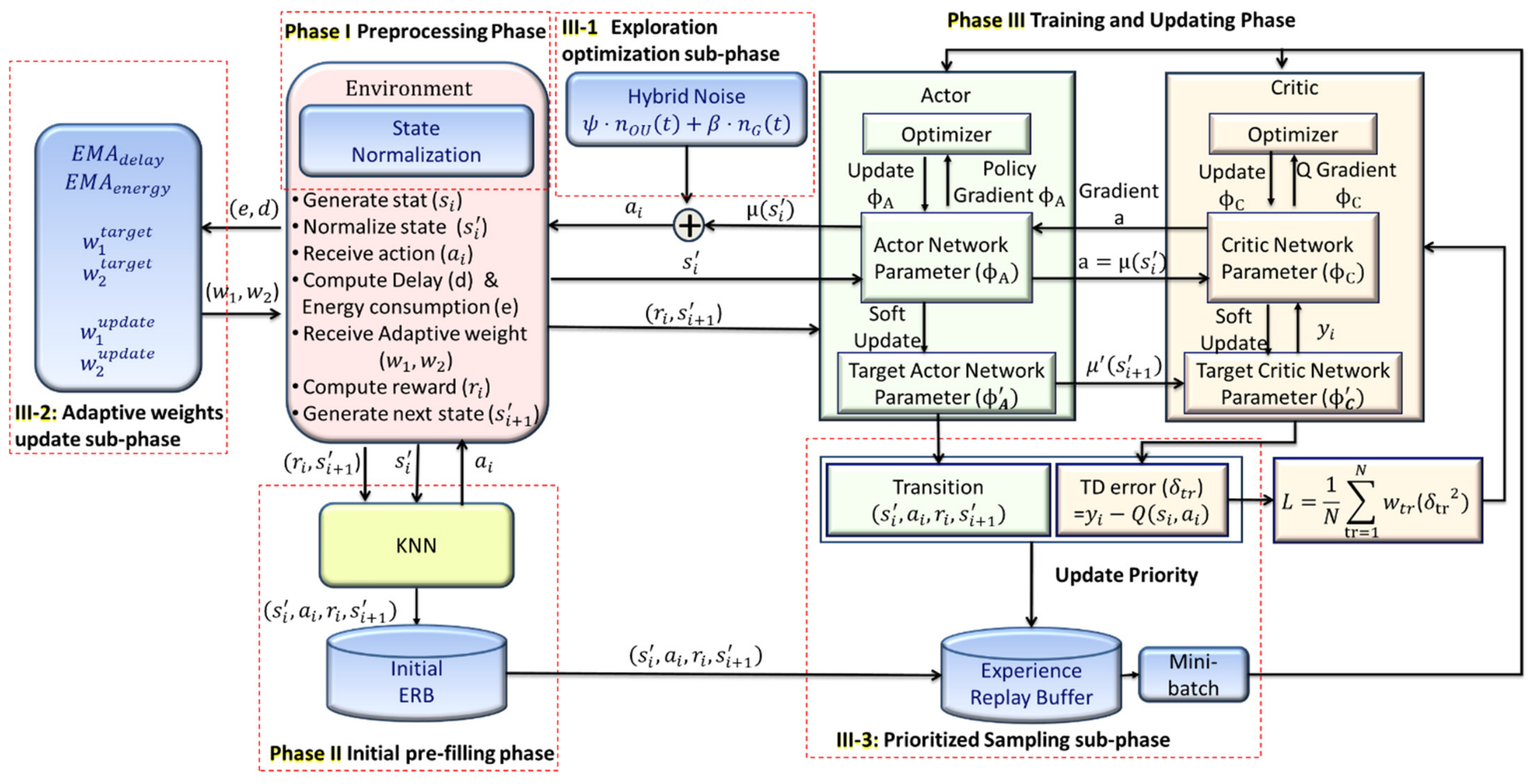Figure 5 depicts the proposed PAW-DDPG framework architecture, showing all the complete phases that were discussed.

Algorithm 2: PAW-DDPG-based computation offloading and UAV trajectory control

Input: Training episode length $E$, training sample length $I$, learning rates for actor and critic networks $({\alpha }_A, {\alpha }_C)$, discount factor $\gamma$, soft update rate $\tau$, ERB capacity, KNN parameters, hybrid noise weights $(\psi , \beta )$, mini-batch size $N$, EMA parameters.

Steps: 1.  Initialize the weights of actor network ${\varphi }_A$ and critic network ${\varphi }_C$, respectively 2.  Initialize the target networks with weights ${\varphi }_A^{\prime }\leftarrow {\varphi }_A$ and ${\varphi }_C^{\prime }\leftarrow {\varphi }_C$, respectively 3.  Initialize the ERB: Collect some random state–action pairs Build a KNN algorithm from these samples While the ERB is not full: ○ Obtain the current normalized state ○ If there are sufficient samples available, apply KNN to choose an action. If not, choose it random ○ Store transition $\left(s_i^{\prime },a_i,r_i,s_{i+1}^{\prime }\right)$ in the ERB ○ Add the new state–action pair to the KNN dataset Start training once the ERB is filled 4.  Initialize adaptive weights $w_1=w_2 =0.5$ 5.  for each episode $e \in \{\mathrm{1,2},\dots .,E\}$ do 6.       ${w_1=w}_1^{update}$ and ${w_2=w}_2^{update}$ 7.       Reset the environment and obtain the initial state $s_i$ 8.       for $i \in \{\mathrm{1,2},\dots .,I\}$ do 9.            Normalize the current state: $s_i^{\prime }$ = normalize state $(s_i$) 10.           Get an action $a_i$ with hybrid noise using Equation (27) 11.           Execute $a_i$ and move to next state $s_{i+1}$ 12.           Compute delay and energy consumption and obtain reward $r_i$ using Equation (21) 13.           Normalize the next state to obtain ${\mathrm{s}}_{\mathrm{i}+1}^{\prime }$ 14.           Store transition $\left(s_i^{\prime },a_i,r_i,s_{i+1}^{\prime }\right)$ in the ERB with priority $p_{tr}={\left(\left|{\delta }_{tr}\right|+\epsilon \right)}^{\omega }$ 15.           Sample a mini batch of $N$ transitions according to the PER probabilities using Equation (44) 16.           Compute target Q-values using Equation (23) 17.           Update the critic network by minimizing the loss using Equation (46) 18.           Update the actor network using the policy-gradient using Equation (47) 19.           Update the target networks using the soft update rule using Equations (48) and (49) 20.      end for 21.      Compute EMA of delay and energy using Equations (30) and (31) 22.      Compute relative performance gaps using Equations (32) and (33) 23.      Apply a sigmoid to convert gaps into stable, bounded importance scores using Equations (34) and (35) 24.      Build target weights from above importance scores using Equations (36) and (37) 25.      Apply a soft update to smooth weights using Equations (38) and (39) 26.      Enhance the weight update using momentum using Equations (40) and (41) 27. end for

5. Results and Analysis

This section presents the simulation results of the PAW-DDPG algorithm for joint user scheduling, partial-task offloading and UAV trajectory in UAV-assisted MEC systems. It begins by describing the parameters settings used in the simulation environment and network structure. Next, the effects of the proposed algorithm on system reward are evaluated. Then, the subsection discusses the influence of important hyper-parameters on the learning behavior and convergence performance. Subsequently, the proposed algorithm is analyzed in terms of training loss, computation rate, and average offloading ratio to verify its effectiveness and stability. Then, the proposed algorithm is compared with other baseline algorithms under different simulation scenarios to demonstrate its superiority in achieving balanced optimization between system delay and energy consumption. After that, the complexity of various algorithms is explained. Finally, the impact of the presence and absence of obstacles on the transmission rate is discussed.

5.1. Experimental Settings: Simulation Environment and Network Architecture

The proposed simulation considers 400 m × 400 m coverage area, where an UAV operates at a constant altitude of 100 m [38]. Initially, the UAV is located at the coordinates (200,100). There are $K$ = 4 UDs distributed randomly within a predefined coverage area [42]. The total computational task size is set to 100 Mbits [42]. The UAV’s mass is set to 9.65 kg, and its maximum speed is set to 20 m/s [38]. The UAV has a battery capacity of 500 kJ [46]. Wireless communication between the UAV and UDs is modeled over a 1 MHz bandwidth channel [35]. The total simulation period $T$ is 400 s, divided into equal and discrete time slots. Each time slot lasts for 10 s, resulting in a total of 40 time slots [38]. The computing capabilities are set to 0.6 GHz for UDs and 1.2 GHz for UAV [42]. The CPU energy consumption parameter is defined as ${10}^{-27 }$, and each bit of data requires 1000 CPU cycles for processing [42]. The noise power is defined separately for LoS and Non-Line-of-Sight (NLoS) conditions, with values of −100 dBm and −80 dBm, respectively. Uplink transmission power for each UD is fixed at 1 W [38], and the channel gain at reference distance is ${\alpha }_0$ = −50 dB at a reference distance of 1 m [42]. Each UD is randomly assigned a binary blockage indicator to model LoS/NLoS channel conditions. A weighted reward structure is employed, with equal emphasis on delay and energy consumption using $w_1$ = 0.5 and $w_2$ = 0.5. The comprehensive system parameters are listed in

Table 3. Simulation parameters.

Parameter	Value
$K$	4
$T$	400 s
$I$	40
$\mathbb{L}$	400 m
$W$	400 m
$H$	100 m
$m_{\mathit{uav}}$	9.65 kg
$v_{max}$	20 m/s
${\alpha }_0$	−50 dB
${\sigma }^2$	−100 dBm
$E_{\mathit{UAV}}$	500 KJ
$P_{\mathit{up}}$	1 W
$f_{\mathit{UD} k}$	0.6 GHz
$f_{\mathit{uav}}$	1.2 GHz
$s$	1000 Cycles/bit
$D$	100 Mbits
$t_{\mathit{fly}}$	2 s
$B$	1 MHz
ERB Capacity	10,000

.

The action space is constrained between −1 and 1 with an action dimension of 4. The state dimension is defined as 4 + 4 $K$, encompassing both UAV states and observations related to UD [2]. The architecture of the actor and critic networks used in this paper are presented in

Table 4. Architecture of actor and critic networks.

Network	Layer	Number of Neurons	Activation Function
Actor	Input Layer	20	N/A
	Hidden Layer1	400	Relu6
	Hidden Layer2	300	Relu6
	Hidden Layer3	10	Relu
	Output Layer	4	Tanh
Critic	Input Layer	24	N/A
	Hidden Layer1	400	Relu6
	Hidden Layer2	300	Relu6
	Hidden Layer3	10	Relu
	Output Layer	1	None

, where the actor is responsible for selecting actions based on the current state, while the critic network evaluates the action taken by the actor by estimating the expected Q(s, a) for a given state-action pair. Each network is composed of multiple layers, each containing a certain number of neurons, along with activation functions [49].

5.2. Reward-Based Performance Evaluation

This subsection presents the impact of state normalization on training stability and convergence speed is examined, followed by an analysis of the proposed PAW-DDPG algorithm integrated with KNN to demonstrate its effect on accelerating convergence and improving policy stability. This is followed by the evaluation of the hybrid noise strategy, which combines OU and Gaussian noises to enhance exploration efficiency. Finally, the impact of employing EMA for adaptive weights on performance convergence and overall system stability is evaluated.

Figure 6 illustrates the impact of applying state normalization on system reward and performance in the proposed PAW-DDPG algorithm. As shown, the agent trained with state normalization consistently delivers far higher and more stable rewards, clearly outperforming the agent trained without it. The average reward over 1000 episodes with normalization is −36.604, whereas without normalization it drops to −92.068. These results clearly show that state normalization substantially stabilizes the training dynamics, speeds up convergence, and protects the agent from diverging when feature scales are uneven. By scaling state features to a comparable numerical range, the agent can more effectively capture the underlying relationships between environment parameters, leading to faster learning and superior overall performance.

Figure 7 illustrates the effect of different pre-filling strategies on the training performance of the proposed PAW-DDPG algorithm. The results indicate that the absence of pre-filling leads to slower convergence, reflected in an average reward of −42.297 and a relatively high standard deviation 8.101, indicating higher variance in performance due to waiting for the ERB to be fully filled to its capacity before convergence begins. The inclusion of full random actions in the initialized ERB leads to a more stable learning process, enhanced convergence, and a higher average reward of −37.400 and reducing the variability 3.264. However, the best performance is achieved when the ERB is initialized using KNN guided actions, which leverage the similarity between current and past states to generate more informative and relevant experiences. This approach supplies a richer initial dataset, further boosting the average reward to −36.604 with the lowest standard deviation 1.822, reflecting both improved stability and faster convergence. Incorporating KNN guidance in the initial pre-filling phase significantly enhances the learning efficiency and policy robustness of the proposed PAW-DDPG algorithm compared to uninitialized or random ERB.

Figure 8 illustrates the impact of different exploration noise strategies on the training performance of the proposed PAW-DDPG algorithm. When relying solely on Gaussian noise, the average reward over 1000 episodes is −39.888, indicating a varied yet weakly correlated exploration pattern that causes abrupt action shifts and slows convergence. In contrast, OU noise only yields a slightly lower average reward of −40.254. Accordingly, both single-noise strategies demonstrate inherent limitations either generating excessive stochasticity or failing to deliver adequate exploratory diversity. The hybrid noise strategy (OU + Gaussian) overcomes these shortcomings by combining the complementary strengths of both noise types, where OU noise ensures smooth and temporally consistent exploration and Gaussian noise introduces additional stochastic variability. As a result, the hybrid noise achieves the highest average reward −36.604 with faster convergence and more stable learning dynamics, confirming its effectiveness in enhancing the overall training performance of the proposed PAW-DDPG algorithm.

Figure 9 shows the effect of adding the EMA algorithm as an adaptive weighting sub-phase. The algorithm without EMA adaptive weight adjustment based on performance feedback achieves an average reward of −37.131 with a standard deviation of 2.130, indicating moderate performance but noticeable fluctuations in stability. In contrast, the EMA-based adaptive algorithm achieves a higher average reward of −36.604 and a lower standard deviation of 1.822, demonstrating both improved learning efficiency and enhanced stability. This performance improvement confirms the role of the adaptive weighting sub-phase in dynamically balancing the trade-off between processing delay and energy consumption. By continuously adjusting the delay and energy weights based on real-time performance feedback, the algorithm maintains a balanced optimization focus. The EMA smoothing prevents abrupt weight changes, leading to more stable policy updates and faster convergence.

5.3. Impact of Hyperparameters Learning Behavior and Convergence

In this subsection, a set of hyperparameters are tuned, including the learning rate and the discount factor. Different values are tested for each hyperparameter to observe how they affect the algorithm’s performance. By experimenting with a range of configurations, we can better understand the sensitivity of the proposed PAW-DDPG algorithm to these parameters and identify the combination that leads to the most stable and efficient learning.

Figure 10 illustrates the performance of the proposed PAW-DDPG algorithm under different learning rate configurations for both the actor $\left({\alpha }_A\right)$ and critic $\left({\alpha }_C\right)$ networks. The learning rate is vital for influencing both the speed of convergence and the stability of training. As shown in the figure, no convergence is observed for the configurations (${\alpha }_A$ = 0.1, ${\alpha }_C$ = 0.2) and (${\alpha }_A$ = 0.01, ${\alpha }_C$ = 0.02), where the update steps are excessively large. In contrast, the configurations (${\alpha }_A$ = 0.001, ${\alpha }_C$ = 0.002), (${\alpha }_A$ = 0.0001, ${\alpha }_C$ = 0.0002), and (${\alpha }_A$ = 0.00001, ${\alpha }_C$ = 0.00002) achieve smoother convergence and more stable training. Among these, the best results are obtained at (${\alpha }_A$ = 0.001, ${\alpha }_C$ = 0.002), which provides the highest average reward of −36.604, followed by (${\alpha }_A$ = 0.0001, ${\alpha }_C$ = 0.0002), with −36.638, and (${\alpha }_A$ = 0.00001, ${\alpha }_C$ = 0.00002) with −38.458. Therefore, the learning rates ${\alpha }_A$ = 0.001 and ${\alpha }_C$ = 0.002 are identified as the optimal values for achieving efficient and stable convergence in the proposed PAW-DDPG algorithm.

Figure 11 illustrates the effect of different discount factors $\gamma$ on performance in terms of reward and convergence for the proposed PAW-DDPG algorithm over training episodes. In RL, the discount factor $\gamma$ regulates the trade-off between immediate and future rewards. As shown in the figure, higher discount factors such as $\gamma$ = 0.999 and $\gamma$ = 0.9 yield average rewards of −39.134 and −37.939, respectively, indicating slower convergence and greater fluctuation during early training due to the stronger focus on long-term optimization. Moderate values such as $\gamma$ = 0.7 and $\gamma$ = 0.6 improve performance, achieving average rewards of −37.058 and −36.880, respectively. However, the best result is obtained with a small discount factor of $\gamma$ = 0.001, which achieves the highest average reward −36.604 and the smoothest learning curve. Consequently, $\gamma$ = 0.001 is selected as the optimal discount factor, providing an effective balance between reward optimization and convergence.

5.4. Impact Training Convergence and System Efficiency Analysis

This subsection provides an analysis of the algorithm’s effect on essential performance metrics, such as training loss, computation rate, and average offloading ratio. By examining these indicators, we aim to demonstrate the effectiveness and efficiency of the proposed PAW-DDPG algorithm in optimizing system performance.

The training loss measures the accuracy with which the critic network predicts the Q-values for specific state-action pairs. It is defined as the mean squared error between the predicted Q-value and the target value generated by the target networks. A lower training loss indicates a more accurate approximation of the underlying value function, which contributes to more stable and effective updates of the actor policy [50]. Tracking this loss during training provides valuable insight into learning stability, and convergence progress. Figure 12 depicts the temporal evolution of training loss during the learning process. As shown, the training loss rapidly decreases at the beginning of training, indicating that the algorithm quickly learns to minimize prediction errors. After the initial sharp decline, the loss stabilizes near zero, suggesting that the critic network has effectively converged and the value estimation has become stable. The smooth convergence trend demonstrates steady learning progress and provides strong evidence of a stable and efficient training process.

The computation rate is an important measure used to evaluate the efficiency and performance of proposed PAW-DDPG algorithm. It refers to the number of computational tasks that the algorithm can perform per unit of time. A higher computation rate allows the algorithm to learn faster and handle more complex environments efficiently, while a lower rate may indicate slower training. The normalized computation rate is calculated by dividing the computation rate of the algorithm by the maximum computation rate observed, resulting in a value between 0 and 1 that represents utilization efficiency [50]. Figure 13 illustrates the normalized computation rate of the proposed PAW-DDPG algorithm of over 1000 episodes. As observed, the normalized computation rate increases rapidly during the initial phase of training, indicating a quick improvement in system performance as the algorithm learns more effective strategies. After approximately 200 episodes, the normalized computation rate stabilizes near its maximum value, indicating that the system has reached a steady-state operating condition. Minor fluctuations observed in later stages are due to dynamic environmental changes and adaptive policy adjustments.

The average offloading ratio is a key measure in evaluating the performance of partial offloading strategies in UAV-assisted MEC systems. It represents the average proportion of a computational task that is offloaded from a local device to a remote server for processing [42]. Monitoring this metric helps in understanding the balance between local computation and offloaded processing, optimizing performance, and improving efficiency. Figure 14 illustrates the variation in the offloading ratio of over 1000 training episodes. As observed, the offloading ratio is initially high, approximately 0.95, indicating frequent task offloading during the early stages of learning. As training progresses, the ratio gradually decreases and stabilizes around 0.60–0.65, reflecting the algorithm’s ability to adapt its offloading policy to achieve a better trade-off between computation delay and energy consumption. This trend suggests that the learning algorithm adapts its offloading decisions to balance system performance, leading to more stable and efficient behavior over time.

5.5. Comparative Performance Evaluation with Five Baseline Algorithms

This subsection aims to present a comprehensive comparison of the proposed PAW-DDPG algorithm with other five baseline algorithms to evaluate its performance and robustness. These baseline algorithms include:

• Local Only: All computational tasks are processed locally on the UDs without any offloading to UAV [2].
• Offload Only: All tasks are fully offloaded to the UAV for remote execution, with no local computation performed by UDs [2].
• DQN: DQN operates within a discrete action space and relies solely on value-based updates, limiting its performance in continuous environments [42].
• AC: AC employs a stochastic policy, which allows it to sample actions from a probability distribution. However, this stochastic nature can also slow down convergence, as the policy may take longer to consistently identify optimal actions [8].
• DDPG: The DDPG algorithm included the preprocessing phase; however, it waited for ERB to complete to start convergence. It mainly relied on Gaussian noise to generate an action, selected reward weights based on manually tuned weights, and sampled experiences at random [38,42].

To ensure a fair comparison, the algorithms including DQN, AC and DDPG apply state normalization. Figure 15 illustrates the reward performance of the six algorithms over 1000 training episodes under task sizes D = 100 Mbits. The proposed PAW-DDPG algorithm consistently achieves the highest reward, converging rapidly and maintaining a stable learning trend throughout the training process. Compared with the DDPG, the proposed algorithm results in a significantly faster convergence during the training process while also ensuring greater stability in the obtained rewards demonstrating the effectiveness of the introduced enhancements. These results indicate that the enhancements successfully enhance performance and lead to a more reliable and efficient learning process. The AC algorithm shows the most unstable learning behavior, with significant fluctuations and irregular convergence patterns, indicating its inability to maintain stable policy updates in dynamic environments. In contrast, DQN provides relatively stable but lower overall rewards, highlighting its limited capability to handle continuous control problems. The Offload Only algorithm yields lower overall rewards because it does not consider how resources are allocated, which may limit the overall system performance. Meanwhile, the Local Only algorithm consistently achieves the lowest performance since all computational tasks are executed locally, preventing the system from benefiting from the UAV’s offloading capability. The performance improvement of the proposed PAW-DDPG algorithm over the baseline algorithms is calculated using the following expression:

$$\mathrm{Improvement} \%={\displaystyle \frac{\mathrm{B}\mathrm{a}\mathrm{s}\mathrm{e}\mathrm{l}\mathrm{i}\mathrm{n}\mathrm{e} \mathrm{a}\mathrm{l}\mathrm{g}\mathrm{o}\mathrm{r}\mathrm{i}\mathrm{t}\mathrm{h}\mathrm{m}-\mathrm{P}\mathrm{r}\mathrm{o}\mathrm{p}\mathrm{o}\mathrm{s}\mathrm{e}\mathrm{d} \mathrm{a}\mathrm{l}\mathrm{g}\mathrm{o}\mathrm{r}\mathrm{i}\mathrm{t}\mathrm{h}\mathrm{m}}{\mathrm{B}\mathrm{a}\mathrm{s}\mathrm{e}\mathrm{l}\mathrm{i}\mathrm{n}\mathrm{e} \mathrm{a}\mathrm{l}\mathrm{g}\mathrm{o}\mathrm{r}\mathrm{i}\mathrm{t}\mathrm{h}\mathrm{m}}} \times 100$$

(50)

Based on this formulation, the proposed PAW-DDPG algorithm demonstrates substantial improvements compared with all baseline algorithms. Specifically, the proposed PAW-DDPG algorithm achieves performance gains in reward of 18.05%, 33.75%, 40.01%, 50.29%, and 61.73% over the DDPG, DQN, Offload Only, AC, and Local Only algorithms, respectively under task sizes D = 100 Mbits. These results clearly validate the effectiveness of the proposed enhancements in improving reward stability, convergence speed, and overall learning efficiency, confirming the superiority of the proposed PAW-DDPG algorithm for optimizing joint offloading and mobility decisions in UAV-assisted MEC systems.

The average reward, average delay, and average energy consumption of the six algorithms will be analyzed under different scenarios to evaluate their effectiveness and compare their outcomes. The performance of various algorithms under different task sizes ranging from 80 Mbits to 160 Mbits is compared in terms of average reward, average delay, and average energy consumption to evaluate how effectively they manage computational workloads. As shown in Figure 16a, the proposed PAW-DDPG algorithm consistently achieves the highest reward values under different task sizes. In contrast, the Local Only and AC algorithms yield the lowest rewards, indicating limited adaptability to increasing task demands. The DDPG, Offload Only, and DQN algorithms exhibit moderate performance but still fall short of proposed PAW-DDPG algorithm. From Figure 16b, we can see that the proposed PAW-DDPG algorithm consistently maintains the lowest delay under high load conditions, demonstrating its adaptability and faster convergence. As shown in Figure 16c, the proposed PAW-DDPG algorithm achieves better energy consumption under varying task sizes. It consistently outperformed the DDPG and Offload Only algorithms, with more significant improvements over the DQN, AC, and Local Only algorithms.

Table 5. Average reward values of PAW-DDPG and other algorithms across different task sizes.

Algorithm	Task Sizes (Mbits)
	80	100	120	140	160
Local Only	−84.010	−95.645	−95.645	−95.645	−95.645
Offload Only	−54.234	−61.020	−61.020	−61.020	−61.020
DQN	−48.914	−55.251	−48.825	−62.113	−54.688
AC	−57.793	−73.638	−73.713	−74.145	−58.480
DDPG	−51.220	−44.668	−42.648	−41.760	−41.976
PAW-DDPG	−42.132	−36.604	−36.646	−37.546	−40.131

,

Table 6. Average delay values of PAW-DDPG and other algorithms across different task sizes.

Algorithm	Task Sizes (Mbits)
	80	100	120	140	160
Local Only	139.810	157.311	157.311	157.311	157.311
Offload Only	89.187	100.732	100.732	100.732	100.732
DQN	77.761	86.698	74.596	97.589	85.650
AC	92.525	122.778	122.611	123.193	97.458
DDPG	84.315	66.478	65.139	64.608	64.442
PAW-DDPG	66.459	56.465	56.408	57.729	59.940

and

Table 7. Average energy consumption values of PAW-DDPG and other algorithms across different task sizes.

Algorithm	Task Sizes (Mbits)
	80	100	120	140	160
Local Only	30.199	33.979	33.979	33.979	33.979
Offload Only	19.282	22.071	22.071	22.071	22.071
DQN	22.085	24.820	23.452	26.114	24.641
AC	23.458	26.012	25.988	26.132	19.677
DDPG	18.921	22.609	20.407	19.991	19.964
PAW-DDPG	17.755	16.826	16.934	17.443	20.334

summarize the average values of reward, delay, and energy consumption for different task sizes, respectively, comparing the performance of the proposed PAW-DDPG algorithm with other algorithms. These findings confirm that the proposed enhancements significantly improve the learning efficiency and adaptability of the proposed PAW-DDPG algorithm under varying computational loads.

The performance of different algorithms as the UAV’s computing capability increases is also analyzed. By observing how the resulting average values of reward, delay, and energy consumption evolve with enhanced computational power, we aim to provide insights into which algorithms benefit the most from stronger onboard processing and which remain limited despite increased resources. As shown in Figure 17a, the proposed PAW-DDPG algorithm consistently achieves higher rewards compared to other baseline algorithms. Although most algorithms show a general enhancement in reward owing to faster task execution and lower computation delays, the proposed PAW-DDPG algorithm remains the most effective throughout the progressive increase in capabilities. From Figure 17b, we can observe that the proposed PAW-DDPG algorithm achieves the lowest delay compared with the baseline algorithms. Although increasing the UAV capability reduces the delay for most algorithms, the PAW-DDPG algorithm consistently provides the greatest improvement, outperforming the DDPG, Offload Only, DQN, and AC algorithms. As shown in Figure 17c, the proposed PAW-DDPG algorithm consistently achieves the lowest energy consumption compared to other baseline algorithms. It is clear from Figure 17 that the average values of reward, delay, and energy consumption of Local Only remain almost unaffected since all tasks are executed locally on UDs without utilizing UAV’s computing resources. These results demonstrate the superior effectiveness of the proposed PAW-DDPG algorithm in managing the trade-off between computation offloading and delay-energy performance. This behavior further confirms the advantage of adaptive offloading approaches like proposed PAW-DDPG algorithm, which can effectively leverage UAV computational power to achieve higher system efficiency in dynamic MEC environments.

Table 8. Average reward values of PAW-DDPG and other algorithms across different UAV computing capabilities (GHz).

Algorithm	UAV Computing Capability (GHz)
	0.8	1.0	1.2	1.4	1.6
Local Only	−95.645	−95.645	−95.645	−95.645	−95.645
Offload Only	−81.017	−68.869	−61.020	−55.203	−51.189
DQN	−62.669	−60.537	−55.251	−54.991	−55.017
AC	−87.297	−79.214	−73.638	−70.537	−49.422
DDPG	−51.983	−46.167	−44.668	−40.405	−38.212
PAW-DDPG	−47.317	−40.600	−36.604	−34.486	−34.236

,

Table 9. Average delay values of PAW-DDPG and other algorithms across different UAV computing capabilities (GHz).

Algorithm	UAV Computing Capability (GHz)
	0.8	1.0	1.2	1.4	1.6
Local Only	157.311	157.311	157.311	157.311	157.311
Offload Only	140.063	116.465	100.732	89.495	81.067
DQN	99.759	95.414	86.698	86.254	85.932
AC	146.278	132.682	122.778	116.109	78.794
DDPG	78.178	70.934	66.478	61.345	58.083
PAW-DDPG	72.308	62.693	56.465	52.352	50.373

and

Table 10. Average energy consumption values of PAW-DDPG and other algorithms across different UAV computing capabilities (GHz).

Algorithm	UAV Computing Capability (GHz)
	0.8	1.0	1.2	1.4	1.6
Local Only	33.979	33.979	33.979	33.979	33.979
Offload Only	22.071	22.071	22.071	22.071	22.071
DQN	27.266	26.535	24.820	24.820	24.820
AC	27.180	26.396	26.012	25.897	19.731
DDPG	24.828	21.726	22.609	19.596	18.337
PAW-DDPG	22.356	18.569	16.826	16.703	18.106

present the average values of reward, delay, and energy consumption for the PAW-DDPG algorithm and other algorithms under varying UAV computing capabilities.

The performance of various algorithms is evaluated under increasing UD computing capability. By observing the progression of average values of reward, delay, and energy consumption as users gain higher processing power, we seek to identify which algorithms can effectively leverage enhanced UD computation and which exhibit only limited improvement despite the enhanced resources. Figure 18a illustrates the variation in average rewards with respect to the computing capabilities of the UDs, ranging from 0.2 GHz to 0.7 GHz. The proposed PAW-DDPG algorithm consistently achieves the highest rewards across all capabilities, confirming its superior adaptability to varying computational conditions. The DDPG follows a similar upward trend but remains slightly below the proposed PAW-DDPG algorithm, indicating less optimization efficiency. The AC and DQN algorithms also show gradual improvement with increasing capability but still perform below the DDPG-based approaches because of slower convergence and limited control precision. The Local Only scheme exhibits significant improvement as the capability increases, since better local processing capability directly enhances task execution performance, yet it still yields much lower rewards compared to learning-based algorithms. According to Figure 18b,c, as the UD computing capabilities change, different algorithms show significant differences in terms of delay and energy consumption. The proposed PAW-DDPG algorithm demonstrates a relatively stable advantage in both delay and energy efficiency, with lower delay and energy consumption. The performance of the Local Only algorithm in terms of delay and energy consumption is highly sensitive to variations in UD computing capabilities. Increasing the UD computing capability reduces delay by improving local processing speed, but it also comes with an additional energy consumption cost. The AC and DQN algorithms show a reduction in delay as the UD computing capability increases, but their energy consumption exhibits a significant upward trend. In contrast, the Offload Only strategy remains constant across all capabilities, as its performance is independent of local computation capability. The figure demonstrates that higher UD computing capability enhances system performance for most adaptable algorithms, with the proposed PAW-DDPG algorithm maintaining the best results across different configurations.

Table 11. Average reward values of PAW-DDPG and other algorithms across different computing capabilities of UDs (GHz).

Algorithm	Computing Capabilities of UDs (GHz)
	0.2	0.3	0.4	0.5	0.6	0.7
Local Only	−237.855	−161.559	−125.534	−106.185	−95.645	−90.544
Offload Only	−61.020	−61.020	−61.020	−61.020	−61.020	−61.020
DQN	−147.449	−101.994	−77.534	−60.594	−55.251	−52.959
AC	−131.121	−59.963	−85.766	−77.907	−73.638	−72.900
DDPG	−66.586	−52.741	−46.792	−44.043	−44.668	−42.679
PAW-DDPG	−49.103	−48.411	−39.532	−36.587	−36.604	−38.212

,

Table 12. Average delay values of PAW-DDPG and other algorithms across different computing capabilities of UDs (GHz).

Algorithm	Computing Capabilities of UDs (GHz)
	0.2	0.3	0.4	0.5	0.6	0.7
Local Only	471.934	314.623	235.967	188.774	157.311	134.838
Offload Only	100.732	100.732	100.732	100.732	100.732	100.732
DQN	290.537	194.193	142.423	103.309	86.698	74.843
AC	249.345	100.760	153.404	135.567	122.778	113.517
DDPG	125.812	96.484	81.620	71.809	66.478	59.266
PAW-DDPG	87.868	86.967	67.907	60.172	56.465	53.761

and

Table 13. Average energy values of PAW-DDPG and other algorithms across different computing capabilities of UDs (GHz).

Algorithm	Computing Capabilities of UDs (GHz)
	0.2	0.3	0.4	0.5	0.6	0.7
Local Only	3.775	8.495	15.102	23.597	33.979	46.250
Offload Only	22.071	22.071	22.071	22.071	22.071	22.071
DQN	8.760	11.665	15.470	19.209	24.820	31.450
AC	12.920	19.432	17.531	21.247	26.012	31.946
DDPG	8.347	9.602	12.489	15.636	22.609	25.851
PAW-DDPG	10.184	9.687	11.140	13.061	16.826	22.708

summarize the average values of reward, delay, and energy consumption for different UD computing capabilities, respectively, comparing the performance of the proposed PAW-DDPG algorithm with other algorithms.

The performance of the different algorithms is compared as the number of UDs increases. By analyzing how average values of reward, delay, and energy consumption change as the system becomes more densely populated, we aim to uncover which algorithms scale effectively with an increase in users and which start to experience performance degradation under heavier network loads. Figure 19a illustrates the relationship between the number of UDs, and the average rewards obtained by various algorithms. The proposed PAW-DDPG algorithm consistently achieves the highest rewards across all UD configurations, confirming its superior learning capability and adaptability to dynamic network conditions. As shown in Figure 19b, the proposed PAW-DDPG algorithm demonstrates a relatively stable advantage in a lower delay. As shown in Figure 19a,b, the proposed PAW-DDPG algorithm, DDPG, Local Only, and Offload Only algorithms exhibit relatively stable and closely aligned performance, showing minimal variation as the number of UDs increases. This stability suggests that these algorithms are either inherently robust to changes in network size (as in the PAW-DDPG and DDPG) or follow fixed, non-adaptive behavior that remains unaffected by the number of devices (as in Local Only and Offload Only). In contrast, the AC and DQN algorithms display more pronounced fluctuations in average values of reward and delay, reflecting their sensitivity to varying system complexity and limited policy consistency. As shown in Figure 19c, the proposed PAW-DDPG algorithm achieves better energy consumption under varying number of UDs. The figure demonstrates that although increasing the number of UDs intensifies computational and communication challenges, the proposed PAW-DDPG algorithm maintains the most stable and superior performance across all algorithms.

Table 14. Average reward values of PAW-DDPG and other algorithms across different number of UDs.

Algorithm	Number of UDs
	1	2	3	4	5	6	7	8	9	10
Local Only	−95.670	−95.624	−95.590	−95.645	−95.632	−95.575	−95.620	−95.656	−95.583	−95.609
Offload Only	−61.847	−61.175	−61.601	−61.020	−61.474	−62.017	−62.109	−61.249	−61.076	−61.212
DQN	−78.796	−65.112	−54.826	−55.251	−49.454	−84.526	−76.388	−47.173	−64.992	−47.406
AC	−58.830	−58.672	−77.870	−73.638	−74.711	−75.239	−75.405	−74.356	−58.980	−59.302
DDPG	−43.005	−40.631	−43.078	−44.668	−40.545	−41.155	−41.339	−40.826	−41.008	−43.363
PAW-DDPG	−38.938	−40.936	−37.148	−36.604	−37.282	−37.796	−37.204	−37.807	−37.696	−37.842

,

Table 15. Average delay values of PAW-DDPG and other algorithms across different number of UDs.

Algorithm	Number of UDs
	1	2	3	4	5	6	7	8	9	10
Local Only	157.352	157.276	157.220	157.311	157.289	157.195	157.270	157.329	157.208	157.251
Offload Only	100.758	100.727	100.877	100.732	100.644	100.776	100.659	100.574	100.733	100.726
DQN	128.094	105.450	92.821	86.698	74.638	139.812	120.729	71.350	105.891	75.526
AC	97.225	97.004	128.254	122.778	123.738	124.011	124.849	123.445	97.687	97.868
DDPG	64.522	62.112	64.284	66.478	62.468	62.502	62.504	61.919	63.579	65.423
PAW-DDPG	58.242	60.600	56.710	56.465	57.234	57.809	57.030	57.619	57.757	58.222

and

Table 16. Average energy consumption values of PAW-DDPG and other algorithms across different number of UDs.

Algorithm	Number of UDs
	1	2	3	4	5	6	7	8	9	10
Local Only	33.988	33.972	33.960	33.979	33.975	33.954	33.970	33.983	33.957	33.966
Offload Only	22.140	22.032	22.226	22.071	21.946	22.136	22.042	21.936	22.089	22.067
DQN	29.185	26.281	17.755	24.820	24.142	30.168	30.174	22.346	24.554	18.187
AC	19.858	19.626	27.279	26.012	26.168	26.226	26.363	26.085	19.442	19.564
DDPG	21.682	19.471	21.471	22.609	19.286	19.800	18.843	19.093	18.960	21.532
PAW-DDPG	19.644	21.283	17.648	16.826	17.414	17.893	17.417	18.054	17.673	17.523

present the average values of reward, delay, and energy consumption of the PAW-DDPG algorithm and other algorithms under varying number of UDs.

5.6. Time Complexity Analysis of Comparative Algorithms

This subsection analyzes the time complexity of DQN, AC, DDPG, and PAW-DDPG algorithms. Assuming that $E$ is total number of episodes is, $I$ is total number of iterations per episode, $N$ is the batch size, $Z$ is the buffer size, and $\mathcal{P}$ is the number of neural network parameters.

• DQN: In each training iteration of DQN, two main operations are performed: (1) replay buffer sampling and (2) Q-network training. Replay buffer sampling is random, with complexity $O\left(N\right)$. Q-network training uses the sampled minibatch to perform forward and backward propagation for updating the network parameters, with complexity $O(N\times \mathcal{P})$. Consequently, the overall complexity of a single iteration is $O\left(N\right) + O(N\times \mathcal{P})$. Since $O\left(N\right)<< O(N\times \mathcal{P})$, the overall complexity is $O(E\times I\times N\times \mathcal{P})$.
• AC: In each training iteration of the AC algorithm, two main operations are performed: (1) actor network training and (2) critic network training. Training of both the actor and critic networks involves parameter updates, with complexities of $O\left({\mathcal{P}}_A\right)$ and $O\left({\mathcal{P}}_C\right)$, respectively. Therefore, the overall complexity of a single training iteration is $O({\mathcal{P}}_A + {\mathcal{P}}_C)$. Since actor and critic networks have similar architectures (${\mathcal{P}}_A\approx {\mathcal{P}}_C=\mathcal{P}$), the overall complexity is $O(E\times I\times \mathcal{P})$.
• DDPG: In each training iteration of DDPG, four main operations are performed: (1) replay buffer sampling, (2) critic network training, (3) actor network training, and (4) target network soft updates. Replay buffer sampling is random, with complexity $O\left(N\right)$. The computational complexity per update iteration is determined by the forward and backward propagation through the actor and critic networks. Critic network training uses the sampled minibatch for updating the critic network parameters, with complexity $O(N\times {\mathcal{P}}_C)$. Actor network training uses the sampled minibatch to perform for updating the actor network parameters, with complexity $(N\times P_A)$. Target network soft updates the parameters of the target actor and critic networks using a weighted average of the online network parameters, with complexity $O\left(\mathcal{P}\right)$. Since actor and critic networks have similar architectures (${\mathcal{P}}_A\approx {\mathcal{P}}_C=\mathcal{P}$), the overall complexity of a single training iteration is $O\left(N\right)+O(N\times \mathcal{P})+O\left(\mathcal{P}\right)$. Since the computational costs of updating the actor and critic networks dominate the replay buffer sampling and target network updates, the overall complexity is $O(E\times I\times N\times \mathcal{P})$.
• PAW-DDPG: Before the PAW-DDPG training process begins, a KNN-based pretraining initialization replay buffer is employed with informative experiences. Assuming $\mathrm{Ҡ}$ is the number of nearest neighbors, this phase has a complexity of $O(Z\times \mathrm{Ҡ}\times \mathcal{d})$, where $\mathcal{d}$ is the state-space dimension. This phase is used only until the replay buffer reaches its predefined capacity, after which it is no longer invoked. During each training iteration of the proposed PAW-DDPG algorithm, four main operations are performed: (1) PER sampling, (2) critic network training, (3) actor network training, and (4) target network soft updates. PER sampling selects a minibatch according to their priorities. Using a tree-based data structure, the sampling complexity is $O(N \mathrm{l}\mathrm{o}\mathrm{g} Z)$. The actor and critic networks updates remain identical to DDPG, with complexity $O(N\times \mathcal{P})$. The complexity of a single training iteration is $O(N \mathrm{l}\mathrm{o}\mathrm{g} Z)+ O(N\times \mathcal{P})$. The overall complexity is $O(Z\times \mathrm{Ҡ}\times \mathcal{d}) + O(E\times I\times (N \mathrm{l}\mathrm{o}\mathrm{g} Z+N \times \mathcal{P}\left)\right).$

Although PAW-DDPG adds extra overhead due to the pretraining initialization replay buffer and structured sampling, this increase is justified by the significant improvement in learning performance and convergence. Referring to Figure 15, it can be observed that the proposed PAW-DDPG algorithm converges remarkably fast from the very beginning of the training process, starting from the first episode. In contrast, the DQN and DDPG algorithms only begin to converge after 250 episodes. Moreover, the AC algorithm fails to converge over the entire training period because of the problem of simultaneous updating of the actor network and the critic network. The pretraining initialization replay buffer phase is used only until the replay buffer reaches its predefined capacity, after which it is no longer invoked. The prioritization mechanism allows the PAW-DDPG agent to learn from more important and diverse experiences instead of selecting samples randomly. As shown in Figure 15, avoiding random sampling improves the learning process, resulting in noticeably higher rewards compared with the other three algorithms.

5.7. Transmission Rate Analysis Under Dynamic Obstacles Scenarios

This subsection illustrates the transmission rate under LoS and NLoS communication conditions in the presence and absence of obstacles throughout the training process. Based on the description of channel transmission rate in Section 3.1, i.e., Equation (3), we can infer that obstruction directly affects the transmission rate between UDs and UAV. When an obstruction exists between the UD $k$ and the UAV, i.e., $b_{UD k}\left(i\right)=1$, the communication link operates under NLoS conditions. As shown in Figure 20, the transmission rate is significantly reduced due to the increased channel attenuation and signal blockage caused by the obstacle. Consequently, data transmission requires longer time, which may increase the overall delay. When there is no obstruction, i.e., $b_{UD k}\left(i\right)=0$, the communication link operates under LoS conditions. In this case, the transmission rate is considerably higher because the wireless channel experiences lower path loss and better signal quality. The higher transmission rate shortens the data transmission time, thereby reducing the communication delay and improving the overall efficiency of the UAV-assisted MEC system. Moreover, the fluctuations observed in both curves reflect the stochastic blockage model adopted in the proposed system, where the blockage status is randomly updated at each decision time slot to emulate sudden obstacle occurrences in a dynamic environment. Therefore, the proposed environment effectively captures the impact of dynamic obstacles on wireless communication, enabling the PAW-DDPG agent to continuously adapt its user scheduling, partial-task offloading decisions, and UAV trajectory according to the varying channel conditions.

6. Conclusions

This paper investigated the problem of user scheduling, partial-task offloading, and UAV trajectory in UAV-assisted MEC systems to serve multiple UDs with limited onboard resources. To address this problem, PAW-DDPG algorithm was proposed by incorporating a set of contributions that significantly enhanced stability, accelerated convergence, and improved overall performance to effectively handle dynamic environment. Specifically, state normalization mechanism is employed to enhance stability, while the KNN algorithm is utilized for effective ERB initialization, thereby speeding up the learning and convergence processes. The training and updating process is then used to enhance exploration through using hybrid noise scheme, improve stability and convergence by using EMA algorithm to achieve a balanced optimization between delay and energy consumption, and improve the efficiency of experience sampling through using PER algorithm. Simulation results showed that the proposed algorithm improved the performance by 60.24% with state normalization, 13.46% with ERB initialization, and 8.23% with hybrid noise. The results showed that the ERB initialization achieved 77.51% improvement in convergence and the EMA achieved 14.46%. Simulation results were conducted to analyze the effect of varying hyper-parameters, including the learning rate and discount factor. The effectiveness of the proposed algorithm was validated using performance metrics such as training loss, computation rate, and average offloading ratio, which demonstrate its superiority and stability. The results demonstrated that the proposed algorithm achieves notable improvements in terms of reward, delay, and energy consumption compared to baseline algorithms under task sizes D = 100 Mbits. Compared with DDPG, DQN, Offload Only, AC, and Local Only, the proposed algorithm achieves improvements in reward of 18.05%, 33.75%, 40.01%, 50.29%, and 61.73%, respectively, while decreasing delay by 15.06%, 34.87%, 43.94%, 54.01%, and 64.11% and reducing energy consumption by 25.58%, 32.21%, 23.76%, 35.31%, and 50.48%, respectively. A performance analysis in terms of average reward, average delay, and average energy consumption was also conducted for the proposed algorithm in comparison with baseline algorithms under different scenarios, where task sizes, UAV’s computing capability, UD computing capabilities, and number of UDs were varied. The results demonstrated that the proposed algorithm consistently outperformed the other algorithms across these different scenarios.

Future work may extend this framework to multi-UAV scenarios and incorporate more realistic mobility models. We will also focus on extending the proposed framework by incorporating explicit modeling and detecting sudden physical obstacles. The proposed enhancements can be integrated with more recent DRL algorithms, such as Soft Actor-Critic (SAC) and Twin Delayed Deep Deterministic Policy Gradient (TD3), to further improve exploration capability, convergence stability, and policy robustness. Comparative evaluations with state-of-the-art metaheuristic optimization methods and additional task offloading and resource allocation approaches will be conducted to provide a more comprehensive performance assessment under diverse dynamic MEC scenarios.