Classification Model of Emotional Tone in Hate Speech and Its Relationship with Inequality and Gender Stereotypes, Using NLP and Machine Learning Algorithms

Abstract

Hate speech on social media reproduces norms of inequality and gender stereotypes, disproportionately affecting women. This study proposes a hybrid approach that integrates emotional tone classification with explicit hostility detection to strengthen preventive moderation. We constructed a corpus from three open data sets (1,236,371 records; 1,003,991 after ETL) and represented the text using TF-IDF and contextual RoBERTa embeddings. We trained individual models (RoBERTa fine-tuned, Random Forest, and XGBoost) and a stacking metamodel (Gradient Boosting) that combines their probabilities. On the test set, the ensemble outperformed the base classifiers, achieving accuracy of 0.93 in hate detection and 0.90 in emotion classification, with an AUC of 0.98 for emotion classification. We implemented a RESTful API and a web client to validate the moderation flow before publication, along with an administration panel for auditing. Performance tests in a prototype deployment (Google Colab exposed through an Ngrok tunnel) provided proof-of-concept validation, revealing concurrency limitations from around 300 users due to infrastructure constraints. In general, the results indicate that incorporating emotional tone analysis improves the model’s ability to identify implicit hostility and offers a practical way to promote safer digital environments. The probabilistic outputs produced by the ensemble model were subsequently analyzed using the Bayesian Calibration and Optimal Design under Asymmetric Risk (BACON-AR) framework, which serves as a mathematical post hoc decision layer for evaluating classification behaviour under unequal error costs. Rather than modifying the trained architecture or improving its predictive performance, the framework identifies a cost-sensitive operating threshold that minimizes the total expected risk under the selected asymmetric cost configuration. The experiments were conducted using an English-language data set; therefore, the findings of this study are limited to hate speech detection in English.

1. Introduction

Hate speech is a complex phenomenon that undermines social harmony and equality in both physical and digital environments. Its definition involves at least three essential components: expressive behavior, a target group identified by protected characteristics, and the manifestation of negative emotions such as hostility, humiliation, or contempt [1]. However, establishing a universally accepted definition remains difficult, since the semantic and pragmatic particularities of the language introduce ambiguity in its interpretation [2]. Comparative studies also show that the conceptualization of hate speech varies in legal, cultural, and technological frameworks, reinforcing the need for multidimensional approaches to its analysis and detection [3].

The emotional dimension is key to understanding and detecting this phenomenon, as hate speech often draws on an affective background that shapes perception and social interaction. Basic emotions, such as happiness, anger, and fear, directly influence people’s social evaluations, even in the absence of contextual information [4]. Although emotions reflect immediate reactions, the emotional tone constitutes a more sustained affective state that modulates the interpretation of messages and their potential to become hate speech [5]. In the field of Natural Language Processing (NLP), the identification of emotions such as anger, contempt, or fear has been shown to improve the accuracy of automated systems in differentiating between negative opinions and discriminatory attacks [6,7].

Gender-based violence represents one of the most critical contexts in which hate speech manifests itself online. In Spanish-speaking communities, prior studies have identified that certain groups, including women, are more frequently targeted in specific forms of discriminatory discourse in which misogyny is reproduced through hostile expressions and patterns of social normalization [8]. On a global scale, online misogyny is associated with harassment dynamics that reinforce the structural subordination of women [9]; extreme forms of harassment, such as rapeglish, used for intimidation purposes have even been documented [10]. These dynamics motivate the development of more effective automated moderation systems capable of identifying both explicit and implicit hostility. However, the present study focuses on improving the technical performance of the detection models rather than conducting a subgroup-specific fairness analysis, which remains an important direction for future research [11].

In this context, Natural Language Processing (NLP) and Machine Learning (ML) are becoming established as fundamental approaches for detecting and mitigating hate speech. Systematic reviews highlight both their advances and limitations: dependence on large volumes of representative data, biases in training sets, and dilemmas regarding fairness and interpretability at scale [12,13]. The most promising results are observed in two families of models: (i) tree-based models (Random Forest, XGBoost) and (ii) transformative architectures, such as BERT and RoBERTa [14,15]. However, a significant gap remains: the explicit integration of emotional tone into the automated moderation process, especially before publication, which is the main motivation for this work.

From a formal perspective, we applied a mathematical model, Bayesian Calibration and Optimal Design Asymmetric Risk (BACON-AR) [16,17,18,19], which describes the relationship between textual features and hostility categories using a supervised probabilistic decision function. This model combines TF-IDF vector representations and RoBERTa contextual embeddings, integrated into an optimization process with L2 regularization and adaptive weights. The objective was to minimize classification errors and improve system stability, avoiding overfitting. Thus, the model formalizes the learning process from a statistical perspective, allowing us to analyze its convergence and generalizability in real-world hate speech detection scenarios. It is important to note that this study is based exclusively on an English-language data set; therefore, the proposed approach is limited to English hate speech detection and may not generalize to other languages without further adaptation.

From this perspective, the present study strengthens preventive moderation on social networks through a hybrid approach that combines the detection of explicit hostility with the classification of emotional tone. The main contributions of this study are as follows.

• The development of a dual model that simultaneously classifies hate/non-hate categories and emotional tone, implemented via a stacking assembly that integrates RoBERTa, Random Forest (TF-IDF), and XGBoost (embeddings), surpasses the performance of individual classifiers;
• The construction and enrichment of an extensive corpus from three open sources, with a mapping between GoEmotions and Ekman’s emotions to study the interaction between affect and hostility;
• An end-to-end functional validation using a RESTful API and a web client with pre-moderation and auditing.

This study presents a comparative analysis that explores the contribution of emotional tone to hate speech detection, evaluating whether the integration of affective signals with semantic representations improves the robustness of the classification process in ambiguous or context-dependent cases.

These contributions complement studies that warn about bias risks and implementation challenges [13,20] and confirm that a heterogeneous ensemble (transformer plus trees) improves generalization compared to the isolated use of a model such as RoBERTa [14].

The remainder of the manuscript is structured as follows: Section 3 describes the corpus, preprocessing, feature representation, models, the API, and web client architecture. In this section, we also incorporate the BACON-AR framework for probabilistic calibration and threshold optimization under asymmetric risk. Section 4 presents model performance, ROC curves, confusion matrices, and performance tests. Section 5 analyzes the findings, validates and discusses limitations. Finally, Section 6 summarizes the contributions and future research directions.

2. Related Work

We conducted a Systematic Review of the Literature (SLR) following the PRISMA guidelines and the PICOS approach, thus identifying the most relevant studies on the detection of hate speech and the analysis of emotional tone, published in [21]. We searched various recognized scientific databases, filtering by language, year of publication, and research approach. We analyzed 34 primary studies and selected 10 representative works. In addition, we include five recent studies that broaden the analysis to include multimodal approaches and the use of large-scale language models (LLMs).

To facilitate a clearer comparison between existing approaches and the proposed hybrid model,

Table 1. Comparison of representative hate speech detection approaches in the literature.

Study	Method	Reported Performance	Limitations
Min et al. (2023) [22]	Self-training multi-label model with emotional cues	Improved sensitivity to implicit hostility	Limited interpretability and dependence on labeled data
Rodríguez et al. [23]	FADOHS framework integrating sentiment and emotion	Improved performance over lexical models	Focused mainly on sentiment features
Kaminska et al. (2023) [24]	Fuzzy-rough k-NN classifier	Competitive performance with small data sets	Limited scalability for large corpora
Keya et al. (2023) [25]	G-BERT transformer model	High accuracy in low-resource language	Language-specific training limits generalization
Paul et al. [26]	Multimodal cross- attention model	Improved contextual understanding	Requires multimodal data availability
Guo et al. (2021) [27]	Evaluation of Large Language Models	High accuracy in supervised settings	Bias replication and over-detection of hostility
Proposed approach	Hybrid stacking ensemble (RoBERTa + Random Forest + XGBoost) with emotional tone classification	Improved robustness in detecting hostility and emotional tone	Prototype validation; large-scale deployment requires dedicated infrastructure

summarizes representative studies, highlighting their methods, data sets, reported performance, and main limitations.

In [22], the authors proposed a multi-label self-training model that combines auxiliary emotional cues to improve the sensitivity of automated systems to implicit hostility on social networks. This work demonstrated that negative emotions, such as anger and contempt, strengthen the identification of discriminatory discourse. Ramos et al. [28] analyzed the evolution of transformer-based models and highlighted the limitations in the explainability and bias of current detection systems, underscoring the need to develop more interpretive approaches. Rodriguez et al. [23] presented the FADOHS framework, which integrates sentiment and emotion analysis to classify offensive Facebook posts, finding that combining affective and linguistic cues improves performance over purely lexical methods. Finally, Kaminska et al. [24] proposed a fuzzy-rough k-NN method for the simultaneous identification of hate, irony, and emotion, demonstrating the usefulness of non-transformer-based techniques in contexts with limited data.

In the Spanish context, ref. [29] developed a model that incorporates user linguistics and features to detect offensive messages, highlighting the relevance of sociocultural context in the classification of hate speech. Complementarily, ref. [30] introduced the Spanish MTLHateCorpus 2023, which uses a multitask approach to predict the type, target group, and intensity; this resource facilitates the study of social and gender inequality in digital environments. Ref. [26] proposed a multimodal cross-attention model that combines text and image for hostility detection, demonstrating that the integration of visual and semantic information allows capturing nuances that text alone does not reflect. Ref. [25] presented G-BERT, a Bengali-trained hate speech detection model that addresses the challenges of languages with limited computational resources. Ref. [31] analyzed the emotional classification in code-mixed texts (Hinglish). Meanwhile, ref. [32] designed a multitask model that links politeness and emotion in social interactions, thus facilitating the transfer of affective tasks.

Among recent studies, Nandi et al. [33] introduced SAFE-MEME, a structured reasoning model for detecting hate speech in memes that incorporates emotional attention and semantic relationships between text and images, thus improving contextual interpretation. Chhabra and Vishwakarma [34] proposed MHS-STMA, a multilevel attention transformer-based framework that simultaneously processes textual and visual modalities, achieving greater precision and robustness in the face of data noise. Complementarily, Chhabra and Vishwakarma [35] demonstrated that multiscale visual attention improves the detection of hostility in images with superimposed text, reaffirming the importance of integrating visual features to address implicit hate speech in multimodal content.

Furthermore, ref. [27] evaluated various large language models (LLMs) to detect hate speech in real-world settings, analyzing their generalizability and the influence of cultural context on decision-making. The authors found that while LLMs achieve high accuracy in supervised tasks, they tend to replicate social biases and over-identify neutral expressions as hostile. Ref. [36] extended this analysis to multilingual contexts with high semantic variability, where the models demonstrated inconsistencies in transferring hostility patterns between languages, reinforcing the need for control and calibration mechanisms. Finally, ref. [37] examined the reactive responses of LLMs to offensive content, finding that these models reproduce stereotypes and degrade their performance with ambiguous or ironic texts, highlighting limitations in their reliability and algorithmic fairness.

Complementing this evolution towards hybrid and multimodal architectures, two recent systematic reviews consolidate the theoretical foundation of the present research. On the one hand, ref. [38] conducted a literature review on hate speech detection on online social networks using Machine Learning and Natural Language Processing, identifying the main techniques, data sets, and challenges in this field. On the other hand, we conducted a systematic review of emotional tone detection in hate speech, published in [21]. This latter study not only maps the current methods and challenges but also underscores the research opportunity addressed by the present work: the explicit integration of the emotional component to improve the accuracy and contextual understanding of automated moderation systems.

In summary, the analyzed works demonstrate an evolution towards hybrid and multimodal architectures, although most focus on English-language general hostility detection. Given these limitations, the present study proposes a complementary approach. It uses an English corpus with over one million records, labeled according to Ekman’s six basic emotions. The model combines hate speech detection and emotional tone classification using a stacking scheme composed of three configurations: RoBERTa as the base model, XGBoost with TF-IDF features, and a Random Forest with RoBERTa-generated embeddings. This approach contrasts contextual and statistical representations to improve the accuracy and interpretability of the results. Furthermore, the implementation in a RESTful API and a web client demonstrates its applicability in automated moderation processes and large-scale content analysis.

Taken together, the reviewed studies support the incorporation of the emotional component into hate detection. The proposed approach contributes to this line of research by integrating natural language processing, emotions, and gender inequality, with the aim of developing more accurate and socially relevant automated moderation systems.

Several recent studies have provided fundamental theoretical and mathematical foundations for detecting hate speech using probabilistic models. In particular, refs. [39,40] analyze classifier calibration and probabilistic prediction evaluation, highlighting the importance of adjusting model reliability via loss functions and decision thresholds. Complementarily, refs. [16,17] propose Bayesian frameworks that allow the representation of uncertainty in predictions and improve the stability of deep learning systems under variable conditions.

Furthermore, refs. [41,42] delve deeper into cost-sensitive learning, introducing formulations that optimize the hazard function in scenarios with unbalanced classes or decisions that involve different penalty levels. These perspectives, along with the regularization and error control strategies proposed by refs. [18,19], provide the mathematical foundation for the approach used in this study.

The proposed model builds on these contributions by integrating a statistical calibration process into a hybrid classification framework based on trees and transformers. This formulation combines vector representations of text (TF-IDF and contextual embeddings) with calibrated probabilistic estimates, seeking to optimize the accuracy, consistency, and reliability of the hostility and emotional tone detection system.

3. Materials and Methods

3.1. Data Set

We constructed a data set comprising 1,236,371 records integrating three open-access data sets obtained from Kaggle to detect hate speech on social media. Each data set contained the comment and binary detection of hate/non-hate, as detailed in

Table 2. Data sets used for the training and evaluation of the models.

Data Set	Number of Records
Hate Speech Detection curated data set	417,561
Detection of implicit beliefs of gender violence against women on social networks using NLP algorithms and machine learning classification techniques	510,254
HateXplain	308,556

.

Next, we combined the three data sets to obtain the final data set. In this corpus, we applied a pre-trained model RoBERTa-base-go_emotions, to map Ekman’s six basic emotions (i.e., anger, fear, sadness, surprise, disgust, and joy) plus the emotion of neutral to each comment, as shown in

Table 3. Mapping of GoEmotions emotions to Ekman’s basic emotions.

Ekman Emotion	Associated GoEmotions Emotions
Neutral	admiration, amusement, approval, love, gratitude, pride, neutral
Joy	caring, desire, excitement, optimism, relief
Anger	annoyance, anger
Disgust	disapproval, disgust, remorse
Fear	fear, nervousness
Sadness	disappointment, embarrassment, grief, sadness
Surprise	confusion, realization, curiosity, surprise

; this resulted in a data set with three labels: comment, hate speech detection, and emotion classification.

Manual Validation of Emotion Labels

It should be noted that emotion labels are pseudo-labels, not human reference annotations, as they were generated using the pre-trained RoBERTa GoEmotions model. Therefore, to assess the reliability of these labels, we manually validated a random sample of 200 comments from the data set.

Each comment was independently evaluated by two annotators with backgrounds in software engineering and experience in natural language processing. Both annotators analyzed whether the emotion predicted by the model matched the emotional tone perceived in the text. In cases of disagreement, a consensus was reached through discussion to ensure the consistency of the final annotation.

This validation process allowed us to calculate the agreement rate between the model-generated labels and the human assessment. To quantify this level, we used the metric defined in Equation (1).

$$Agreement={\displaystyle \frac{N_{match}}{N_{total}}}\times 100$$

(1)

where $N_{match}$ represents the number of matches between the emotion predicted by the model and the emotion manually reviewed, and $N_{total}$ corresponds to the total number of comments evaluated.

We obtained 170 matches out of 200 reviewed comments, corresponding to an agreement rate of 85.00%, as shown in Equation (2).

$$Agreement={\displaystyle \frac{170}{200}}\times 100=85.00\%$$

(2)

In addition, the number of discrepancies between the model-generated labels and the manual review was calculated using Equation (3).

$$N_{mismatch}=N_{total}-N_{match}$$

(3)

In this case, we identified 30 discrepancies between the labels generated by the model and the manual review, indicating the presence of errors in the pseudo-labels. To complement this evaluation, we calculated Cohen’s Kappa coefficient to measure the level of agreement considering the effect of chance. This coefficient is defined in Equation (4).

$$\kappa ={\displaystyle \frac{P_o-P_e}{1-P_e}}$$

(4)

We calculated the observed agreement as $P_o=170/200=0.85$. Then, we obtained the expected agreement by chance ($P_e$) from the marginal distributions of the classes in the manual and model labels. To do this, we multiplied the corresponding frequencies of each emotion and divided the result by the total number of squared samples. As a result, we obtained $P_e=0.6053$.

Finally, we substituted these values into the equation and obtained $\kappa =0.62$, which indicates a substantial level of agreement between the model predictions and the manual validation.

These results are supported by the actual distribution of the classes, where the dominant emotion Anger accounts for the majority of observations, which directly influences the value of the expected agreement by chance ($P_e$).

Table 4. Marginal distribution of emotions in manual and model labels.

Emotion	Manual	Model
Anger	148	159
Disgust	27	20
Surprise	10	6
Happiness	8	8
Sadness	3	2
Fear	3	3
Neutral	1	2
Total	200	200

presents the frequencies used for this calculation.

The manual validation results provide quantitative evidence of the consistency between the pseudo-labels generated by the model and the human assessment. In particular, the evaluation includes both the raw agreement percentage and the Cohen’s Kappa coefficient, which accounts for agreement beyond chance.

Table 5. Summary of the manual validation of emotional pseudo-labels.

Metric	Value
Total comments evaluated	200
Model–manual review matches	170
Non-matches	30
Agreement percentage	85.00%
Cohen’s Kappa	0.62

presents a summary of the results obtained in the manual validation process.

The results show agreement between the emotion labels generated by the model and the manual review, with an agreement rate of 85%. This value indicates that the majority of pseudo-labels are consistent with human interpretation, although a non-negligible proportion of discrepancies (15%) remains.

Furthermore, the Cohen’s Kappa value of 0.62 indicates a substantial level of agreement beyond chance, according to standard interpretation ranges. This result confirms that the observed agreement is not solely due to class distribution effects but reflects a meaningful correspondence between the model predictions and human judgment.

Furthermore, based on the class analysis, we identified that most errors are concentrated in less-represented emotions such as Surprise, Sadness, and Fear, while the dominant emotion, Anger, shows a high level of agreement. This demonstrates the effect of class imbalance on model performance.

Although a high level of agreement is observed, there is a significant limitation. Since the labels were generated by a pre-trained model and subsequently used to train the emotion classifier, there is a risk of bias propagation. Therefore, the results should be interpreted with caution, and future work should incorporate fully human-annotated data sets and more robust validation metrics.

3.2. Preprocessing—ETL

For the extraction, transformation, and loading (ETL) process, we applied several normalization steps, including the removal of duplicates and null values, character normalization to convert comments to lowercase, and the removal of non-textual elements such as emojis, hashtags, and symbols. Although emojis can convey relevant emotional signals in social media communication, they were removed to ensure a consistent textual representation in the heterogeneous data sets integrated in this study, since some of the source corpora do not systematically preserve emoji information.

The proposed models rely primarily on semantic textual representations derived from TF-IDF features and contextual embeddings generated by RoBERTa, which capture emotional and contextual patterns directly from the textual content. Therefore, the emotional tone classification task is mainly driven by linguistic and contextual cues present in the text rather than by graphical elements such as emojis.

To ensure data integrity, we checked for duplicate records after combining the three data sets. This procedure allowed us to identify and remove repeated comments that might appear in multiple data sets. In this way, we reduce the risk of overestimating the model’s performance.

After completion of the process, we obtained 1,003,991 clean records, which we used for training and validation.

3.3. Exploratory Data Analysis—EDA

Using the clean data set, we conducted an exploratory data analysis to identify trends, patterns, label distributions, and potential biases. In this case, we evaluated the proportion of records classified as hate/non-hate, finding a balance: 502,159 records in the non-hate class and 501,832 in the hate class, as shown in Figure 1.

We also found a bias in the distribution of emotions in the data set, as shown in Figure 2. We observed a predominance of emotions such as anger (564,191), disgust (207,469), and joy (137,686), while the least represented were surprise (14,637), fear (21,577), and neutral (24,345), resulting in an imbalance between the different classes, which poses a challenge in the model training process.

To mitigate class imbalance during training, we applied a class weighting scheme. This assigns a greater penalty to errors associated with minority classes and reduces bias toward dominant classes such as anger or disgust. In this way, the models learn patterns representative of the less frequent emotions present in the data set. Furthermore, during model evaluation, we used macro-averaged metrics (i.e., precision, recall, and F1 score) to ensure equal weighting across all classes.

3.4. Feature Representation

For the representation of textual features, we applied two approaches:

• Contextual Embeddings: generated using the pretrained model cardiffnlp/twitter-RoBERTa-base, which transforms each comment into a 768-dimensional vector that captures semantic and contextual information from the text.
• TF-IDF (Term Frequency–Inverse Document Frequency): a technique to assess the importance of each word within the corpus, to obtain a representation based on normalized term frequencies [43].
  For TF-IDF vectors, we calculate them using the normalization l2, corresponding to the default configuration of the TfidfVectorizer implementation.

3.5. Selection of NLP and ML Models

We implemented and compared traditional and modern NLP models. Within the NLP model, we selected the RoBERTa model because it is commonly used for text classification, natural language understanding, and emotion analysis. RoBERTa achieves better results than BERT [44], as noted by Liu et al. [14]. RoBERTa eliminates the Next-Sentence Prediction task, introduces dynamic masking, and trains on a larger corpus.

For traditional machine learning models, we selected Random Forest and XGBoost to compare bagging and boosting. The random forest combines multiple decision trees using majority voting. At the same time, XGBoost implements a gradient booster designed to improve the efficiency, computational speed, and performance of the model by combining the capabilities of the XGBoost software and hardware [45].

Furthermore, we defined a hybrid architecture that combines different text representations depending on the model used. Specifically, Random Forest uses TF-IDF features, while XGBoost employs contextual embeddings generated by RoBERTa. The fine-tuned RoBERTa model directly processes the tokenized text.

We applied this configuration to both tasks: hate speech detection and emotional tone classification, ensuring the consistency and reproducibility of the experimental design.

3.6. Model Training

Next, we developed the model training process for both classifying emotional tone and detecting hate speech.

3.6.1. Training RoBERTa for Hate Speech

The following four phases were used to train the RoBERTa-base model: data preparation, data set construction, model initialization, and training evaluation. The training process is summarized in Algorithm 1.

Algorithm 1: Training of the RoBERTa model for binary hate speech detection.

In the first stage, we imported the clean data set in .csv format, using the content (comments) and label (binary hate/non-hate labels) columns. Then, we divided the data set into training (80%) and test (20%) subsets using a random seed. The texts were tokenized with RobertaTokenizerFast, truncated to a maximum of 128 tokens, and automatically padded to equalize the length of the shorter texts.

Using the tokenized data, we defined a custom Textdata set class, which organizes the text and labels into a PyTorch 2.6.0+cu124-compatible structure. In this class, we organized the tensors generated by the tokenizer (input_ids and attention_mask). Training and test data sets were built and organized into batches of 32 instances using DataLoader. The pre-trained RoBERTa-Base model was initialized using the RoBERTaForSequenceClassification class, configured for binary classification. Before starting the training process, the available device for resource allocation was detected as a GPU (CUDA) or a CPU.

In training, we used the AdamW optimizer with a learning rate of $2\times {10}^{-5}$ and the CrossEntropyLoss function. Training was carried out over three epochs. In each iteration, we applied a forward pass to each batch to obtain model predictions in the form of logits, computed the loss, and performed a backward pass to update the parameters with the optimizer. Finally, we put the model into evaluation mode. Predictions and performance metric reports were generated in the test set: precision, recall and F1 score.

3.6.2. Training Random Forest with TF-IDF for Hate Speech

We trained the Random Forest model using the content (comments) and label (binary) columns of the data set. We divided the records into training (80%) and test (20%) subsets using stratified sampling with random seeding to preserve the class proportions.

As mentioned above, we used the TF-IDF technique, limiting the vocabulary to 10,000 terms and incorporating combinations of unigrams and bigrams.

Regarding the model configuration, we established the following hyperparameters: (i) number of trees = 100, (ii) size of the feature subset per tree $\approx \sqrt{10,000}$ ≈ 100, (iii) minimum node parameters by default (2 samples for splitting and 1 sample for leaf), and (iv) automatic class load balancing (class_weight = “balanced”) to avoid bias towards the majority class.

We performed hyperparameter tuning using a grid search with 5-fold stratified cross-validation. The search space included the number of trees ($n\_estimators\in \{100,200,300\}$), the maximum depth ($max\_depth\in \{10,20, None\}$), and the number of features considered in each split ($max\_features\in \{\mathrm{sqrt},\log 2\}$).

We selected the configuration based on the highest average F1 score obtained across the validation folds. The final values used correspond to the parameters that achieved the best performance.

During training, each tree was independently fitted to a random sample of data and features. The final prediction was obtained by majority vote, where each tree made its class decision, and the result corresponded to the category with the highest number of votes, as shown in Figure 3.

The orange and green nodes of Figure 3 represent the decision nodes and the terminal outputs of the individual trees. The arrows indicate the flow of the TF-IDF representation through each tree, and the ellipses (…) denote the repetition of the same process in the multiple trees that make up the Random Forest, until the final prediction is obtained by majority vote.

3.6.3. XGBoost Training with RoBERTa Embeddings for Hate Speech

We trained the model using comments and binary labels from the data set. We divided the records into 80% training and 20% test sets using stratified sampling with a random seed.

For feature representation, we used the pre-trained model twitter-roberta-base-sentiment, which generated 768-dimensional dense vectors from the classification token [CLS]. We use the vector corresponding to the classification token [CLS] as the representation of the entire comment, since this token aggregates contextual information across the entire sequence generated by the transformer model. We do not apply additional aggregation strategies, such as mean pooling. We use this vector as input for the XGBoost model.

We configure the model with the following hyperparameters: (i) maximum number of trees = 3000, with early stopping after 100 iterations without improvement; (ii) maximum depth of 12; (iii) learning rate = 0.0007; and (iv) random sampling of 90% of the features per tree.

We perform hyperparameter tuning using grid search combined with 5-fold stratified cross-validation. The search space included the learning rate ($\eta \in \{0.001,0.0007,0.0005\}$), maximum depth ($max\_depth\in \{8,10,12\}$), number of estimators ($n\_estimators\in \{1000,2000,3000\}$), and subsampling ratio ($subsample\in \{0.8,0.9,1.0\}$). The optimal configuration was selected based on the highest mean F1-score in the validation folds, ensuring robustness under class imbalance conditions.

Decision trees were added sequentially, correcting errors in previous trees (boosting). We obtained the final prediction from the weighted sum of the outputs of all trained trees, as shown in Figure 4.

The purple and red nodes of Figure 4 represent the decision nodes and leaves of each tree. The arrows indicate the flow of embeddings through the trees. The ellipses (…) show the repetition of the process across multiple trees. Finally, the results are combined using weights, and each tree contributes to the final prediction.

3.6.4. Assembled Model for Hate Speech Detection

One of the main contributions of this work was the construction of an assembled model using the stacking technique to overcome the limitations of individual classifiers. Unlike approaches that manually assign weights to each model, the Gradient Boosting metamodel automatically learns the best combination for optimal performance.

Thus, each individual model generated a probability vector for the two problem classes (hate and non-hate): (i) XGBoost worked with RoBERTa embeddings, (ii) Random Forest used TF-IDF vectors, and (iii) RoBERTa fine-tuned directly processed the tokenized text. These probabilities were concatenated horizontally, producing an input matrix with six columns (two per model), which was used to train the metamodel.

To ensure that the stacking process did not introduce information leakage, particular care was taken in how the training data was handled during the construction of the metamodel. Specifically, the predictions used as input for the Gradient Boosting classifier were generated using validation-based partitions to ensure that each base model was evaluated on data not used during its own training phase.

This design preserves a clear separation between learning and evaluation, allowing the metamodel to capture genuine predictive patterns rather than artifacts derived from data reuse. As a result, the ensemble provides a more reliable estimation of its generalization performance, especially in a sensitive task such as hate speech detection, where subtle linguistic patterns can easily lead to overfitting if not properly controlled.

We configured the Gradient Boosting metamodel with 100 trees, a learning rate of 0.1, and a maximum depth of 3. With this strategy, the assembled metamodel achieved higher metrics compared to any of the individual models.

3.6.5. RoBERTa Training for Emotional Tone Classification

We trained the base RoBERTa model for multiclass emotion classification in four phases: label encoding, data preparation, model initialization, and training and evaluation. The training flow is summarized in Algorithm 2.

Algorithm 2: Training of the RoBERTa model for emotional tone classification.

In the first stage, we performed supervised training of the RoBERTa-base model on the seven categories corresponding to Ekman’s emotions (emoción_llm). We used the content (comments) and emotion classes from the data set. We transformed the labels into numerical values using LabelEncoder.

For multiclass emotion classification, we applied ordinal encoding to the labels using the LabelEncoder function from the scikit-learn library. Each category was assigned a unique integer value within the range $[0,6]$, corresponding to the seven emotions. This type of encoding is compatible with the CrossEntropyLoss function used during model training, which requires integer class indices instead of one-hot encoded representations. Since each comment in the data set is associated with a single emotion, a multi-label representation was not necessary. We then split the data into training (80%) and test (20%) subsets with stratified sampling and random seeding to preserve the original proportions of each emotion.

Given the imbalance in the classes, we calculated the specific weights for each emotion using compute_class_weight, which allowed us to assign a higher weight to the less frequent minority classes. The text was tokenized with a maximum length of 128 tokens using RobertaTokenizerFast, with automatic truncation and padding, and then organized into batches of 32 instances using DataLoader.

Next, we configured the RobertaForSequenceClassification model with seven neurons in the output layer, corresponding to the number of emotions. We automatically assign the model to the available computing device, running it on either a GPU (CUDA) or a CPU. For training, we used the AdamW optimizer with a learning rate of $2\times {10}^{-5}$ and the CrossEntropyLoss function, adjusted with class weights. Training was conducted over three epochs; in each batch, we applied a forward pass, loss calculation, backpropagation, and parameter updates.

Finally, we put the model into evaluation mode to generate predictions on the test set. Performance metrics included accuracy, recall, and F1-score per class to assess the model’s ability to distinguish between the different emotions present in hate speech.

3.6.6. Training Random Forest with TF-IDF for Emotional Tone Classification

We trained a Random Forest model for multiclass emotion classification using the content (comments) and emotion_llm (emotions) columns from the data set. We used the emotion labels previously encoded with LabelEncoder to represent the classes as numerical values, then split the corpus into training (80%) and test (20%) subsets using random stratified sampling.

Due to class imbalance, we calculated class-specific weights using compute_sample_ weight, assigning higher weights to minority emotions. For feature representation, we transformed the comments into numerical vectors using TF-IDF, limiting the vocabulary to 10,000 terms and using unigrams and bigrams.

We configure the model with the following hyperparameters: (i) 100 decision trees, (ii) a random subset of $\sqrt{10,000}\approx 100$, (iii) default parameters for minimum nodes (two samples for splits, one for leaves), and (iv) class balancing using calculated weights.

A grid search approach combined with stratified 5-fold cross-validation was employed for hyperparameter optimization. The evaluated search space covered the number of trees ($n\_estimators\in \{100,200,300\}$), maximum tree depth ($max\_depth\in \{10,20, \mathrm{None}\}$), and number of features per split ($max\_features\in \{\mathrm{sqrt}, \log 2\}$). The resulting configuration corresponds to the parameter combination that yielded the highest F1-score across validation folds, accounting for class imbalance.

During training, the trees were built in parallel on different random samples of the data set and features. The final prediction was obtained through a majority vote, in which each tree made a class decision, and the emotion with the most votes was selected as the model output, as shown in Figure 5.

The blue nodes in Figure 5 represent the internal decision nodes, while the pink nodes represent the leaves or outputs (votes) of each tree. The arrows indicate the flow of vectorized data using TF-IDF through the trees. The ellipses (…) show the repetition of the process in multiple trees. Finally, individual outputs are combined using majority vote to obtain the final prediction.

3.6.7. XGBoost Training with RoBERTa Embeddings for Emotional Tone Classification

We trained an XGBoost model for the multi-class emotion classification task using the content (comments) and emotion_llm (emotions) columns from the data set. We used the emotion labels previously encoded with LabelEncoder and divided the data set into training (80%) and test (20%) subsets using stratified sampling with a random seed.

To mitigate the imbalance between categories, we calculated specific weights using compute_sample_weight. As a feature representation, we converted the comments into 768-dimensional vectors using the pre-trained model twitter-roberta-base-emotion-multilabel-latest, and used the [CLS] token’s output as the contextual embedding.

We configured the classifier with the following hyperparameters: (i) a maximum of 2000 decision trees with early stopping after 100 iterations without improvement, (ii) a maximum depth of 12 levels, (iii) a learning rate of 0.007, and (iv) random sampling of 90% of the features in each tree.

Hyperparameter tuning was conducted using grid search combined with stratified 5-fold cross-validation. The evaluated search space included the learning rate ($\eta \in \{0.001,0.0007,0.0005\}$), maximum tree depth ($max\_depth\in \{8,10,12\}$), number of estimators ($n\_estimators\in \{1000,2000,3000\}$), and subsampling ratio ($subsample\in \{0.8,0.9,1.0\}$).

The selected configuration corresponds to the parameter set that achieved the highest F1-score across validation folds due to class imbalance.

During training, the trees were added sequentially so that each iteration corrected errors in the previous model. Training converged at iteration 1339, without having to use all the defined trees. We obtained the prediction from the sum of the results of all trees, as shown in Figure 6.

The green nodes in Figure 6 represent the internal decision nodes, while the orange nodes represent the leaves or outputs of each tree. The arrows indicate the flow of embeddings through the trees. The ellipses (…) show the repetition of the process in multiple sequentially generated trees. The *PPE (i.e., Previous Prediction Error) labels indicate that each tree is trained by correcting the error of the previous one. Finally, the results are combined using weighting to obtain the final prediction.

3.6.8. Assembled Model for Emotional Classification

Based on models previously trained for the classification of emotional tone, we built a Gradient Boosting metamodel using a stacking approach to combine individual predictions and improve generalization. Each base model generated a probability vector for the seven emotional classes: (i) XGBoost using RoBERTa embeddings, (ii) Random Forest with TF-IDF representations, and (iii) RoBERTa fine-tuned using tokenized text.

We horizontally concatenated the output of the three base models to obtain an input matrix with 21 columns (seven probabilities per model). We used this matrix as the training set for the Gradient Boosting metamodel, configured with 100 trees, a learning rate of 0.1, and a maximum depth of 3.

To avoid potential information leakage issues during the stacking process, we trained the metamodel using probabilities generated by the base models on the validation partitions of the training set. In this way, the predictions we use as input for the metamodel come from data that were not previously used to fit the base models, reducing the risk of overly optimistic estimates of the assembled model’s performance.

It should be noted that the assembled metamodel demonstrated superior performance compared to individual models, automatically learning the most effective combination of predictions. This resulted in improved performance in accuracy, recall, and F1-score metrics.

3.6.9. Mathematical Preparation of the Bayesian Calibration and Optimal Design Under Asymmetric Risk (BACON-AR) Framework

In this work, we introduce the BACON-AR framework, a structured post hoc decision framework that functions as a mathematical layer applied after model training [16,17,18,19]. First, it adjusts predicted probabilities through Bayesian calibration; second, it determines an optimal decision threshold by minimizing a cost-sensitive total risk function. Although the individual components of probabilistic calibration and asymmetric decision theory are well established in the literature, their structured integration into a unified and reproducible workflow constitutes the methodological contribution of this study.

From an experimental perspective, it is important to distinguish between two complementary stages considered in this study. The ensemble classifier described in the previous sections provides baseline predictive performance for the core tasks of hate speech detection and emotional tone classification. The accuracy and AUC values reported later in the Section 4 correspond to the intrinsic discriminative capacity of this predictive architecture.

In contrast, the BACON-AR framework does not retrain or alter the predictive model. Instead, it operates on the ensemble classifier’s probabilistic outputs to determine a decision threshold that minimizes the expected classification risk under asymmetric cost conditions. Consequently, the BACON-AR evaluation focuses on the operational behavior of the decision system rather than on the baseline classification accuracy of the predictive model.

This distinction is essential because the metrics reported during the BACON-AR analysis reflect the trade-off between false positives and false negatives when asymmetric costs are introduced, which may lead to different values than those obtained in the standard classification evaluation of the ensemble architecture.

Therefore, the BACON-AR framework should not be interpreted as a new learning model. Rather, it functions as a probabilistic decision layer applied to the output of the ensemble classifier, ensuring consistency between predicted confidence and real-world decision costs [16,17,18,19].

It is important to distinguish between the theoretical role of calibration and the empirical contribution demonstrated in this study. While the calibration step preserves coherence between predicted probabilities and empirical class frequencies, the main observed effect of BACON-AR in the present results lies in selecting a lower-risk operating threshold under asymmetric cost conditions, rather than in improving predictive performance or substantially reducing calibration error.

From a theoretical perspective, the BACON-AR framework can be interpreted within the broader context of decision-theoretic classification and probabilistic calibration. In many real-world applications, predictive models are evaluated not only by their discriminative performance but also by their ability to support reliable decision-making under unequal error costs. In this sense, the BACON-AR framework combines two complementary principles widely studied in statistical learning theory: probability calibration and cost-sensitive decision optimization.

The calibration stage aims to ensure that predicted probabilities reflect empirical outcome frequencies, improving the interpretability and reliability of probabilistic predictions. Subsequently, the asymmetric risk formulation translates these calibrated probabilities into operational decisions by explicitly modeling the relative impact of false negatives and false positives. This integration situates BACON-AR within the family of cost-aware decision frameworks used in risk-sensitive machine learning and probabilistic forecasting, where the objective is not only accurate prediction but also principled decision-making aligned with real-world consequences.

In this context, the term “Bayesian” is used in a practical sense, referring to the probabilistic reinterpretation of model output based on empirical class distributions rather than to a fully specified Bayesian inference framework with explicitly defined prior and posterior distributions. The approach takes advantage of observed class proportions as a reference to adjust predicted probabilities, ensuring consistency between model confidence and empirical outcomes.

Therefore, BACON-AR should be understood as a probabilistically informed decision framework that incorporates elements of Bayesian reasoning without relying on a complete parametric Bayesian formulation.

The Bayesian calibration step is defined as follows:

$$P_c(y=1\mid x)={\displaystyle \frac{P(y=1\mid x){\pi }_1}{P(y=1\mid x){\pi }_1+(1-P(y=1\mid x)){\pi }_0}},$$

(5)

where ${\pi }_1$ and ${\pi }_0$ represent the empirical class proportions observed in the validation set. This adjustment aligns the predicted confidence with the observed frequencies while preserving the discriminative capacity of the underlying classifier.

The total asymmetric risk function is defined as

$$R\left(t\right)=C_{FN}FN\left(t\right)+C_{FP}FP\left(t\right),$$

(6)

The novelty of the BACON-AR framework does not lie in introducing a new predictive learning algorithm but in structuring a coherent decision pipeline that integrates probabilistic calibration assessment with asymmetric risk minimization. This integration ensures that model outputs are not only statistically consistent but also aligned with the real-world consequences of classification errors, which is particularly relevant in sensitive domains such as hate speech detection.

In this formulation, the objective is to identify the threshold value that minimizes the expected classification risk when the costs associated with different types of errors are not symmetric. In the context of hate speech detection, assigning a higher cost to false negatives prioritizes the identification of potentially harmful content, which is consistent with the operational requirements of automated moderation systems.

Where $FN\left(t\right)$ and $FP\left(t\right)$ denote the empirical false negative and false positive rates at the threshold t, respectively. The optimal decision threshold is obtained through

$$t^{*}=arg\underset{t}{min}R\left(t\right).$$

(7)

It is important to distinguish between probability calibration and decision optimization within the BACON-AR framework. While the calibration step seeks to align predicted probabilities with observed outcome frequencies, the asymmetric risk formulation operates at the decision level by identifying an optimal classification threshold under unequal error costs. As a result, the contribution of BACON-AR is not necessarily reflected in standard calibration metrics such as ECE but rather in the consistency and suitability of the resulting decision rule.

Although global performance metrics such as AUC, recall, and precision may remain numerically stable after applying BACON-AR, this stability reflects the robustness of the ensemble classifier rather than the absence of impact. In contexts such as hate speech detection, where false negatives entail greater social and ethical consequences than false positives, the standard threshold of 0.5 does not adequately reflect asymmetric costs. Therefore, minimizing $R\left(t\right)$ provides a principled mechanism for cost-aware decision-making.

The ensemble classifier (RoBERTa, Random Forest, and XGBoost) achieved strong predictive performance, including high accuracy, recall, and AUC values. Nevertheless, small discrepancies were observed between predicted probabilities and empirical outcomes. These deviations, characteristic of complex probabilistic models, motivated the implementation of a structured recalibration procedure to improve the alignment between confidence estimates and observed frequencies.

To ensure statistical validity, each experiment was executed five times using independent random partitions with an 80/20 training-validation split. The reported values for the Expected Calibration Error (ECE) and the total risk $R\left(t\right)$ correspond to the mean of these repetitions, including the standard deviation $(\pm \sigma )$ to quantify the dispersion. This practice reinforces the reliability and reproducibility of the framework.

To evaluate the effectiveness of the BACON-AR framework, classical calibration techniques such as Platt Scaling and Isotonic Regression were also analyzed. Although overall accuracy remained comparable, these traditional methods exhibited greater variability in the Expected Calibration Error under asymmetric cost conditions. This observation aligns with [46], which notes that conventional calibration methods may lose stability in cost-sensitive or unbalanced scenarios.

The robustness of the BACON-AR framework was further assessed in repeated validation splits, yielding stable estimates of the calibration error, minimum risk, and optimal threshold selection. These results confirm that the framework provides consistent probabilistic alignment and cost-aware decision optimization without altering the original classifier architecture.

3.6.10. Cross-Validation and Reproducibility

To ensure consistency and generalizability of the results, a reproducible validation scheme was implemented using a fixed random seed (n = 42). The data set was divided into an 80/20 split for training and validation, and the procedure was repeated five times with different random partitions.

The reported values for precision, recall, Expected Calibration Error (ECE), and total risk $R\left(t\right)$ correspond to the average of these repetitions, along with their standard deviation, ensuring statistical stability in accordance with [47].

The stratified hold-out sampling procedure was implemented to preserve the marginal distribution of the target variable between training and validation subsets. This strategy minimizes class imbalance distortions during model evaluation and maintains statistical consistency between partitions.

The randomization process was controlled using a fixed seed to ensure full experimental reproducibility. The procedure follows the stratified sampling methodology implemented in the Scikit-learn framework [48], which is widely adopted in machine learning evaluation protocols.

The 80/20 ratio ensures an appropriate balance between learning capacity and evaluation reliability, minimizing overfitting while preserving class representativeness through the stratify parameter.

Seed random_state = 42 guarantees reproducible data partitioning within the Google Colab environment, adhering to the principles of experimental transparency and reproducibility outlined in [47].

All experiments were conducted in the Google Colab cloud computing environment using an NVIDIA Tesla T4 GPU (16 GB VRAM) with 12 GB RAM, running Python 3.10, Scikit-learn 1.4, NumPy 1.26, and Matplotlib 3.8. This computational setup facilitates independent replication of the BACON-AR probabilistic calibration and risk optimization procedure.

Algorithm 3 summarizes the stratified hold-out sampling procedure used in this study for reproducible model evaluation. It was included to explicitly describe how the 80/20 data partitioning was carried out while preserving the class distribution across the training and validation subsets. This procedure is consistent with the stratified sampling strategy commonly implemented in the Scikit-learn framework [48].

Algorithm 3: Stratified Hold-Out Sampling Procedure for Reproducible Model Evaluation.

For future research, a broader K-fold ($K=5$) cross-validation strategy is planned, incorporating a fully stratified evaluation scheme across the entire data set, following the recommendations of [49]. This approach will provide a more precise estimate of calibration variability and risk stability, further strengthening the empirical robustness of the BACON-AR framework.

3.7. Experimental Environment

All experiments were conducted using Python 3.10 and the PyTorch 2.6.0+cu124 framework. The transformer-based models were trained using the HuggingFace Transformers library. The training process was executed on a Google Colab environment equipped with an NVIDIA Tesla T4 GPU with 16 GB of VRAM and 12 GB of system RAM.

The preprocessing pipeline, feature extraction, and classical machine learning models (Random Forest, XGBoost, and Gradient Boosting) were implemented using Scikit-learn and the XGBoost library.

This environment allowed efficient fine-tuning of the RoBERTa model and the training of the ensemble architecture while maintaining reproducibility across multiple runs.

3.8. RESTful API Development

For the development of the web service, we used Flask framework to implement the system’s backend. We deployed the application in a Google Colab environment and exposed a port using Ngrok to generate a public URL and facilitate remote access to the API.

We designed a RESTful API with an endpoint named/analyzed that receives HTTP POST requests containing the user-provided input text. The processing flow consists of: (i) automatic translation of the text into English using the MarianMT model, (ii) generation of vector representations through RoBERTa embeddings, and (iii) analysis with previously trained models for the detection of hate speech and classification of emotional tone.

Finally, we packaged the results into a JSON object and returned them to the user as the API response. Figure 7 shows the activity diagram corresponding to the flow of the described system.

The different colors in Figure 7 represent the system’s stages: user actions, Flask backend processes, and NLP/ML model operations. The arrows indicate the sequential data flow between components, from sending the text to receiving the JSON response. The grouped elements show the text transformations, from translation and embedding generation to classification tasks, without omitting relevant intermediate steps.

3.9. Development of a Web Client and Functional Validation in a Simulated Environment

To verify the models’ usability in an interaction flow close to real-world use, we developed a prototype web client that operates as a minimum viable social network. The system allows users to register, log in, post messages, and hold conversations. Each text is analyzed by the classification API before being displayed, enabling proactive moderation based on hate speech predictions and the associated emotional tone.

System Architecture and Design Pattern

We adopted a client-server architecture: the client (i.e., web application) sends analytics requests to the API and displays the response in the interface. To structure the client code, we follow the Model-View-Controller (MVC) pattern, separating the visual representation, interaction logic, and data handling. Information generated by application usage (i.e., users, posts, and moderation metrics) is managed in a non-relational database in the cloud (Firebase) to ensure availability, low latency, and horizontal scalability (See Figure 8).

3.10. Web Client Implementation

We implemented the interface in React 18.2.0, leveraging its declarative state management and protected routing to maintain the security of sensitive views (e.g., the admin panel). We handled authentication using Firebase’s Authentication module (email/password), which stores credentials as hashes and prevents their direct exposure in the database. We access data using controllers that encapsulate CRUD operations and communicate with the Flask backend via the REST API.

3.10.1. Preventive Moderation Flow

Before publishing text, the client sends the content to the API. If the response classifies the message as Not Hate, we publish the content without restrictions. If the prediction is Hate, we block publication, and the user receives a notification with a warning and a reflection to promote responsible language use, including the dominant emotion identified by the model. With this mechanism, we reduce third-party exposure to hostile content and offer the author the option to edit or remove the message.

3.10.2. Moderation Dashboard Interface

We implemented a moderator dashboard with statistical summaries (e.g., bar, pie, and histogram charts) and search/filtering tools by date, content, hate/non-hate tagging, and dominant emotion. The dashboard enables the management of posts and users (e.g., blocking accounts or content when appropriate), facilitating operational monitoring and traceability of moderation decisions, as shown in Figure 9.

4. Results

In this section, we evaluate the models using the ISO/IEC 25010 standard [50]. This standard defines a quality model for software systems, including performance, efficiency, reliability, usability, and maintainability.

We include performance and quality tests, as well as performance metrics for the previously trained models for both hate speech detection and emotional tone classification.

4.1. Evaluation and Testing

We evaluated the four trained models: RoBERTa, Random Forest, XGBoost, and the combined model using stacking. We perform the evaluations on 20% of the data set (200,799 records), reserved for testing.

4.1.1. Hate Speech Detection Models

For the binary classification task (hate vs. non-hate), we evaluated the four trained models on the test data set.

Table 6. Results of the models in hate speech detection.

Metric	Label	Models
		RoBERTa	Random Forest	XGBoost	Combined
Precision	0	0.92	0.92	0.90	0.95
	1	0.89	0.90	0.87	0.92
Recall	0	0.88	0.90	0.87	0.92
	1	0.92	0.92	0.91	0.95
F1-Score	0	0.90	0.91	0.89	0.93
	1	0.91	0.91	0.89	0.93

presents the results of Precision, Recall, and F1-Score for each class (0 = No hate, 1 = Hate).

Regarding the accuracy metric, we obtain the following values:

• RoBERTa = 0.90;
• Random Forest = 0.91;
• XGBoost = 0.89;
• Combined = 0.93.

The confusion matrix for each trained model is shown in

Table 7. Confusion matrix of the models trained for hate speech detection.

Model	TP	TN	FP	FN
RoBERTa	92,677	88,674	11,758	7690
Random Forest	92,529	90,626	9806	7838
XGBoost	91,120	87,121	13,311	9247
Combined	95,161	92,039	8393	5206

.

We observed that the stacked model outperforms the individual models with a higher number of true positives and negatives and a lower number of false positives and negatives. This means that the model has better predictive power and a higher F1 Score. This shows that a stacked model learns from previous predictions and improves performance. Finally, we obtained an accuracy value of 0.93 for the stacked model.

The confusion matrix shown in Table 7 reveals a higher number of false positives compared to the Random Forest model (FP = 11,758 vs. 9806). This behavior is due to the characteristics of transformer-based models. RoBERTa uses contextual embeddings that capture more complex semantic patterns in the text. Consequently, the model may classify some comments containing potentially offensive lexemes as hate speech, even when the full context does not express explicit hostility. This sensitivity improves hate speech detection but also increases the number of false positives. In comparison, the Random Forest model trained with TF-IDF relies on rigid lexical features and tends to be conservative in its predictions, reducing false positives, although it may limit the detection of hateful expressions.

To verify whether performance differences between models were statistically significant, we calculated 95% confidence intervals for the accuracy metric of the test-set. For this, we used Wilson’s method for proportions [51], which provides more robust confidence intervals for binomial proportions than the classical approach. The confidence interval was calculated as follows in Equation (8).

$$CI={\displaystyle \frac{\widehat{p}+\frac{z^2}{2n}\pm z\sqrt{\frac{\widehat{p}(1-\widehat{p})}{n}+\frac{z^2}{4n^2}}}{1+\frac{z^2}{n}}}$$

(8)

where $\widehat{p}$ represents the accuracy proportion, n is the total number of instances in the test set, and z corresponds to the critical value of the normal distribution for a confidence level of 95% ($z=1.96$).

The results show that the confidence intervals for the analyzed models are as follows: RoBERTa [0.8987, 0.9013], Random Forest [0.9087, 0.9112], XGBoost [0.8886, 0.8914] and the combined model [0.9289, 0.9311].

We note that the confidence interval of the combined model does not overlap with those of the individual models. This suggests that the observed performance improvement is unlikely to be due to random variation in the test set.

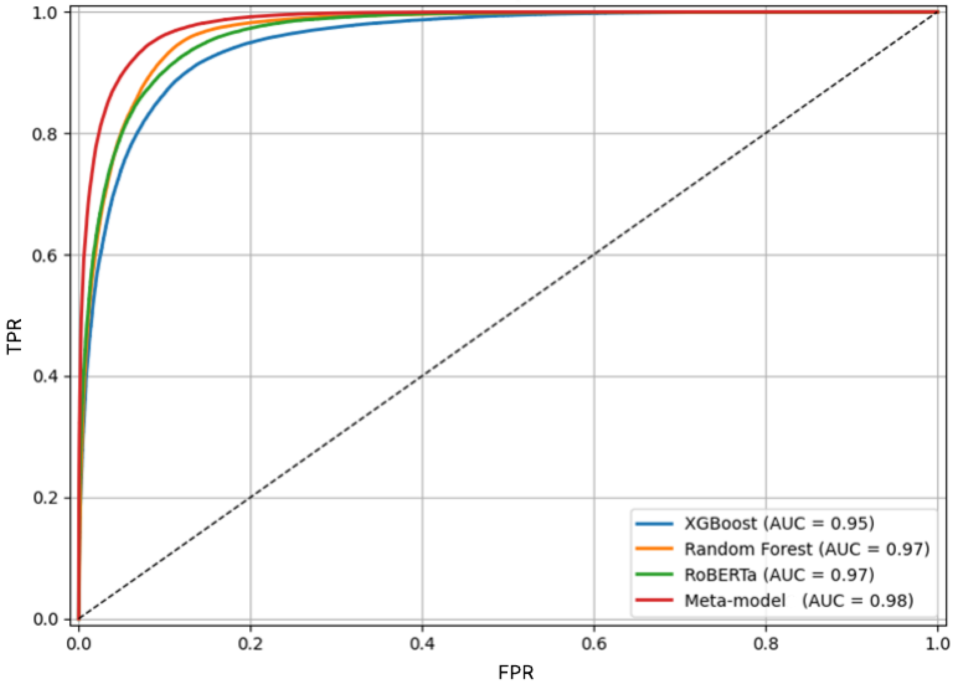
Furthermore, to evaluate the models’ performance, we used the Receiver Operating Characteristic (ROC) curve. As Google for Developers (2025) notes, the ROC curve graphically depicts the model’s performance across all thresholds. The AUC (area under the curve) value represents the probability that the model will correctly classify a positive example better than a negative one. A higher AUC indicates a better model.

Figure 10 presents the ROC curves. We see that the models achieve significant performance, with areas under the curve exceeding 0.95. The combined model achieves an area under the curve of 0.98, indicating a greater capacity to detect hate speech.

4.1.2. Emotional Tone Classification Models

For multiclass emotion classification, we evaluated the four models in the test data set. In

Table 8. Results of the models in emotional tone classification.

Metric	Label	Models
		RoBERTa	Random Forest	XGBoost	Combined
Precision	Anger	0.93	0.87	0.95	0.94
	Disgust	0.67	0.80	0.77	0.82
	Fear	0.43	0.86	0.80	0.88
	Joy	0.75	0.86	0.77	0.88
	Neutral	0.31	0.67	0.64	0.71
	Sadness	0.41	0.87	0.79	0.88
	Surprise	0.33	0.83	0.82	0.83
Recall	Anger	0.82	0.95	0.91	0.95
	Disgust	0.61	0.74	0.83	0.84
	Fear	0.86	0.67	0.76	0.79
	Joy	0.69	0.80	0.88	0.88
	Neutral	0.74	0.45	0.49	0.60
	Sadness	0.76	0.66	0.70	0.76
	Surprise	0.71	0.54	0.54	0.64
F1-Score	Anger	0.87	0.91	0.93	0.94
	Disgust	0.64	0.77	0.80	0.83
	Fear	0.57	0.75	0.78	0.83
	Joy	0.72	0.83	0.82	0.88
	Neutral	0.43	0.54	0.56	0.65
	Sadness	0.54	0.75	0.75	0.81
	Surprise	0.45	0.65	0.65	0.72

, we present the results of precision, recall and F1-Score for each of the seven emotions (i.e., anger, disgust, fear, joy, neutral, sadness, and surprise).

Regarding the accuracy metric, we obtain the following values:

• RoBERTa = 0.75;
• Random Forest = 0.85;
• XGBoost = 0.86;
• Combined = 0.90.

As shown in

Table 9. Confusion matrix of the models in emotional tone classification.

Model	Emotion	TP	TN	FP	FN
RoBERTa	Anger	92,133	81,506	6460	20,700
	Disgust	25,311	146,930	12,375	16,183
	Fear	3720	191,491	4992	596
	Joy	18,895	167,086	6176	8642
	Neutral	3626	187,686	1243	8244
	Sadness	5188	186,601	7375	1635
	Surprise	2087	193,655	4217	840
Random Forest	Anger	107,167	72,260	15,706	5666
	Disgust	30,731	151,496	7809	10,763
	Fear	2902	196,010	473	1414
	Joy	22,133	169,773	3489	5404
	Neutral	2208	194,849	1,081	2661
	Sadness	4525	193,296	680	2298
	Surprise	1579	197,556	316	1348
XGBoost	Anger	103,189	82,000	10,351	9644
	Disgust	34,239	148,954	10,351	7255
	Fear	3297	195,677	806	1019
	Joy	24,182	166,184	7078	3355
	Neutral	2388	194,590	1340	2481
	Sadness	4793	192,732	1244	2030
	Surprise	1585	197,531	341	1342
Combined	Anger	107,310	80,662	7304	5523
	Disgust	34,893	151,648	7657	6601
	Fear	3430	195,997	486	886
	Joy	24,260	170,022	3240	3277
	Neutral	2927	194,755	1175	1942
	Sadness	5159	193,262	714	1664
	Surprise	1868	197,496	376	1059

, we present the confusion matrices for each model, where true positives (TP), true negatives (TN), false positives (FP), and false negatives (FN) are grouped by emotion label.

Each colored curve in Figure 10 represents the performance of a different model (i.e., XGBoost, Random Forest, RoBERTa, and the meta-model), while the AUC values indicate its discriminatory power. The dashed diagonal line represents a reference random classifier. Curves closer to the upper left corner indicate better model performance in terms of true positive rate (TPR) versus false positive rate (FPR).

The results show that the combined model’s values surpass the evaluated metrics for most emotions. For the anger label, it achieves an accuracy of 0.94, a recall of 0.95, and an F1-score of 0.94, compared to the other individual models. For the disgust label, it achieves an accuracy of 0.82, a recall of 0.84, and an F1-score of 0.83. Regarding the fear label, it achieved an accuracy of 0.88 and an F1-score of 0.83, compared to the RoBERTa model, which had the lowest values with an accuracy of 0.43 and an F1-score of 0.57. Similarly, for the joy label, it achieves 0.88 in accuracy, recall, and F1-score. Although the value for the neutral label is lower, it still outperforms the other individual models. Finally, in the sadness label, it achieved an F1 score of 0.81 compared to 0.54 for RoBERTa. These results indicate that the combined model performs better across all labels.

We performed the procedure described above to analyze the statistical validity of the results. We calculated 95% confidence intervals for the accuracy metric using Wilson’s method for binomial proportions [51].

The intervals obtained for the evaluated models were: RoBERTa [0.7481, 0.7519], Random Forest [0.8484, 0.8516], XGBoost [0.8585, 0.8615], and the combined model [0.8987, 0.9013].

These results indicate that the confidence interval of the combined model remains clearly separated from those of the individual models, suggesting that the observed improvement is unlikely to be explained by random variation.

The confusion matrices presented in Table 9 support these results. The combined model shows higher values for true positives and true negatives while reducing false positives and false negatives in most emotions, suggesting a greater generalization capacity.

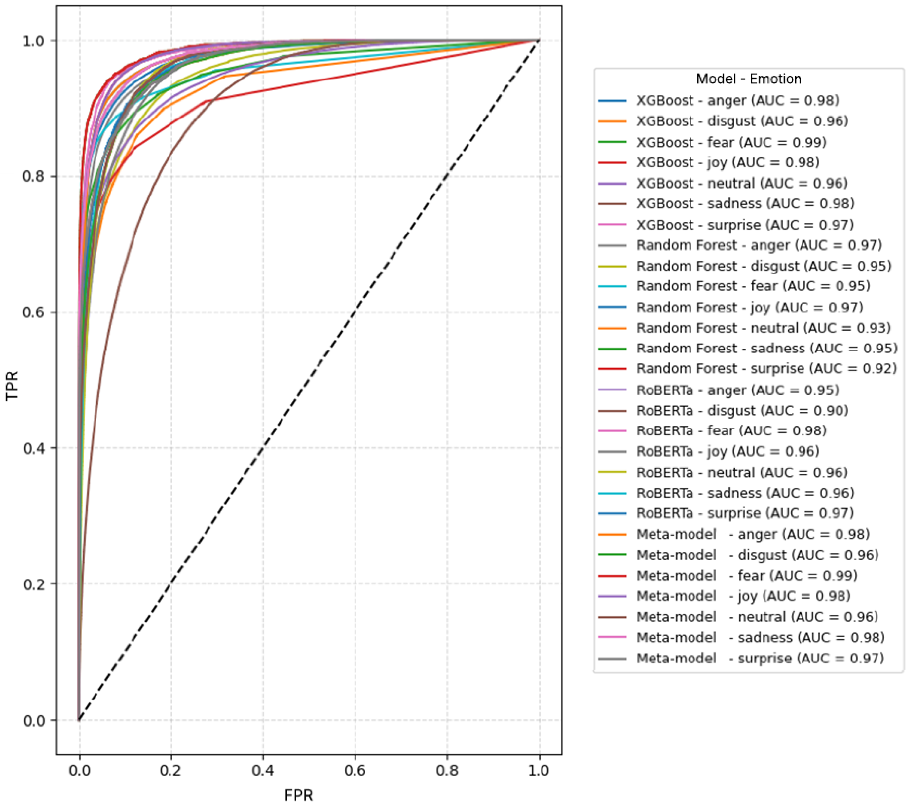
Figure 11 presents the ROC curves for each emotion. In this case, since it is a multi-class problem, we generated one curve per label. The combined model achieved curves closest to the ideal point, with higher AUC values for most emotions, notably anger (0.98), fear (0.99), joy (0.98), and sadness (0.98).

The multiple colored curves in Figure 11 represent the performance of the different models (i.e., XGBoost, Random Forest, RoBERTa, and the meta-model) for each emotional category. Each line corresponds to a specific emotion, and its AUC value reflects its classification performance. The dashed diagonal line indicates the performance of a random classifier, while curves closer to the upper-left corner indicate better performance.

4.1.3. REST API Performance Testing

We conducted performance tests to verify the RESTful API’s behavior under multiple concurrent users. We used Apache JMeter, a tool that allowed us to simulate user loads and generate real-time reports, measuring metrics such as average, minimum and maximum response times, standard deviation, error rate, and throughput. In each test, we configure a different number of users and a progressive increment period. The number of users increases by 100 to a maximum of 600.

Table 10. Performance test results of the REST API with Apache JMeter.

Scenario	# Samples	Average (ms)	Min (ms)	Max (ms)	Std. Dev.	% Error	Req/s	KB/s
100 users	100	27,651	1857	39,746	11,695.13	0.00%	1.27	0.74
200 users	200	52,630	2496	75,161	22,070.85	0.00%	1.33	0.76
300 users	300	49,008	346	78,085	26,791.32	13.00%	1.51	1.39
400 users	400	60,287	193	101,784	35,351.54	15.25%	1.52	1.47
500 users	500	42,688	190	91,543	37,188.87	35.00%	1.95	2.84
600 users	600	28,069	189	81,836	31,751.40	52.83%	2.33	4.45
Total	2100	42,997	189	101,784	16,303.78	28.19%	9.91	11.65

shows the details of the results obtained.

By exposing the API through an access tunnel with Ngrok, we identified bandwidth and traffic-control limitations that affected response times. With loads of 100 and 200 users, the API remained stable, with average response times of 27,651 ms and 52,630 ms, respectively, and no errors were recorded. Starting with 300 users, although the average response time decreased (49,008 ms), errors were reported (13%), reflecting an overload in the handling of concurrent requests. This trend intensified with 400 users (15.25% errors), and especially with 500 and 600 users, where errors reached 35% and 52.83%, respectively, demonstrating the API’s inability to process all requests.

The throughput increased from 1.27 req/s (100 users) to 2.33 req/s (600 users), indicating that the system attempted to process more requests, although not all were successful. Similarly, bandwidth consumption increased from 0.74 KB/s to 4.45 KB/s, highlighting the need for servers with greater power and capacity to support high concurrent loads.

The system was evaluated under controlled conditions as a proof-of-concept deployment scenario. While the API remained functionally stable up to approximately 200 concurrent users, the observed response times (27,651 ms for 100 users and 52,630 ms for 200 users) suggest that the current implementation does not meet the latency requirements of real-time or pre-moderation systems. Therefore, the proposed system should be interpreted as a proof of concept that validates the feasibility of the approach, rather than a production-ready solution.

Before introducing the BACON-AR framework, it is important to clarify that the performance metrics reported in the previous subsections correspond to the predictive capacity of the ensemble classifier itself. The BACON-AR framework does not modify the trained architecture or retrain the predictive models. Instead, it operates as a post hoc analytical layer applied to the probabilistic outputs generated by the ensemble.

Consequently, the purpose of the BACON-AR analysis is not to improve classification performance metrics such as accuracy or AUC but rather to analyze the calibration of predicted probabilities and determine an optimal decision threshold under asymmetric risk conditions. This distinction ensures that the predictive evaluation of the ensemble model and the risk-sensitive decision analysis performed by BACON-AR remain conceptually separated.

4.1.4. Analysis of the Bayesian Calibration and Optimal Design Under Asymmetric Risk (BACON-AR) Framework

This section analyzes the probabilistic output generated by the ensemble model using the BACON-AR framework. The objective is to evaluate the calibration of predicted probabilities and determine an optimal decision threshold under asymmetric risk conditions without modifying the underlying predictive model.

The BACON-AR framework, defined in Section 3.6.9, was applied to the validation data set to evaluate its empirical behavior under asymmetric decision costs. The ensemble model’s underlying architecture remained unchanged; only the probabilistic outputs were post-processed using Bayesian calibration and risk-based threshold optimization. In the experimental setup, asymmetric costs were defined as $C_{FN}=2C_{FP}$, reflecting the greater impact of false negatives on the target classification scenario.

The experimental configuration used to evaluate the BACON-AR framework is summarized in

Table 11. Experimental parameters and BACON-AR framework configuration.

Parameter	Description
data set	Balanced subset of 510,252 records
Training/validation split	80/20
Splitting strategy	Stratified by class (stratify = y)
Random seed	42 (reproducibility ensured)
Asymmetric cost	$C_{FN}=2C_{FP}$
Batch size	32
Number of repetitions	5 averaged runs
Calibration metric	ECE (Expected Calibration Error)
Risk metric	$R\left(t\right)$ with variable threshold $t\in [0,1]$

. While

Table 12. Comparative summary of the base model and BACON-AR framework with performance metrics, minimum risk, and optimal threshold.

Model	ECE (%)	AUC	Recall (%)	Precision (%)	Minimum Risk $\mathit{R}\left(\mathit{t}\right)$	Threshold t*
Ensemble (uncalibrated)	11.2	0.883	93.5	72.3	0.31	0.50
BACON-AR (calibrated)	11.2	0.883	93.5	72.3	0.24	0.43

presents the comparative results between the original ensemble classifier and the same model after applying the BACON-AR framework. The analysis focuses not only on traditional performance metrics (e.g., AUC, recall, and precision) but also on calibration behavior, minimum risk, and the decision threshold obtained via asymmetric risk minimization.

To avoid potential confusion, it is important to clarify that the metrics reported correspond to different stages and tasks within the proposed framework. The accuracy values close to 0.90 reflect the standalone performance of the base classifiers on specific tasks, such as hate speech detection and emotional tone classification. In contrast, the metrics reported in Table 12 correspond exclusively to the final ensemble output evaluated under the BACON-AR decision framework.

From an interpretative perspective, the results reported in Table 12 indicate that the ensemble classifier already produces reasonably calibrated probability estimates. Consequently, the Bayesian adjustment introduced by the BACON-AR procedure does not substantially modify the Expected Calibration Error.

It is important to distinguish between probability calibration and decision optimization. Although the Expected Calibration Error (ECE) remains approximately unchanged after BACON-AR is applied, this does not indicate a lack of contribution. Instead, BACON-AR operates at the decision level by selecting an operating threshold under asymmetric risk conditions.

BACON-AR does not modify the predictive architecture or improve its intrinsic classification performance. Instead, it operates as a post hoc decision layer over the ensemble probabilities. In the present results, its demonstrated contribution lies in selecting an operating threshold that minimizes total expected risk under asymmetric cost conditions. Therefore, the empirical effect of BACON-AR should be interpreted as cost-sensitive threshold optimization rather than as an improvement in predictive performance or a clear numerical gain in calibration.

The data used for this analysis came from the combined model trained with RoBERTa, Random Forest, and XGBoost. In the BACON-AR evaluation summarized in Table 12, the ensemble output achieved an AUC of 0.883, a recall of 93.5%, and a precision of 72.3%, while the framework was further analyzed from the perspective of calibration and asymmetric risk minimization.

Although the ensemble probabilities $P(y=1\mid x)$ were already reasonably calibrated according to the Expected Calibration Error reported in Table 11, the BACON-AR framework includes a Bayesian recalibration step as part of its structured post hoc decision procedure. In this context, the recalibration stage was applied to examine whether a lower-risk operating threshold could be obtained under asymmetric cost conditions rather than to correct a substantial calibration deficiency in the underlying ensemble model. This use of calibration remains consistent with the probabilistic interpretation of predicted confidence discussed in the calibration literature [39]. The general calibration formula is defined as

$$P_c(y=1\mid x)={\displaystyle \frac{P(y=1\mid x){\pi }_1}{P(y=1\mid x){\pi }_1+(1-P(y=1\mid x)){\pi }_0}},$$

(9)

where $P_c(y=1\mid x)$ represents the calibrated probability, $P(y=1\mid x)$ the original probability of the model, and ${\pi }_1$ and ${\pi }_0$ are the empirical proportions observed of the positive and negative classes. This adjustment aims to align the predicted probabilities with the observed empirical class proportions, following the calibration approaches described in the literature [16,40]. The calibration quality is subsequently evaluated through the Expected Calibration Error (ECE), which measures the discrepancy between the predicted confidence and the empirical accuracy across probability bins.

The computational development of the BACON-AR framework was implemented in Python, using NumPy and Pandas for probability calculations, calibration, and risk optimization. The mathematical procedure is summarized in Algorithm 4, which combines Bayesian calibration and the search for the optimal threshold $t^{*}$ that minimizes total risk $R\left(t\right)$.

Algorithm 4: BACON-AR: Bayesian Calibration and Optimal Threshold Selection under Asymmetric Risk.

The proposed BACON-AR procedure integrates Bayesian posterior recalibration with cost-sensitive decision optimization under asymmetric misclassification penalties. The calibration stage adjusts predicted probabilities according to empirical class priors, reducing prior-shift distortions and improving probabilistic interpretability.

Calibration quality is quantitatively assessed using the Expected Calibration Error (ECE), which measures the discrepancy between empirical accuracy and predicted confidence across probability bins.

The final decision rule is obtained by minimizing an asymmetric empirical risk function that explicitly incorporates differentiated costs for false negatives and false positives.

This formulation is in line with established principles in the evaluation and calibration theory of probabilistic models [52,53], ensuring the deployment of a statistically coherent and decision-aware model.

In this study, the Bayesian component of the BACON-AR framework refers specifically to posterior recalibration using empirical class priors estimated from the validation data, rather than to a fully parameterized Bayesian generative model with externally imposed prior distributions.

In practical terms, the ensemble probabilities are adjusted according to the proportions of the observed class before the asymmetric empirical risk is minimized. This clarification aligns the terminology of the framework with the mathematical apparatus actually implemented in the present study.

The Algorithm 4 summarizes the implementation of the BACON-AR framework. Before presenting the BACON-AR comparative results, Table 11 summarizes the experimental configuration used for calibration assessment, asymmetric-risk analysis, and threshold selection.

Starting with the ensemble probabilities, Bayesian calibration is applied, the expected calibration error (ECE) is calculated, and the asymmetric risk curve is obtained. The optimal threshold $t^{*}$ is selected as the point that minimizes $R\left(t\right)$, ensuring a decision consistent with the costs assigned to false negatives and false positives.

The parameters summarized in Table 11 describe the experimental configuration used to evaluate the BACON-AR framework.

It is important to note that the AUC, recall, and precision values reported in Table 12 correspond to the preserved predictive metrics of the underlying ensemble and are included to show that BACON-AR does not improve baseline predictive performance. By contrast, the quantities reported later in the sensitivity analysis correspond to threshold-dependent operating characteristics obtained under specific asymmetric cost ratios and should not be interpreted as directly comparable replacements for the values in Table 12.

As shown in Table 12, the global predictive metrics reported in this BACON-AR analysis, namely AUC, recall and precision, remained stable after the procedure was applied.

From a calibration perspective, the Expected Calibration Error (ECE) also remained numerically similar before and after the Bayesian adjustment, indicating that the ensemble classifier already produced reasonably calibrated probability estimates.

By identifying an optimal decision threshold, the framework allows the model to adapt its behavior to the relative impact of false negatives and false positives without altering its intrinsic predictive capacity.

This indicates that the framework does not alter the intrinsic predictive capability of the ensemble classifier but rather evaluates how probabilistic outputs can be translated into decisions under asymmetric cost conditions. Under the selected asymmetric cost configuration, adjusting the operating threshold from 0.50 to $t^{*}=0.43$ reduced the total risk without changing the reported predictive metrics. Therefore, the demonstrated contribution of BACON-AR in this study, should be interpreted as cost-sensitive threshold optimization on top of an existing classifier rather than as an improvement in predictive performance or a clear numerical gain in calibration.

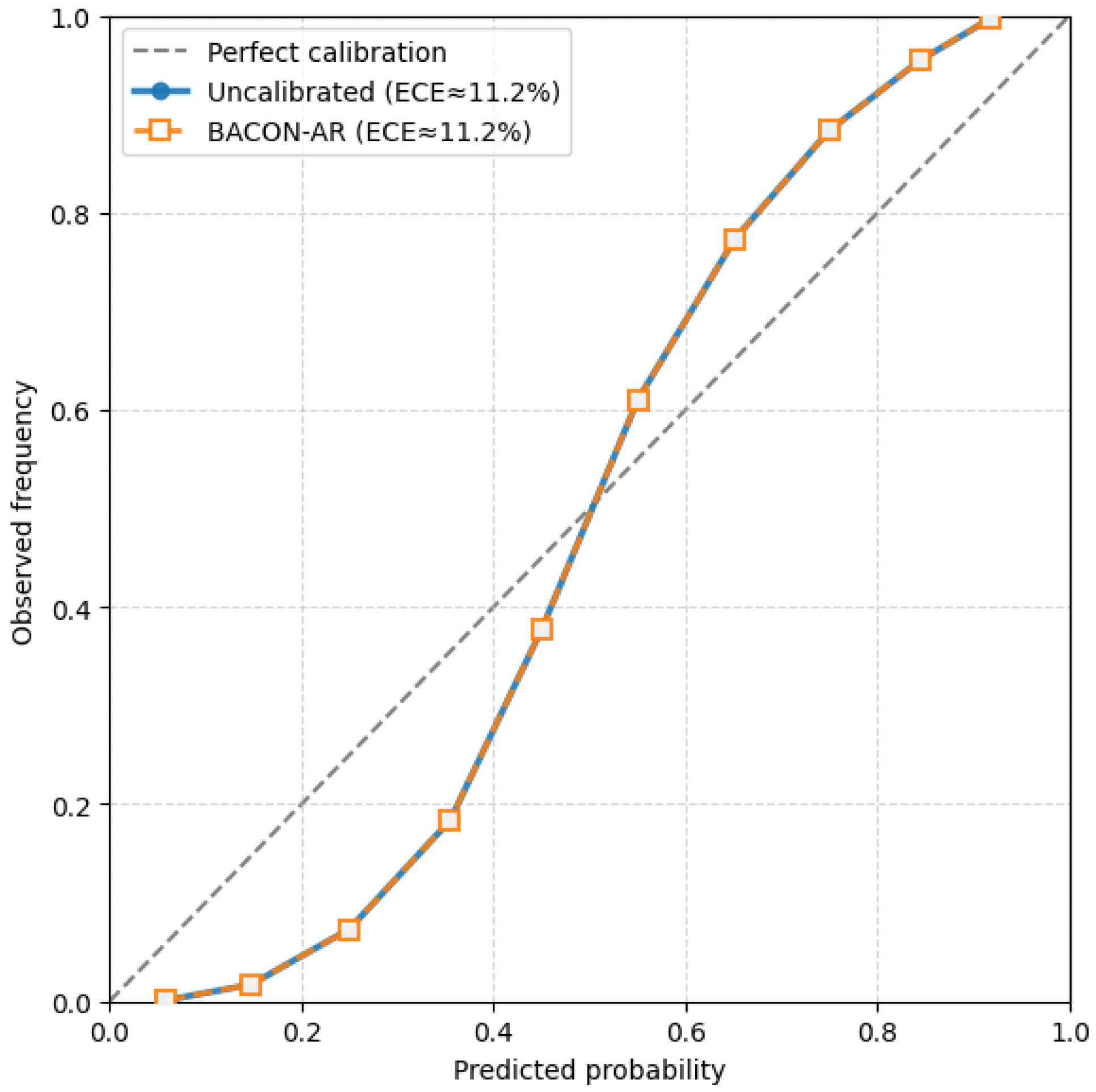
These findings were further examined through calibration analysis using the reliability diagrams shown in Figure 12. The dashed diagonal line represents perfect calibration, whereas the empirical curves correspond to the ensemble probabilities before and after applying the BACON-AR framework. The visual comparison indicates that the probabilistic estimates remain close to the ideal calibration trend, supporting the interpretation that BACON-AR preserves the ensemble output’s overall reliability structure while redefining the operating threshold under asymmetric cost conditions.

The comparison between the uncalibrated model and the output obtained after applying the BACON-AR framework indicates that the probabilistic estimates remained close to the ideal calibration line, following the interpretation commonly used in reliability analysis [54]. In practical terms, this result suggests that the framework preserved the overall calibration behavior of the model while redefining the decision threshold under asymmetric costs. The Expected Calibration Error remained approximately stable, which supports the interpretation that the proposed procedure did not distort the probabilistic structure of the ensemble predictions but instead provided a cost-sensitive decision adjustment on top of the existing classifier.

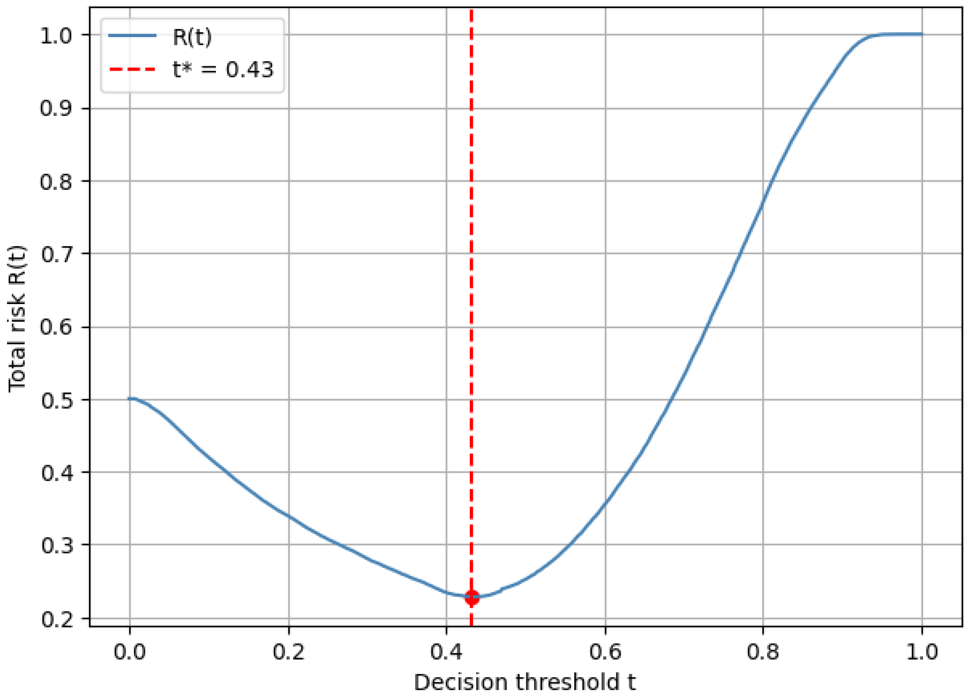
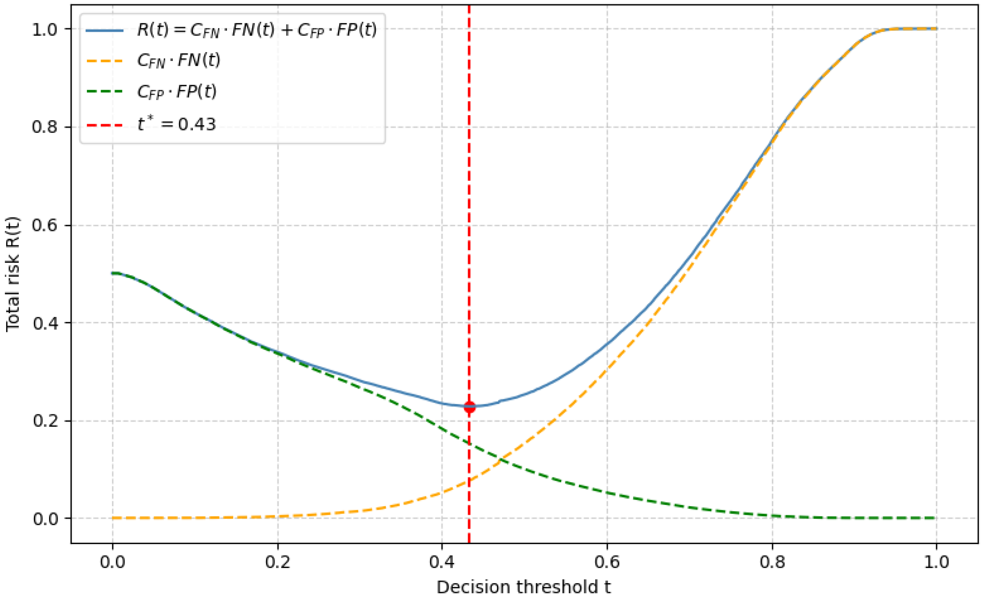
After examining the calibration behavior, the next step was to analyze how the asymmetric decision criterion changes the operating point of the classifier. Figure 13 presents the total risk function in the BACON-AR framework. This curve allows identifying the threshold that minimizes the expected risk when false negatives and false positives are assigned different costs. In this case, the minimum of the function is reached around $t^{*}\approx 0.43$, which indicates the most appropriate operating threshold in the selected asymmetric cost configuration.

In Figure 13, the red marker denotes the minimum-risk point of the curve, and the dashed red vertical line identifies the corresponding optimal threshold. Together, these visual elements indicate the operating condition in which the BACON-AR decision rule minimizes the expected total risk.

To provide a more detailed interpretation of the previous result, the total risk was decomposed into its two main components, namely, the contribution associated with false negatives and the contribution associated with false positives.

Figure 14 shows this decomposition and illustrates how both terms evolve as the decision threshold changes. This representation allows a clearer understanding of the trade-off induced by the asymmetric cost setting. As the threshold varies, one component decreases while the other increases, and the optimal point emerges at which the combined effect of both terms is minimal. In the figure, the red marker identifies that minimum-risk point, while the dashed red vertical line marks the threshold $t^{*}\approx 0.43$ at which the balance between false-negative and false-positive contributions becomes operationally preferable under the selected asymmetric cost configuration.

This decomposition reinforces the interpretation that the contribution of BACON-AR lies in selecting a cost-sensitive operating threshold under asymmetric conditions rather than changing the intrinsic predictive capacity of the underlying ensemble model.

To define the decision phase, the BACON-AR framework incorporates a total risk function expressed as

$$R\left(t\right)=C_{FN}P(y=1\mid x)I(P_c<t)+C_{FP}(1-P(y=1\mid x))I(P_c\ge t),$$

(10)

where $C_{FN}$ and $C_{FP}$ are the costs associated with false negatives and false positives, respectively, and $I(·)$ is the indicator function. The objective is to identify the threshold $t^{*}$ that minimizes the total risk:

$$t^{*}=arg\underset{t}{min}R\left(t\right).$$

(11)

This operating point is visually highlighted in Figure 13 and Figure 14 through the red marker and the dashed red vertical line.

The criterion was applied empirically to the validation data, establishing a cost relationship $C_{FN}=2C_{FP}$, where the cost of a false negative is considered twice that of a false positive, consistent with the nature of the problem and following the approach of [42]. The search for the minimum of the total risk function $R\left(t\right)$ determined an optimal value of $t^{*}=0.43$, which represents the equilibrium point between both types of errors in the selected asymmetric cost configuration [17].

This result highlights the primary contribution of the BACON-AR framework. Rather than modifying the predictive capacity of the ensemble classifier, the framework provides a structured analytical mechanism to translate probabilistic predictions into operational decisions under asymmetric cost conditions. By explicitly modeling the relative impact of false negatives and false positives, the decision threshold can be adjusted to reflect the priorities of the moderation scenario.

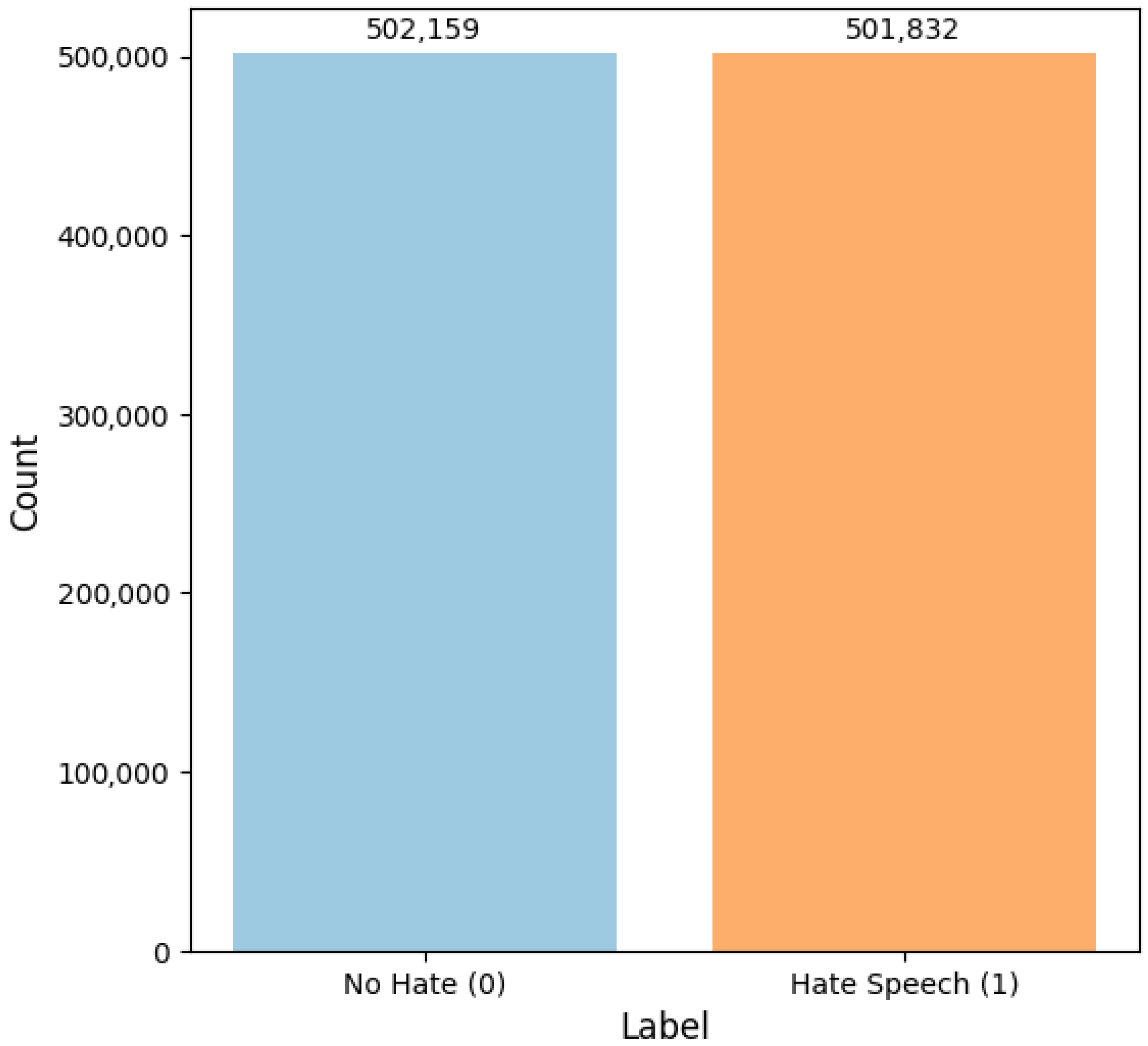
To evaluate whether the selected asymmetric cost ratio induces unstable decision behavior, a sensitivity analysis was performed by varying the relationship between false-negative and false-positive costs over the set $C_{FN}/C_{FP}\in \{1.0,1.5,2.0,2.5,3.0\}$, using the same balanced subset of 510,252 records.

Because BACON-AR operates as a post hoc decision layer, modifying this ratio does not retrain the underlying ensemble model; instead, it changes the operating threshold selected under the asymmetric decision criterion. Table 12, summarizes the resulting operating characteristics.

We include

Table 13. Threshold-dependent operating characteristics of BACON-AR under different $C_{FN}/C_{FP}$ ratios.

${\mathit{C}}_{\mathbf{FN}}/{\mathit{C}}_{\mathbf{FP}}$	Optimal Threshold ${\mathit{t}}^{*}$	FN	FP	Precision	Recall	F1-Score
1.0	0.50	7743	10,226	0.8089	0.8483	0.8281
1.5	0.45	4676	14,076	0.7671	0.9084	0.8317
2.0	0.43	3739	15,813	0.7494	0.9267	0.8269
2.5	0.41	2991	17,620	0.7316	0.9414	0.8234
3.0	0.40	2662	18,584	0.7224	0.9478	0.8199

to document how the BACON-AR operating point changes when the CFN/CFP ratio is varied under asymmetric cost conditions. Its purpose is not to demonstrate an improvement in the predictive performance of the classifier but to support the interpretation that the selected threshold $t^{*}$ = 0.43 follows from a sensitivity analysis of the decision rule and reflects the trade-off between false negatives and false positives in the adopted cost configuration.

Within the sensitivity analysis reported in Table 13, the selected configuration $CFN=2CFP$ yielded an optimal threshold of approximately $t^{*}=0.43$. At this operating point, the threshold-dependent operating characteristics were $FN=3739$, $FP=15,813$, precision $=0.7494$, recall $=0.9267$, and $F1=0.8269$. These values characterize the trade-off induced by the asymmetric decision rule. They should be interpreted as operating-point sensitivity results under a specific cost configuration, rather than as direct replacements for the ensemble-level metrics summarized earlier in Table 12.

As the relative cost assigned to false negatives increases, the optimal threshold decreases monotonically from 0.50 to 0.40. This shift reduces the number of false negatives from 7743 to 2662, at the expense of an increase in false positives from 10,226 to 18,584. In this sense, Table 13 should be interpreted as a sensitivity analysis of the operating point rather than as a second summary of the predictive performance of the ensemble classifier.

Additional bootstrap resampling confirmed the stability of this behavior, with low dispersion in threshold, recall, and F1-score across the evaluated ratios. For the selected configuration $C_{FN}=2C_{FP}$, the optimal threshold remained close to 0.43 in both repeated-run analysis ($0.4342\pm 0.0021$) and bootstrap estimation ($0.4311\pm 0.0035$), supporting its use as a balanced operating choice rather than as an arbitrarily fixed setting.

Using the same balanced subset of 510,252 records, the ensemble model maintained an AUC of 0.883 under the BACON-AR framework. These results indicate that BACON-AR can be used to select an operating threshold that is consistent with the selected asymmetric cost assumptions while preserving the predictive metrics of the underlying ensemble.

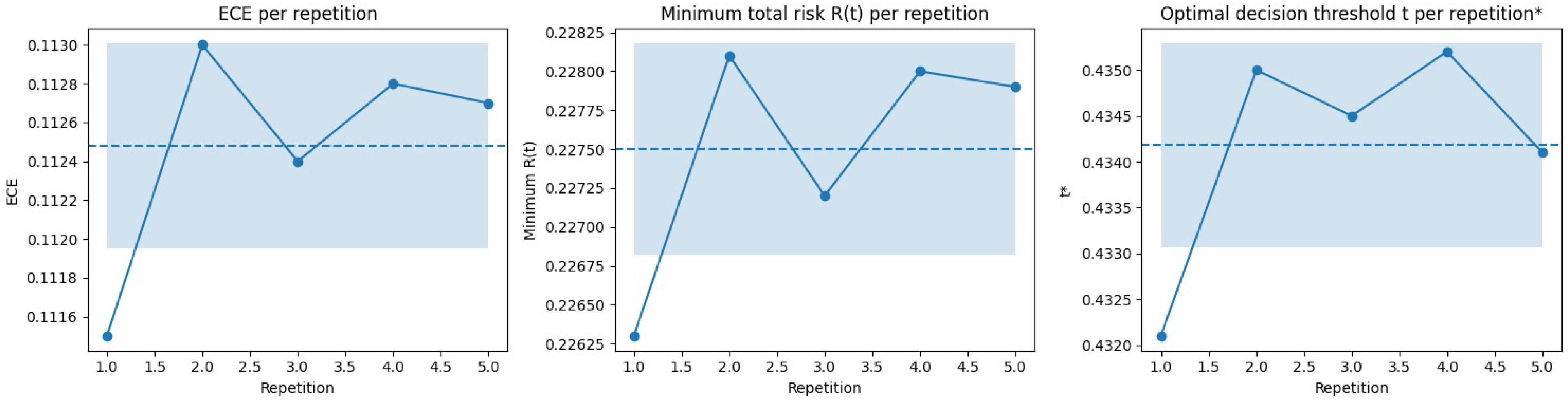
The statistical stability analysis of the BACON-AR framework showed consistent behavior in calibration and risk metrics. After five independent repetitions, the framework achieved an average ECE of $0.1125\pm 0.0010$, a minimum risk of $0.2275\pm 0.0012$, and a stable optimal threshold of $t^{*}=0.43\pm 0.002$, confirming reproducibility under small data perturbations.

Figure 15 summarizes the repeated-run stability analysis across five independent repetitions. In each subplot, the solid line represents the mean trajectory of the evaluated metric across runs, while the shaded band represents the variability associated with the corresponding standard deviation. The three panels show the behavior of the Expected Calibration Error, the minimum total risk, and the optimal threshold, respectively.

These results indicate that the BACON-AR framework maintained stable calibration and decision behavior under small variations in the validation data, which is desirable in operational moderation systems where decision policies must remain consistent across changing samples.

5. Discussion

The results demonstrate that the developed models can be efficiently integrated into web applications via a RESTful API, enabling requests to be sent from the interface to the server and responses to be received in real time. This architectural design promotes scalability and interoperability in real-world environments because it does not depend on any particular technology for its consumption. Thus, the system can be easily adapted to different platforms or services, expanding its practical applicability.

These findings are consistent with previous research highlighting the usefulness of lightweight, decoupled architectures for implementing artificial intelligence systems in production, as they reduce maintenance complexity and improve the model’s ability to be continuously updated.

According to the study hypothesis, the combined model outperformed individual models in the standard predictive evaluation setting, achieving accuracy values of 0.93 for hate speech detection and 0.90 for emotion classification. Furthermore, the F1-score and AUC metrics exceeded 0.95 in several cases, indicating strong predictive performance and a favorable generalization profile across the evaluated tasks.

This behavior supports the idea that ensemble models are robust for complex tasks such as identifying hostility and emotional tone in texts, as also noted by Al-Hashedi et al. [54] in the recent study titled Detection of Cyberbullying-Based on Emotion.

In this context, the results of this work reinforce the evidence that combining classifiers can increase the stability of NLP-based systems and provide stronger predictive behavior than individual models under the experimental conditions evaluated.

In addition to the predictive gains obtained through the ensemble architecture, it is important to emphasize the complementary role played by the BACON-AR framework within the decision pipeline. Unlike the ensemble classifier, which is responsible for generating probabilistic predictions, BACON-AR operates as a post-processing decision layer that evaluates those probabilities under asymmetric cost conditions. In this sense, the framework does not modify the internal parameters of the predictive model; instead, it analyzes the confidence values produced by the ensemble to determine a threshold that minimizes the expected operational risk.

This distinction is particularly relevant in socially sensitive tasks such as hate speech detection, where the practical consequences of classification errors may differ substantially. By explicitly incorporating asymmetric costs into the decision rule, BACON-AR uses ensemble probabilities to identify an operating threshold that reflects the relative operational importance of false positives and false negatives.

The results of the mathematical analysis show that the BACON-AR framework identifies a cost-sensitive operating threshold at $t^{*}=0.43$. This value corresponds to the point at which the total risk function minimizes the combined contribution of both types of errors in the selected asymmetric cost configuration. These findings support the interpretation that BACON-AR functions as a cost-sensitive threshold optimization layer by aligning the final classification rule with the relative operational cost of false positives and false negatives. Under the selected asymmetric thresholding policy, BACON-AR identified a lower-risk operating threshold while preserving the reported predictive metrics of the underlying ensemble. This result is consistent with previous work showing that asymmetric cost modeling can support operating-threshold selection in imbalanced classification settings.

This interpretation is also consistent with prior work showing that calibration-aware and cost-sensitive decision rules can support more stable operating policies in applied classification settings. In this study, the contribution of BACON-AR should therefore be understood as providing a structured mathematical mechanism for cost-sensitive threshold selection rather than as an improvement in the intrinsic predictive performance or calibration of the underlying classifier.

Beyond the specific application addressed in this study, the BACON-AR framework also illustrates a broader methodological contribution for machine learning systems operating in environments where classification errors have unequal consequences. In such contexts, predictive accuracy alone is often insufficient to guarantee reliable decision-making. Instead, it becomes necessary to combine probabilistic modeling with explicit risk-aware decision rules.

The proposed framework contributes to this objective by integrating Bayesian calibration and asymmetric risk optimization into a coherent post-processing strategy that can be applied to the probabilistic outputs of different predictive models. This characteristic makes BACON-AR adaptable to other domains in which cost-sensitive threshold selection is required, including content moderation systems, automated monitoring tools, and other decision-support applications based on natural language processing. Consequently, the framework provides a structured post-processing strategy for cost-sensitive threshold selection based on the probabilistic outputs of the underlying classifier, without implying an improvement in its intrinsic predictive performance or calibration.

Despite the robust predictive performance achieved by the proposed hybrid architecture, several methodological limitations must be acknowledged. As with many natural language processing systems, the model may struggle to interpret sarcastic or ironic expressions, where the literal meaning of the text differs from the communicative intent. Similarly, the presence of slang, informal language, and rapidly evolving expressions, typical of social networks, can affect the model’s ability to generalize across different communicative contexts.

Another limitation concerns the reliance on the data sets used for training. Although the integrated corpus contains over a million records, the distribution of patterns and linguistic expressions may still reflect biases in the original sources, potentially influencing the model’s performance when applied to other domains or platforms.

From an implementation perspective, technical limitations were also observed during deployment testing. During experiments conducted on a prototype server hosted on Google Colab and exposed through an Ngrok tunnel, latency issues and occasional failures were recorded in concurrent scenarios with over 300 simulated users. These results indicate that the observed limitations are primarily associated with the experimental deployment infrastructure, rather than the predictive models themselves.

This observation also aligns with the recommendations of [47], who emphasize the importance of controlled, reproducible environments to ensure performance stability in artificial intelligence systems.

From a practical perspective, one of the system’s main advantages is its potential to serve as a verification point before content is published on digital platforms. This would allow for blocking hate speech and classifying its emotional tone before it is publicly viewed, thus reducing the negative impact on victims and contributing to the creation of safer digital spaces.

Furthermore, this type of preventive integration aligns with the ethical principles of artificial intelligence outlined by [55], which emphasize calibrated models that ensure equitable and socially responsible decisions.

Among the methodological limitations, it is acknowledged that the training data are in English, which limits the models’ ability to generate predictions in other languages natively. Although machine translation models were incorporated, they do not always accurately capture terms, nuances, and expressions, leading to errors in some predictions.

Furthermore, it is important to consider that translation errors can introduce “translation noise,” which can affect the preservation of the text’s semantic meaning and emotional tone. This is especially relevant in the detection of hate speech, where subtle linguistic cues, implicit offensiveness, or culture-dependent expressions can be altered during translation.

As a result, the performance indicators presented in this study reflect the combined effect of both the translation process and the classification model. However, the specific impact of translation quality on classification accuracy was not independently assessed. Future work could include a comparative analysis of the original and translated texts to quantify how translation errors influence the model’s performance.

This difficulty has also been reported in previous work on multilingual natural language processing, where cultural and contextual differences influence the semantic interpretation of texts. Expanding the linguistic scope, therefore, represents a relevant methodological challenge in improving the generalizability of the models.

Regarding future research lines, it is pertinent to expand training with multilingual corpora specific to the local sociocultural context. This would improve the detection of emotional nuances in different languages.

Similarly, it would be beneficial to explore the use of multimodal models that integrate text, audio, and image to more comprehensively identify hostility and emotions, as well as to apply explainable learning techniques to improve the transparency and traceability of model decisions.

Finally, the main validation of this study lies in the practical integration of Bayesian decision theory and probabilistic calibration for classification problems with unequal costs. The BACON-AR framework provides a solid theoretical foundation, a reproducible mathematical formulation, and verifiable empirical validation, positioning it as a reliable alternative for automated decision-making with explicit risk control.

6. Conclusions

In this study, we address the problem of hate speech on social networks, a phenomenon that frequently affects vulnerable groups and may manifest in forms such as online misogyny. We propose a classification model that integrates emotional tone analysis with the detection of explicit hostility, offering a more precise and sensitive tool to identify harmful discourse.

The results demonstrate that the combined approach consistently outperforms individual models, achieving accuracy and F1 Scores of 0.93 for hate speech detection and 0.90 for emotional tone classification.

Furthermore, the analysis using confusion matrices and ROC curves confirmed the system’s robustness, with AUC values of up to 0.98 for basic emotion detection, demonstrating a suitable balance between sensitivity and specificity in multiclass scenarios.

The primary advancement of this work lies in integrating Natural Language Processing (NLP) and machine learning techniques within a hybrid approach that incorporates emotional tone analysis as an essential complement for identifying hostile speech.

This advancement not only enhances the ability of moderation systems to distinguish between ironic, ambiguous, or discriminatory messages but also promotes the creation of safer, more equitable digital environments.

Practical implementation using a RESTful API and its validation in a web environment demonstrated the technical feasibility of the proposal in real-world scenarios, consolidating a scalable and lightweight architecture adaptable to different platforms.

From a mathematical perspective, the BACON-AR framework demonstrated that combining Bayesian calibration with asymmetric risk-based decision-making provides a cost-aware decision layer atop the ensemble predictions. The total risk function reached its minimum at $t^{*}=0.43$, corresponding to the operating threshold that minimized the combined contribution of false positives and false negatives when the cost of false negatives was set to twice that of false positives. In this asymmetric thresholding configuration, the framework identified a lower-risk operating threshold while preserving the predictive metrics reported by the underlying classifier. In this sense, BACON-AR contributes methodologically by connecting Bayesian decision theory with probabilistic calibration in operational classification settings.

Regarding the study’s limitations, the system’s performance decreased under high concurrency, leading to significant error rates when more than 300 users accessed it simultaneously. This finding highlights the need to migrate to more robust distributed infrastructures that maintain availability and performance in production environments.

Furthermore, the reliance on data collected on specific platforms limits the model’s ability to generalize across different cultural and linguistic contexts, posing a challenge for its large-scale application.

Looking ahead, the proposal is to delve deeper into optimization strategies for large-scale systems while also exploring self-supervised and multilingual learning techniques that expand the model’s capacity to adapt to diverse digital communities.

Similarly, it is pertinent to investigate the use of multimodal models that integrate text, audio, and image to detect hostility and emotions more thoroughly and to apply explainable learning methodologies that improve the transparency and traceability of decisions. The aim is to move towards more inclusive, scalable, and reliable detection systems that effectively prevent hate speech and promote respectful, safe digital spaces for women and other vulnerable groups.

Together, the BACON-AR framework and the proposed web architecture provide a coherent methodological and practical contribution toward automated systems for socially sensitive language analysis. In summary, this work integrates predictive modeling, calibrated cost-aware decision-making, and deployment considerations into a unified proposal for the detection of hate speech and emotion classification.

In summary, this work offers a comprehensive proposal that combines technical soundness, mathematical rigor, and an ethical vision for the use of artificial intelligence.

7. Future Work

In future work, we first propose to construct a parallel corpus that includes Spanish and its regional variants to capture the linguistic diversity of Latin American digital communities. Current models trained in English should be expanded to support multilingual capabilities and dialect-aware representations that preserve local expressions and culturally specific manifestations of gender-based hostility. Such an extension would directly address the machine translation limitations identified during the API validation stage.

Second, the performance degradation observed under high-concurrency loads demands architectural improvements. Migrating the system from the current prototype to a distributed cloud infrastructure with auto-scaling capabilities would ensure production-level reliability. Containerization strategies and asynchronous request processing could significantly reduce latency while maintaining prediction quality under real-world traffic patterns. This infrastructure upgrade would enable the system to function as a viable pre-moderation tool for social platforms.

Third, extending the system beyond text-based analysis represents a natural progression. Online hate speech increasingly appears in multimodal formats, such as memes and images, that can evade conventional filters. Developing a multimodal ensemble that incorporates visual features would address this limitation. The stacking architecture validated in this study provides a flexible foundation for integrating additional modalities while preserving the emotional tone classification component.