Evaluating Reconstruction-Based and Proximity-Based Methods: A Four-Way Comparison (AE, LSTM-AE, OCSVM, IF) in SCADA Anomaly Detection Under Inverted Imbalance

Abstract

This article investigates and compares four unsupervised anomaly detection algorithms: the Autoencoder (AE), LSTM-Autoencoder (LSTM-AE), One-Class SVM (OCSVM), and the Isolation Forest (IF). The analysis focuses on SCADA telemetry data from an urban wind turbine, characterized by a unique case of extreme inverted class imbalance, where operational anomalies constitute 75.7% of the records. The AE model, trained exclusively on the rare normal state, achieved the best overall performance (AUC 0.9667), maintaining balanced and high classification effectiveness for both classes (Recall Normal ≈ 95%, Recall Anomaly ≈ 88.5%; Macro F1-Score 0.8962). In contrast, the IF model, despite a strong discriminative ability (AUC 0.8616), exhibited a complete inability to correctly recognize the normal class (Recall Normal 0.00) when using the optimal F1-score threshold. This performance degradation was a direct consequence of the necessity to apply a classification threshold imposed by the statistical fraction of the anomaly-dominated dataset. These results empirically demonstrate the methodological superiority of the reconstruction-based approach (AE) in constructing a stable decision boundary independent of the statistically dominant class. The study provides quantitative guidelines for the selection and calibration of algorithms in PHM diagnostic systems where states deviating from the operational norm constitute the majority.

1. Introduction

Operational security, energy efficiency, and predictive optimization of electrical power systems, especially distributed renewable energy sources, constitute a key area of contemporary research in engineering and critical infrastructure management [1]. SCADA (Supervisory Control and Data Acquisition) systems form a fundamental operational layer, generating continuous streams of telemetric data that serve as ideal material for advanced Predictive Health Management (PHM) applications [1]. The core goal of PHM is to provide comprehensive solutions for maintaining system “health,” directly translating into reduced operational costs (O&M) and preventing catastrophic failures, particularly under the harsh operating conditions of Wind Turbines (WT) [1].

However, deploying advanced algorithms in SCADA environments involves several challenges, including lower computational power of end devices and the necessity for integration with unique communication protocols [2]. This demands not only high diagnostic accuracy but, above all, the stability and efficiency of the model’s operation in real-time.

1.1. Evolution of Anomaly Detection and Data Challenges in Wind Turbines

Traditional anomaly detection focuses on identifying rare events (e.g., mechanical failures) within a dataset dominated by normal data. Industrial data is generally characterized by non-linearity, high dimensionality, and a fundamental lack of sufficient failure data [3]. PHM has evolved from traditional statistical and physics-based methods to approaches reliant on Machine Learning (ML) and Deep Learning (DL), which offer powerful capabilities for automatic feature extraction from raw SCADA data [4].

Deep Learning approaches, such as Autoencoders (AE) and their sequential counterparts like LSTM-Autoencoders (LSTM-AE), are gaining importance due to their ability to learn complex, latent representations (the “manifold”) of the normal operational state. This is particularly valuable in industrial settings where labeled anomaly data is scarce or unreliable [5].

The challenges in wind turbine PHM systems are multifaceted, encompassing not only modeling techniques but also the data characteristics themselves [3]. The most significant of these challenges, along with their consequences for diagnostic modeling, are summarized in

Table 1. Key Challenges in Predictive Diagnostics of SCADA Systems.

Challenge Area	Problem Characteristics	Impact on Diagnostic Modeling	Literature Reference
Data Quality and Quantity	Scarcity of failure data (rare labels), massive amounts of normal data, need for synthetic data generation	Hinders training of supervised models, requires One-Class Classification (OCC) and Transfer Learning approaches	[6]
Uncertainty and Variability	Difficulty in precise RUL (Remaining Useful Life) prediction, high non-linearity and variability of operational conditions	Requires models with uncertainty quantification and robust decision thresholds	[1]
SCADA Constraints	Limited computational power and specificity of industrial protocols (e.g., IEC 60870-5-104)	Requires models that are fast in inference and stable, with a low rate of False Positives	[2]
Class Imbalance	Traditional (rare anomaly) or Inverted (dominant anomaly)	Forces verification of fundamental assumption that anomaly is a rare outlier, leading to severe threshold instability in algorithms like IF	This Study

.

1.2. The Research Context: Extreme Inverted Class Imbalance Problem

This work focuses on the specific context of an urban wind turbine in São Paulo, where operational states other than the optimal status, “Normal. Run with energy generation” (e.g., Low Windspeed, Braking, Waiting), are classified as operational anomalies from the perspective of maximizing energy production.

The analyzed dataset [7] is characterized by a unique and extreme case where these operational anomalies constitute the majority, amounting to approximately 75.7% of all recorded entries. The “Normal. Run” state is, in this context, the minority (approximately 24.3%). This phenomenon is referred to in this article as inverted class imbalance.

This inversion poses a unique methodological challenge, questioning the fundamental assumptions of many unsupervised algorithms, which traditionally assume that an anomaly is a rare outlier [8]. Specifically, algorithms based on proximity (like Isolation Forest, IF, and One-Class SVM, OCSVM) may struggle when the minority class (Normality), which the method must accurately model, is traditionally assumed to be the anomaly class which the method is designed to isolate, leading to critical instability in the classification threshold (threshold instability). In contrast, reconstruction-based models (AE and LSTM-AE), trained exclusively on the rare Normal state, must demonstrate the ability to learn a narrow space of normality for stable thresholding.

1.3. Methodological Challenge and Research Aim

The main goal of this article is to conduct a rigorous, empirical, and quantitative comparison of the performance and methodological stability of four distinct unsupervised models—Autoencoder, LSTM-Autoencoder, One-Class SVM (OCSVM), and Isolation Forest (IF)—in the task of binary operational anomaly detection under conditions of an extremely anomaly-dominated SCADA dataset.

Specifically, the analysis focuses on three critical questions:

• Reconstruction vs. Proximity: How do the methodologies of learning the normality manifold (AE, LSTM-AE) compare to methods based on boundary separation (OCSVM) or rapid isolation (IF) under inverted imbalance?
• Temporal Modeling: What is the specific impact of introducing sequential dependency modeling (LSTM-AE) on overall discriminative ability, Area Under the Curve (AUC) and classification stability compared to the static AE? (This directly addresses potential reviewer feedback.)
• Threshold Stability: What is the critical impact of the thresholding strategy—statistical fraction (which severely impacts IF) vs. reconstruction error statistics (AE, LSTM-AE)—on the final classification balance (Macro F1-Score) when the anomaly class is the majority?

These results provide quantitative guidelines for the selection and calibration of algorithms in PHM systems facing similar, atypical data dynamics, where states of non-normal operation constitute the majority of the system’s runtime.

2. Related Work

This section situates the research objectives within the context of existing scientific knowledge concerning Predictive Health Management in SCADA systems. The review begins with a discussion of anomaly detection architectures in wind turbines, subsequently moving to a detailed methodological analysis of One-Class Classification. Particular emphasis is placed on verifying the design assumptions of the four main algorithms (AE, LSTM-AE, OCSVM, IF) and on substantiating the research novelty, which stems from the empirical testing of their stability in the unique scenario of inverted class imbalance.

2.1. Anomaly Detection Architectures in SCADA Systems: The PHM Context

Diagnosis and prognosis within SCADA systems for renewable energy sources, including wind turbines, have evolved from physics-based models to advanced data-driven approaches [1,9]. Physics-based models, while potentially accurate, are difficult to apply in dynamic and non-linear systems without simplification and require complex validation [1].

In response to the sheer volume and high dimensionality of SCADA data, Deep Learning methods—such as Convolutional Neural Networks (CNNs), Recurrent Neural Networks (RNNs), and Autoencoders—have gained popularity due to their powerful capability for automatic feature extraction from raw telemetric data [4,10]. Compared to classical Machine Learning algorithms, such as Random Forest (RF) or Support Vector Machines (SVM), DL models often achieve comparable or superior accuracy, but at the cost of greater training complexity and a requirement for large datasets [6].

Challenges in PHM often involve managing model uncertainty, the need for effective data augmentation, and handling system non-linearity [3]. For SCADA systems, deployment efficiency is a particularly crucial factor. Although industrial infrastructure requires high reliability, its limited computational power necessitates prioritizing the stability and speed of inference [2]. For this reason, a model that can guarantee a stable decision boundary and high evaluation speed is preferred in engineering applications.

2.2. Comparative Analysis of One-Class Classification Algorithms: Reconstruction vs. Proximity

In the context of anomaly detection, particularly when data is imbalanced or labels for the anomaly class are scarce, unsupervised learning or One-Class Classification methods are employed [11]. OCC approaches train a model exclusively on examples of the normal class (traditionally the majority) to effectively identify deviations as anomalies [11]. The models compared in this study can be grouped into two main methodological categories: Reconstruction-Based (AE, LSTM-AE) and Proximity/Boundary-Based (IF, OCSVM).

2.2.1. Reconstruction-Based Methods: AE and Temporal LSTM-AE

Autoencoders (AEs) operate on the logic of learning a compact, low-dimensional representation (encoding) of the training data by exclusively training on examples of the Normal class. The key detection mechanism is the Reconstruction Error (Mean Squared Error—MSE). If a new record does not fit the learned normality space, the reconstruction error is high, signaling an anomaly [5].

The advantage of AE architectures is the stability of their thresholding, which is calibrated based on the reconstruction error statistics of the pure Normal subset (e.g., the 95% MSE quantile). This threshold is internally linked to the learned normality, making it independent of the anomaly’s fraction in the overall dataset.

LSTM-Autoencoders: By incorporating Recurrent Neural Networks (RNNs), the LSTM-AE extends the AE approach to time series data, learning the normal sequence dependency. This is crucial in SCADA data where anomalies are often defined by a breakdown in temporal patterns rather than just static feature values [12]. The use of LSTM-AE directly addresses the need to evaluate the influence of temporal modeling on detection efficacy in the presence of inverted imbalance.

2.2.2. Proximity/Boundary-Based Methods: OCSVM and Isolation Forest

One-Class SVM: This classic boundary-based OCC method aims to find a hyperplane that best separates the training data (Normality) from the origin, thereby enclosing the normal data space [11]. OCSVM uses a decision function whose values define the distance to this boundary. Its performance depends heavily on the chosen kernel and the containment parameter (ν).

Isolation Forest: IF is a tree-based ensemble method whose fundamental logic relies on the assumption that outliers are rare and differ significantly from the majority of the data, allowing them to be isolated using a small number of random hyperplane splits [11,13].

The key weakness for both OCSVM and IF in this work emerges during threshold binarization. In the inverted imbalance scenario (where normality is the minority, ≈24.3%), any classification threshold that aims to accurately capture the dominant anomaly fraction (75.7%) inherently risks collapsing the normal class boundary. While IF is typically robust, our research empirically tests multiple thresholding strategies, including the standard contamination parameter equivalent and an Optimal F1-Score search. The Failure Mode observed across both Isolation Forest and LSTM-Autoencoder in this context—where the model maintains strong discriminative ability (AUC 0.8616 for IF), but the decision boundary severely compromises the minority class (e.g., Recall Normal ≈ 0.00)—highlights the fundamental inadequacy of relying on score distribution statistics or heuristics for classification when the anomaly is statistically dominant. The methodological challenge necessitated a detailed ablation study of the Isolation Forest model across multiple thresholding strategies (fraction-matched, contamination-matched, and optimal F1-Score).

Table 2. Methodological Comparison of OCC Algorithms in Temporal and Imbalance Contexts.

Methodological Feature	Autoencoder	LSTM-Autoencoder	One-Class SVM	Isolation Forest
Learning Paradigm	Reconstruction-Based: Low-Dimensional Representation Learning (Manifold)	Temporal Reconstruction: Sequential Normality Learning (Temporal Manifold)	Boundary Separation: Finding an optimal boundary separating data from the origin	Isolation-Based: Isolating extreme points (Outlier Detection)
Temporal Modeling	No (Static)	Yes (Sequences/Time)	No (Static)	No (Static)
Training (Input)	Exclusively on Normal Data (Minority Class)	Exclusively on Normal Sequences	Exclusively on Normal Data (Minority Class)	Entire Dataset (Normality + Anomaly)
Detection Mechanism	Reconstruction Error (MSE)	Sequence Reconstruction Error (Sequence MSE)	Decision Function (Distance from Boundary)	Ease of Isolation (Score Samples) using random splits
Fundamental Assumption	Normality is cohesive and reproducible (narrow space)	Normal sequential pattern is reproducible	Normality can be enclosed by a single boundary	Anomaly is rare (minority)
Thresholding Strategy	Based on MSE Quantile (e.g., 95%), calibrated on the pure minority	Based on Sequence Error Quantile, calibrated on the pure minority	Based on Decision Function Quantile (e.g., 5%), calibrated on the pure minority	Typically based on dataset fraction or heuristics; unstable with dominant anomaly

summarizes the key methodological differences that determine the models’ performance under inverted imbalance conditions.

2.3. Class Imbalance Challenges in PHM Context and “Inverted Imbalance”

Traditionally, the imbalanced data problem in PHM of industrial systems, such as wind turbines, focuses on the scarcity of failure data [6]. The rarity of faults means that supervised models are unable to effectively learn the feature space of anomalies. To address this, methods for generating synthetic data or oversampling/undersampling techniques are employed [14]. There are also established theoretical frameworks that analyze the general phenomenon of Class Imbalance (CI) in anomaly detection [8]. These frameworks often incorporate concepts like cost-sensitive learning or re-sampling techniques to mitigate the bias towards the majority class [14]. However, these traditional methods primarily address the scenario where the anomaly is the minority. In our inverted scenario, the traditional concept of cost is implicitly tested: the cost of misclassifying the Normal state (minority) becomes extremely high. We intentionally avoid common imbalance mitigation techniques (like re-sampling) to directly test the inherent stability of the algorithms when facing this dominant anomaly.

In the inverted class imbalance scenario, where the anomaly class (e.g., Low Windspeed, Waiting states) constitutes a clear majority (75.7%), and the normal state is the minority (24.3%), the One-Class Classification paradigm becomes the only viable solution. Instead of learning the dominant class, the Reconstruction-Based models (AE, LSTM-AE) are intentionally trained exclusively on the minority class (Normality 0). The purpose of this is to construct a tight and precise boundary around “normality,” which can then be used for discrimination.

The Failure Mode observed for the Isolation Forest model in this context—resulting from the necessity to impose a threshold consistent with the dataset statistics—empirically proves the fundamental inadequacy of using fraction-based thresholding in the case of inverted imbalance, despite the model’s good ability to rank the anomaly scores (AUC), which is a key conclusion of this research.

2.4. Dataset Context, Novelty, and Research Hypotheses

The research is based on a publicly available SCADA dataset from an urban wind turbine in São Paulo [7]. This context is essential for the credibility of PHM research, as SCADA data are characterized by high operational variability. While limited to a single case study, the research goal is methodological: to provide an empirical basis for selecting the most robust algorithmic paradigm (reconstruction vs. isolation) for any system facing similar inverted imbalance challenges, a problem common in systems where suboptimal operation is frequent.

In contrast to established benchmarks, such as the “CARE to Compare” dataset [15], which assume that training data is dominated by normal behavior, the uniqueness of this research lies in deliberately exploiting the naturally occurring extreme dominance of operationally anomalous states (75.7%) to conduct a critical methodological test.

Prior literature [16,17,18,19,20], verified in the context of this specific dataset [7], has not established its interpretation as an extreme case of inverted imbalance. Consequently, the novelty of this research lies not in the data itself, but in the methodological challenge it imposes: the empirical testing of whether four fundamental anomaly detection paradigms (Reconstruction-Based, Temporal Reconstruction-Based, Boundary-Based, and Isolation-Based) are able to maintain the stability of the decision boundary in a scenario that directly contradicts the assumptions of traditional OCC.

The central research hypothesis is that the Reconstruction-Based approach (specifically the static AE), due to its threshold stability based on learned normality statistics, will demonstrate superior overall classification balance (Macro F1-Score) compared to the other three models under the constraint of extreme inverted class imbalance.

3. Materials and Methods

This section provides a detailed description of the methodology used for the research implementation. Initially, the characteristics of the utilized SCADA dataset are presented, emphasizing its unique feature: extreme inverted class imbalance, which constitutes the main methodological challenge. Following this, the architecture and configuration of the four competing anomaly detection models—Autoencoder, LSTM-Autoencoder, One-Class SVM, and Isolation Forest—are described. We also discuss the critically important, distinct thresholding strategies applied to each method.

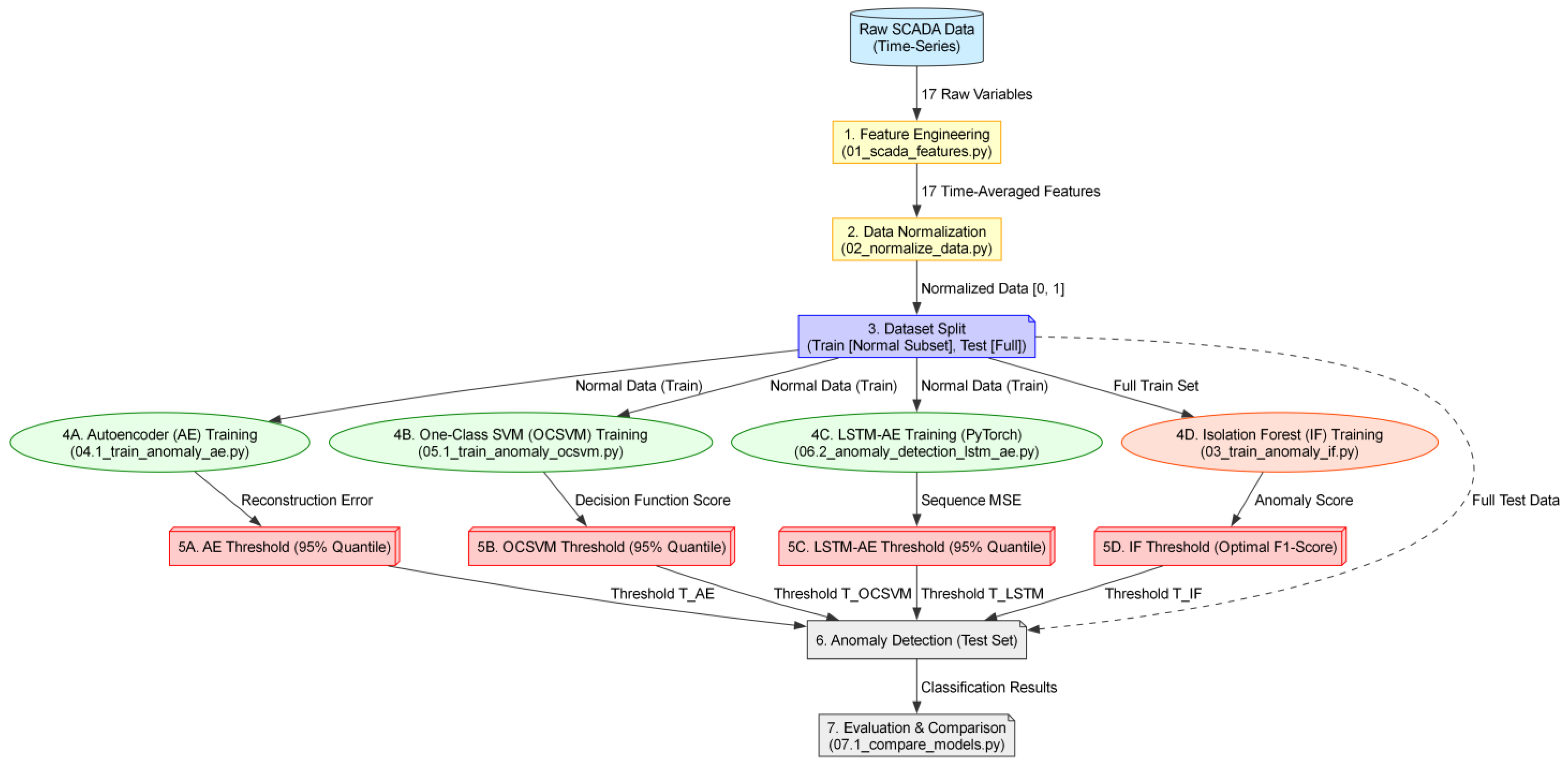
The entire research process, encompassing the stages of data processing, model training, and evaluation, is illustrated in Figure 1.

This process proceeds through the following key phases:

• Preprocessing: Raw data undergoes feature engineering (Listing S1), which involves calculating statistical aggregates (e.g., standard deviation, mean) and time-based difference features from the raw sensor readings. Subsequent Min-Max normalization is applied (Listing S2), followed by splitting into training and testing sets. Crucially, for all models except IF, the training set was filtered to contain only records of the Normal class (0).
• Parallel Training: Four anomaly detection models are trained independently. The Reconstruction-Based and Boundary-Based methods (AE, LSTM-AE, OCSVM) are trained exclusively on Normal data (0), while the Isolation Forest is trained on the full training set (Listing S3).
• Detection and Evaluation: After training, threshold calibration occurs for all four models, followed by the final anomaly detection on the test set, with results evaluated using metrics (AUC, Macro F1-Score, Recall).

3.1. Dataset Characteristics and Class Imbalance

The research was conducted on a publicly available dataset from the SCADA system of an urban wind turbine located in São Paulo, Brazil [7]. The registry contains operational data (electrical, mechanical, environmental) spanning the years 2017–2022. The dataset consists of multivariate time-series records collected with a sampling interval of approximately one minute (1 record per minute). As observed in the raw logs, while the system aims for consistent 60 s steps, minor temporal fluctuations (at the millisecond level) exist due to the SCADA system’s logging latency. The data analyzed is multivariate, comprising 17 processed telemetric features which form the input vector for all models. Detailed descriptions of these features are provided in

Table 3. Final Feature Set Used for Modeling.

Feature Name	Description/Unit
watt_hours	Total generated energy (Wh)
voltage_in	Grid input voltage
voltage_dc_bus	DC bus voltage
voltage_l1, l2	Output voltage of phases L1, L2
current_out	Output current to the grid
power_out	Current output power (W)
power_reg	Regulated power
power_max	Maximum output power
line_frequency	Grid frequency
inverter_frequency	Inverter frequency
line_resistance	Line resistance
rpm	Rotor revolutions per minute
windspeed_ref	Reference wind speed (m/s)
t1, t2, t3	Temperatures (casing, inverter, environment, °C)

.

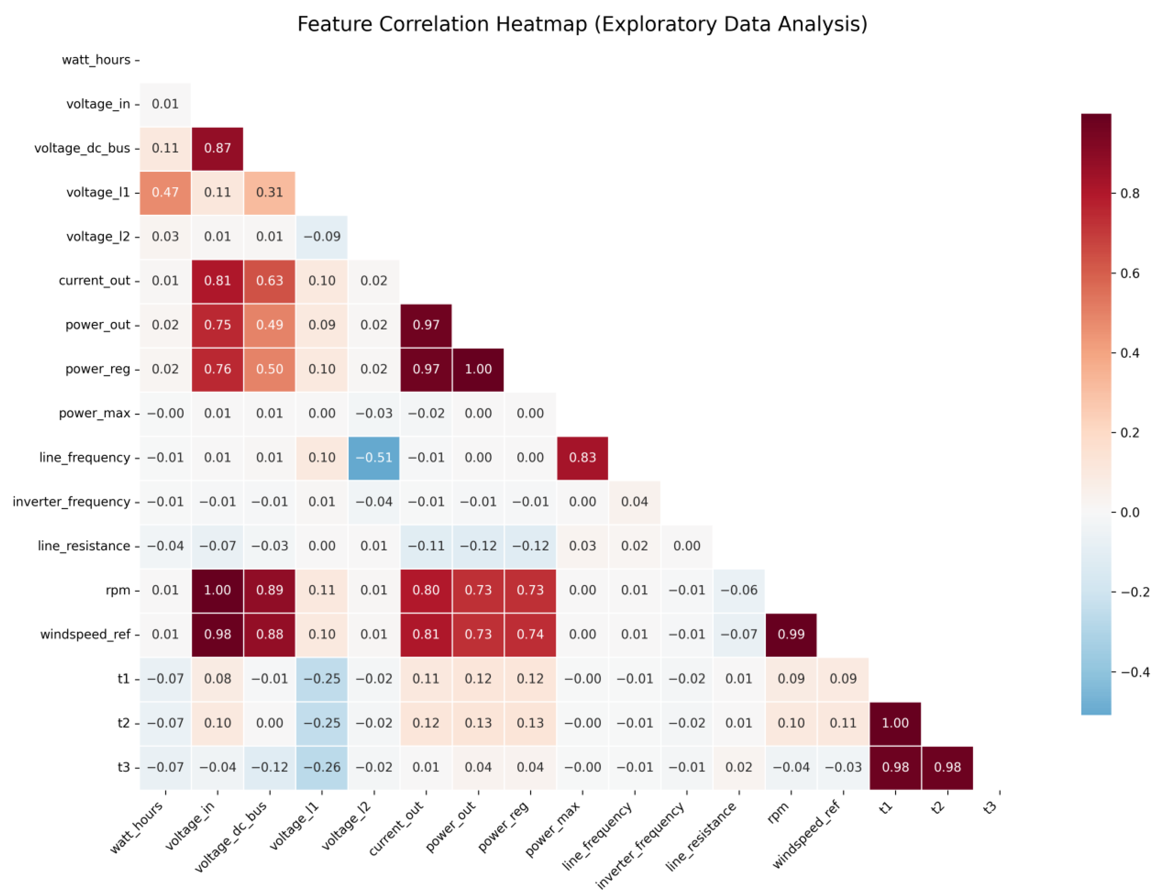
To further understand the interdependencies within the SCADA telemetry, an Exploratory Data Analysis (EDA) was performed. Figure 2 presents the correlation matrix for the 17 selected telemetric features.

The analysis reveals that the ‘Normal’ operational manifold is highly structured, with physical dependencies—such as the near-linear correlation between rotor speed (rpm) and reference wind speed (r ≈ 0.99)—being clearly visible. This high degree of multi-collinearity suggests that the system’s healthy state can be effectively captured in a lower-dimensional latent space.

Classification Definition of Operational States:

• Normal Class (0): Strictly defined as the state “Normal. Run with energy generation” (status code 0), representing the optimal, stable operation of the turbine.
• Anomaly Class (1): Defined as the set of all remaining operational states (including Low Windspeed, Braking, Grid Disconnect, Waiting, High Temp). These states are abnormal from the perspective of maximizing energy production and constitute non-normal operation states, rather than necessarily equipment failure. These sub-states are aggregated into a single Anomaly Class (1) because they all represent a deviation from the optimal operating state (‘Normal. Run’). For the purpose of this binary classification study, we focused solely on the separation between the optimal state and all non-optimal states, rather than sub-classifying specific failure modes.

In the context of industrial Prognostics and Health Management, the definition of a ‘Normal’ state is based on functional optimality rather than statistical frequency. Although the ‘Normal. Run’ state constitutes only 24.27% of the dataset, it is the only state representing the turbine’s design objective—steady-state energy production. All other states (75.73%), despite their higher frequency in this specific urban environment, represent deviations from this objective (e.g., braking, low-wind standby, or technical faults). Therefore, these states are classified as ‘Anomalies’ relative to the optimal operational manifold, justifying the use of anomaly detection algorithms to isolate the desirable production state from all other operational regimes.

While identifying specific failure modes is critical for prescriptive maintenance, this study prioritizes the fundamental task of Anomaly Detection. In SCADA-based monitoring, the primary challenge is often the reliable separation of the optimal operational state (‘Normal’) from all other non-optimal regimes. Establishing a stable ‘Normal’ baseline is a prerequisite for subsequent Fault Diagnosis. By focusing on binary classification under extreme inverted imbalance, we provide a robust foundation for multi-class frameworks that could, in future iterations, differentiate between specific anomaly types such as grid faults, mechanical wear, or sensor drift.

Extreme Imbalance (Inverted Imbalance): A unique feature of this dataset is the inversion of the traditional class imbalance. The total number of records is 1,443,381. As presented in

Table 4. Distribution of records between classes.

Class	Support	Percentage Fraction
Normal (0)	349,791	24.27%
Anomaly (1)	1,093,590	75.73%

, the Anomaly state (1) constitutes the dominant fraction, amounting to 75.73%, while the Normal class (0) is the minority (24.27%).

The Anomaly fraction, at 75.73%, imposes methodological challenges, as the majority of unsupervised algorithms assume that an anomaly is a rarity (an outlier) in the dataset.

3.2. Models Utilized and Thresholding Strategies

The selection of the four algorithms—Autoencoder, LSTM-Autoencoder, One-Class SVM, and Isolation Forest—was driven by the need to compare two fundamental paradigms in unsupervised anomaly detection under the constraint of inverted class imbalance:

• Reconstruction-based vs. Proximity-based methods: AE and LSTM-AE represent reconstruction-based approaches, which learn the internal structure of the “Normal” state. OCSVM and IF represent proximity- and density-based approaches, which define boundaries based on the distribution of data points in the feature space.
• Static vs. Temporal modeling: While AE, OCSVM, and IF process data points as static vectors, the LSTM-AE was included to evaluate whether capturing temporal dependencies and sequences—inherent in SCADA telemetry—provides a significant advantage in identifying anomalies.
• Baseline vs. Deep Learning: OCSVM and IF are widely regarded as industry-standard baselines for anomaly detection due to their efficiency. Comparing them against Deep Learning architectures (AE, LSTM-AE) allows for an assessment of whether the increased computational complexity of neural networks is justified by superior performance in the context of urban wind turbine monitoring.

The following subsections provide a detailed description of these models. For the purpose of comparative analysis, four models were applied, representing Deep Learning Reconstruction-Based methods (AE, LSTM-AE) and Proximity/Isolation-Based methods (OCSVM, IF), all utilizing the 17-feature set, each employing a distinct thresholding strategy.

3.2.1. Autoencoder

Both Autoencoders were trained exclusively on the Normal data (0) to learn the cohesive space of normality.

Autoencoder: The static AE model uses a symmetric architecture with Fully Connected (Dense) Layers. The architecture compresses the 17 input features down to a latent space layer of 8 neurons. The structure is: Encoder: 17 → 16 → 8 neurons; Decoder: 8 → 16 → 17 neurons. ReLU activation was used in the intermediate layers, with Sigmoid on the output layer. This simpler, two-layer architecture was chosen to minimize complexity while effectively capturing the manifold of the normal data.

• Detection Mechanism: Reconstruction Error (MSE).
• Anomaly Threshold: Set to the 95% quantile of the reconstruction error of the Normal data (0). This method offers stability as the threshold is calibrated based on the pure, representative minority class statistics.

LSTM-Autoencoder: This model was introduced to specifically test the influence of temporal dependency modeling. The data was preprocessed into sequences of 90 time steps. The architecture used a stacked LSTM encoder–decoder structure. The encoder consists of two LSTM layers, compressing the input sequence down to a latent space of 16 dimensions (LATENT_DIM = 16). The decoder uses two mirrored LSTM layers to reconstruct the original sequence. The latent vector is repeated across all time steps (90) before decoding.

• Detection Mechanism: Sequence Reconstruction Error (Sequence MSE).
• Anomaly Threshold: Although the initial threshold was set to the 95% quantile of the Normal data’s Sequence MSE (for comparison with AE), the final comparative results were obtained using the Optimal F1-Score Threshold due to the severe instability of the quantile-based approach. (This explains the apparent contradiction in Section 4.)

3.2.2. Proximity/Isolation-Based Methods: OCSVM and IF

These classical ML models rely on separating the data space rather than reproducing it.

One-Class SVM: The OCSVM model was trained exclusively on the training subset of the Normal data (0) using an RBF kernel. This subset represents the 80% train split of the total Normal records (349,791 records). The goal was to find a hyperplane boundary that maximizes the separation of the normal data from the origin in the feature space.

• Detection Mechanism: Decision Function Score (Distance to the separation boundary).
• Anomaly Threshold: Set to the 5% quantile of the Decision Function score of the Normal data. This defines the separation boundary of the learned normality space.

Isolation Forest: The IF model was trained on the entire dataset (Normal + Anomaly).

• Detection Mechanism: Isolation Score (the ease with which a point can be isolated).
• IF Thresholding Challenge (Fraction Matching Method): Due to the inverted imbalance problem, the threshold was manually set to the 75.7% quantile of the anomaly score distribution (Score Samples). This Fraction-Matched Threshold was used as a methodological experiment. Note that the final metrics were obtained using the Optimal F1-Score Threshold. This forced adjustment is hypothesized to cause a complete breakdown of the model’s classification capability in the normal class, despite the model’s fundamental ability to rank anomalies (high AUC).

3.3. Implementation and Analytical Environment

The entire data analysis process, including feature engineering, normalization, the training of all four models (IF, AE, OCSVM, LSTM-AE), and metric evaluation, was automated using Python scripts.

To ensure full reproducibility of the study, all key procedural steps have been made available as Supplementary Materials:

• Feature Engineering (Listing S1)
• Data Normalization (Listing S2)
• IF Training (Listing S3)
• AE Training and Architecture (Listing S4)
• OCSVM Training (Listing S5)
• Time-Series Sequence Preprocessing (Listing S6)
• LSTM-AE Training and Detection (Listing S7)

The experiments were conducted on a workstation equipped with an Intel^® Core™ i5-14400F processor (2.50 GHz), 32 GB RAM, and an NVIDIA GeForce RTX 5060 GPU (8 GB). The models were implemented in Python 3.11.9, utilizing libraries such as Pandas 2.3, Numpy 2.3, Scikit-learn 1.7, Scipy 1.16, TensorFlow 2.20 and Torch 2.10. Key hyperparameters included: Autoencoder–encoding dimension = 8, learning rate = 1 × 10⁻³, batch size = 128; LSTM-Autoencoder–latent dimension = 16, learning rate = 5 × 10⁻⁴, batch size = 512, sequence length = 90 time steps. All models were trained for up to 50 epochs with early stopping to prevent overfitting.

To ensure a robust evaluation under conditions of extreme class imbalance, the Macro F1-Score was adopted as the primary classification metric. Unlike the standard F1-Score or Weighted F1-Score, the ‘Macro’ variant calculates the arithmetic mean of the F1-Scores for each class independently, assigning equal weight to both the minority (Normal) and majority (Anomaly) classes regardless of their support in the test set. This approach is critical for detecting models that fail to identify the minority class, as it prevents the dominant class performance from masking a total collapse of the decision boundary for the ‘Normal’ operation state.

4. Results

This section presents the detailed performance results of all four anomaly detection models—Autoencoder, LSTM-Autoencoder, One-Class SVM, and Isolation Forest—applied to the SCADA dataset under the condition of extreme inverted class imbalance (Anomaly ≈ 75.7%). The analysis is structured to compare the models across two key dimensions: overall discriminative power (AUC) and classification balance (Macro F1-Score) achieved using their respective calibrated thresholds.

4.1. Overall Comparative Performance

The overall performance metrics are summarized in

Table 5. Final comparative performance analysis of all four models using their respective optimized/calibrated thresholds (AE/OCSVM: 95th percentile, IF/LSTM-AE: Optimal F1-Score).

Model	AUC	Macro F1-Score	Recall Normal (0)	Recall Anomaly (1)
Autoencoder	0.9667	0.8962	0.9551	0.9073
LSTM-Autoencoder	0.8987	0.4845	0.0000	1.0000
One-Class SVM	0.9171	0.6703	0.6642	0.8969
Isolation Forest	0.8616	0.4311	0.0000	1.0000

Note: The Isolation Forest metrics reflect its Optimal F1-Score threshold, which yielded the highest classification balance among tested strategies. Even at this optimized threshold, the model resulted in a catastrophic failure for the minority class (Recall Normal = 0.0000), empirically supporting the thesis of threshold instability. The specific methodological experiment involving the Fraction-Matching Method (75.7% quantile) is detailed in Section 4.4.4.

, which consolidates the effectiveness of the distinct methodological approaches (Reconstruction vs. Proximity, Static vs. Temporal) under the unified evaluation framework.

4.2. Discriminative Power (AUC) Analysis

The Area Under the Curve measures the model’s ability to rank anomaly scores correctly, independently of the chosen classification threshold.

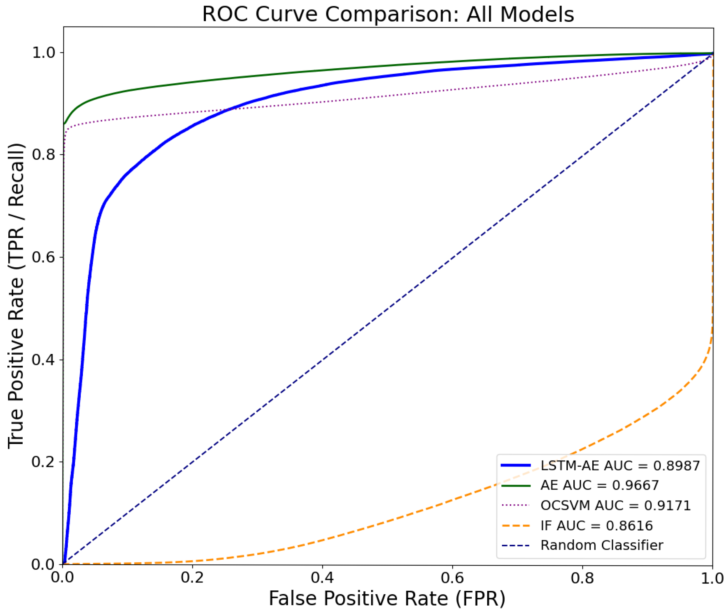
• The Autoencoder demonstrated the highest discriminative power with an AUC of 0.9667. This result positions the static, reconstruction-based approach as the most effective method for separating the two classes across all operating points.
• The One-Class SVM also showed strong performance (AUC 0.9171), followed by the LSTM-Autoencoder with an AUC of 0.8987.
• The Isolation Forest achieved an AUC of 0.8616. While this was the lowest score among the models, this value still indicates a strong ability to rank anomaly scores and is far from representing a failure in the model’s core discriminative power.

The overall comparison of discriminative ability is visually presented in Figure 3.

4.3. Classification Balance and Threshold Stability (Macro F1-Score)

The Macro F1-Score assesses the overall classification effectiveness by averaging the F1-Score for both the Normal (0) and Anomaly (1) classes, providing a robust measure of performance balance under the applied threshold.

• The Autoencoder achieved the highest balance (Macro F1-Score 0.8962). Its key strength was maintaining a high Recall Normal (0.9551), confirming that its threshold, based on the 95% MSE quantile, established a stable decision boundary independent of the statistically dominant anomaly fraction.
• The LSTM-Autoencoder and One-Class SVM exhibited lower classification balance (0.4845 and 0.6703, respectively), primarily due to poor performance in recognizing the Normal class (Recall Normal 0.0000 and 0.6642).
• The Isolation Forest failed completely in binary classification under the necessary threshold constraint, resulting in a Recall Normal of 0.00 and a Macro F1-Score of 0.4311. This empirically validates the hypothesis regarding the instability of fraction-based thresholding for the IF model in the context of inverted class imbalance, despite its strong discriminative performance (AUC 0.8616).

4.4. Detailed Classification Metrics and Threshold Stability

This sub-section provides detailed classification reports for each of the four models, focusing on the resulting Precision, Recall, and F1-Score for both the Normal (0) and Anomaly (1) classes. This analysis confirms the stability of the decision boundary achieved by the distinct thresholding strategies under the inverted class imbalance constraint.

Table 6. Detailed Classification Metrics for the Autoencoder model.

	Class	Precision	Recall	F1-Score	Support
Autoencoder	Normal (0)	0.7681	0.9551	0.8494	349,791
	Anomaly (1)	0.9827	0.9073	0.9440	1,093,590
LSTM-Autoencoder	Normal (0)	0.0000	0.0000	0.0000	69,959
	Anomaly (1)	0.9399	1.0000	0.9690	1,093,501
	Macro Average 1	0.4699	0.5000	0.4845	1,163,460
One-Class SVM	Normal (0)	0.2918	0.6642	0.4054	69,959
	Anomaly (1)	0.9766	0.8969	0.9350	1,093,590
Isolation Forest	Normal (0)	0.0000	0.0000	0.0000	69,959
	Anomaly (1)	0.7570	1.0000	0.8617	1,093,590

Note: ¹ The metrics above reflect the result of the Optimal F1-Score Threshold. The resulting Recall Normal 0.0000 and Recall Anomaly 1.0000 confirm that virtually all test points were classified as anomalies.

provides the full classification reports, confirming the stability of decision boundaries across all models.

4.4.1. Autoencoder: The Best-Balanced Performance

The static Autoencoder, utilizing the 95% MSE Quantile threshold, demonstrated the highest overall classification balance and stability.

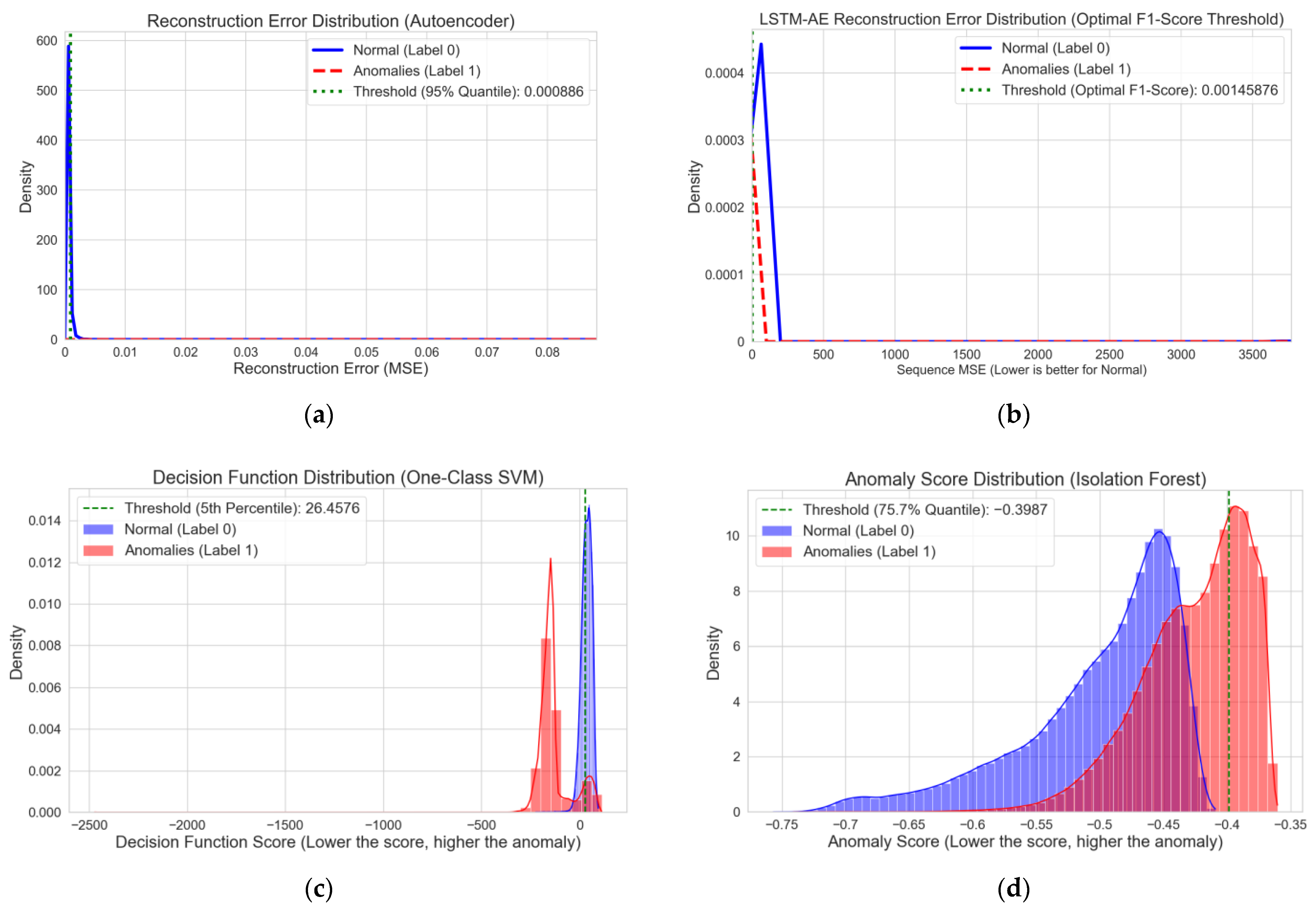
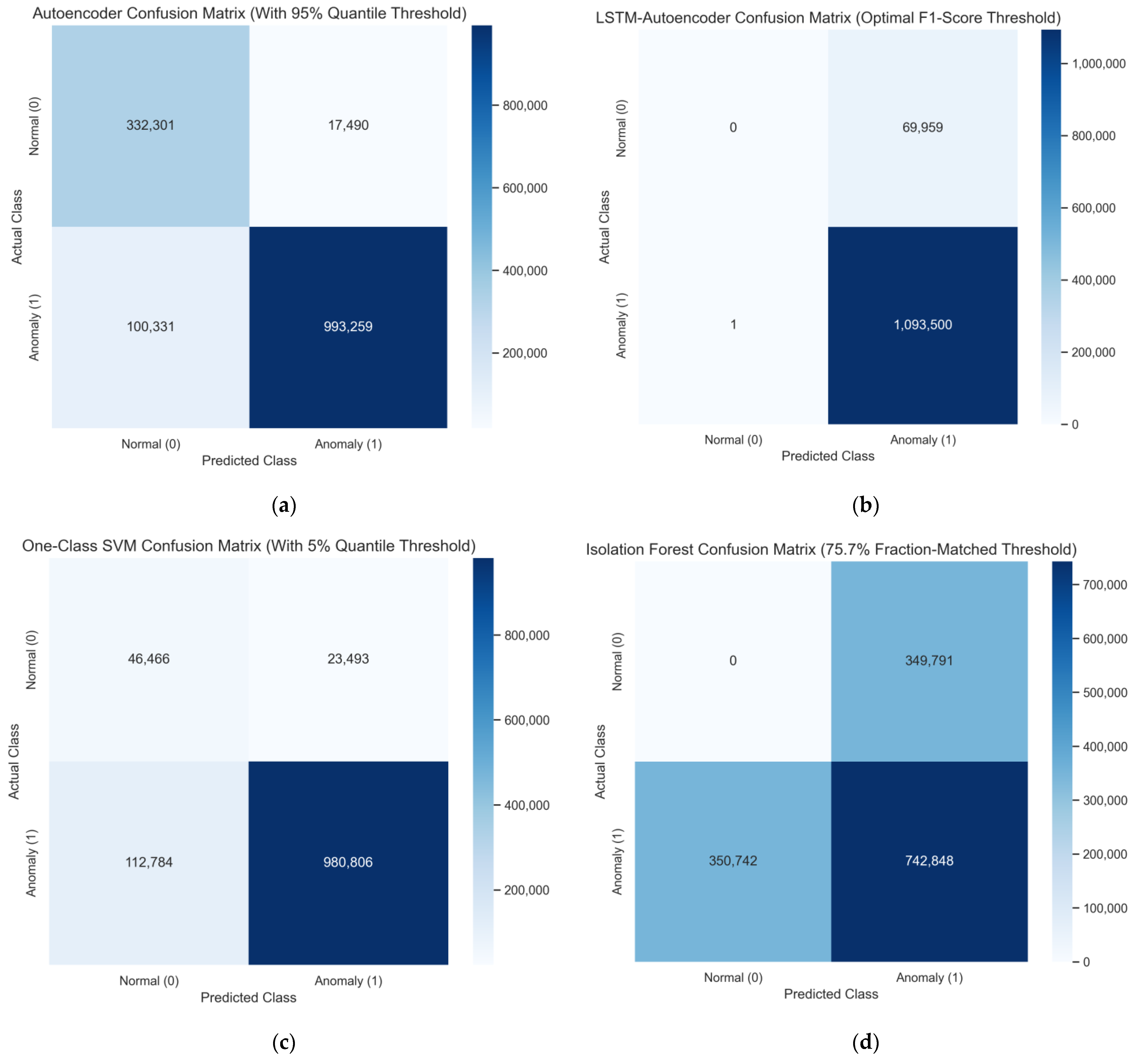
The high Recall Normal (0.9551) confirms that the model successfully minimized False Positives, validating the stability of the reconstruction-error-based threshold. The stability is visually confirmed by the tight distribution of the Normal class error relative to the set threshold (Figure 4a) and the clear classification effectiveness shown in the confusion matrix (Figure 5a).

Although the Autoencoder achieved high Recall for anomalies (0.9073), Figure 4a shows that a portion of anomaly samples exhibits reconstruction errors below the 95% quantile threshold (0.000886), leading to false negatives. This behavior stems from our operational definition of anomalies (non-optimal yet often benign states) and the threshold calibration prioritizing low false-positive rate in SCADA settings. The resulting trade-off yields Recall Anomaly = 0.9073 while maintaining Recall Normal = 0.9551.

4.4.2. LSTM-Autoencoder: Threshold Instability Under F1-Score Optimization

The LSTM-Autoencoder model was introduced to verify the impact of temporal dependency modeling on anomaly detection. While the model demonstrated strong discriminative power, achieving an Area Under the Curve of 0.8987, the resulting binary classification performance suffered from critical threshold instability similar to the Isolation Forest model.

The final classification metrics were obtained using the Optimal F1-Score Threshold (which was 0.00145876), a method applied to maximize the balance between Precision and Recall.

This empirical evidence indicates that the LSTM-AE, despite its ability to model temporal sequences, is highly sensitive to threshold optimization under the severe class imbalance, making it unsuitable for practical deployment in its current configuration.

The distribution of sequence reconstruction errors, though visually distinct (as illustrated in 4b), confirms the narrow margin between Normal and Anomaly scores that forced the F1-optimized threshold to select an extreme operating point. The resulting Recall Normal (0.0000) confirms that the Optimal F1-Score Threshold led to a complete collapse of the decision boundary for the Normal class. Every record was classified as an anomaly, resulting in a catastrophic rate of False Positives (see the results in Figure 5b).

Figure 4b illustrates the collapse induced by the F1-optimized threshold (0.00145876): nearly all samples are classified as anomalies, resulting in Recall Normal = 0.0000 and Recall Anomaly = 1.0000 (Figure 5b). This apparent bias toward anomalies reflects threshold instability under extreme inverted imbalance rather than poor ranking ability (AUC = 0.8987). The overlap of sequence-level error distributions and temporal non-stationarity caused the F1-optimized threshold to select an extreme operating point.

4.4.3. One-Class SVM: Boundary Separation Instability

The One-Class SVM model, utilizing the 5% Decision Function Quantile threshold, demonstrated moderate performance but struggled to maintain classification balance under the inverted imbalance.

The low Precision Normal (0.2918) confirms a high rate of incorrect anomaly predictions. The distribution of the OCSVM Decision Function scores (Figure 4c) shows the resulting overlap near the decision boundary, which is reflected in the confusion matrix (Figure 5c).

4.4.4. Isolation Forest: Instability Under Optimal Thresholding

A comprehensive ablation study was performed on the Isolation Forest model to test its stability under various thresholding strategies, comparing the optimal threshold, the fraction-matched threshold (75.7% quantile), and the standard contamination-based threshold. The results, summarized in

Table 7. Detailed Classification Metrics for the Isolation Forest model.

Threshold Strategy	AUC	Macro F1-Score	Recall Normal (0)	Recall Anomaly (1)
Optimal F1-Score (Highest Balance)	0.8616	0.4311	0.0000	1.0000
Fraction-Matched (75.7% Quantile)	0.8616	0.3398	0.0000	0.6793
Contamination Matched (24.3% Quantile)	0.8616	0.2071	0.4259	0.1371

, confirm that regardless of the calibration method used, the model exhibited fundamental instability in the presence of extreme inverted class imbalance (Anomaly ≈ 75.7%). This led to a Recall Normal of 0.0000 in two of the three scenarios and a severe collapse of the Macro F1-Score (0.2071 to 0.4311).

The Isolation Forest model, even when utilizing the Optimal F1-Score Threshold (which yielded the highest classification balance), failed completely in distinguishing the Normal class. This failure is despite its good discriminative power (AUC 0.8616) and supports the hypothesis of boundary instability under inverted imbalance. The resulting Recall Normal of 0.00 confirms that the optimal decision boundary still collapsed into the core of the Normal distribution.

Note on Methodology: The metrics in Table 5 (Section 4.1) reflect the Optimal F1-Score threshold. A separate methodological experiment using the Fraction-Matched Threshold (75.7% quantile, threshold −0.3987) was conducted to demonstrate threshold instability, as illustrated in the scoring distributions and confusion matrices (Figure 4d and Figure 5d).

Figure 4d and Figure 5d confirm that fraction-matched thresholding (75.7% quantile, −0.3987) collapses the decision boundary, labeling nearly all samples as anomalies and yielding Recall(Normal) ≈ 0. This failure mode persists even under alternative calibration strategies (Table 7), evidencing fundamental threshold instability for IF in the inverted imbalance scenario.

4.5. Qualitative Interpretation of Model Performance

The divergent performance of the models can be attributed to their fundamental learning paradigms. The Autoencoder outperformed other models because its reconstruction-based objective specifically learns the compact manifold of “Normal” operation. Under inverted imbalance, where anomalies are the majority, the AE’s strategy of ignoring the anomaly distribution during training provides a stable baseline.

In contrast, the Isolation Forest and LSTM-AE suffered from threshold collapse. For the IF, the inherent mechanism of isolating points via random partitioning becomes mathematically unstable when the “outliers” (Normal class) are statistically indistinguishable from the dense clusters of anomalies in the feature space. While the LSTM-AE successfully captured temporal patterns (high AUC), the high variance in its sequence reconstruction errors—caused by the complex, non-linear nature of SCADA transitions—prevented the formation of a sharp decision boundary.

To further validate these qualitative observations with statistical rigor, DeLong’s test was applied to evaluate the significance of the differences in discriminative power between the models.

4.6. Statistical Significance of AUC (DeLong’s Test)

DeLong’s test was conducted to determine the statistical significance of the difference between the AUC of the Autoencoder model (Reference) and the other models. A p-value below 0.05 indicates a statistically significant difference in discriminative power.

The results of DeLong’s test, summarized in

Table 8. Statistical Significance of AUC Comparison (DeLong’s Test).

Comparison (AE: 0.9667)	AUC (Compared Model)	Z-Statistic	p-Value	Significant (p < 0.05)
AE vs. LSTM-AE	0.8987	−537.8159	0.000000	Yes
AE vs. OCSVM	0.9171	−496.2755	0.000000	Yes
AE vs. IF	0.8616	−2463.6534	0.000000	Yes

, empirically confirm the superiority of the Autoencoder model. The p-values for all comparisons are p < 0.000001, indicating a highly statistically significant difference between the AE’s AUC (0.9667) and the performance of the LSTM-AE, OCSVM, and IF models. This validates the conclusion that the static, reconstruction-based approach is the most effective model for ranking anomalies in the context of extreme inverted class imbalance.

4.7. Computational Efficiency and Real-Time Suitability

A critical factor for SCADA systems is the computational cost of the model. The total inference time required to process the entire test dataset (approximately 1.44 million records) was measured for each model. The results confirm a significant trade-off between model complexity and processing speed (

Table 9. Inference Time Comparison (Total Test Set).

Model	Inference Time (ms)	Inference Time (Seconds)
One-Class SVM	143,874.45	143.87
LSTM-Autoencoder	18,027.87	18.03
Autoencoder	10,420.93	10.42
Isolation Forest	3940.07	3.94

).

While the Isolation Forest demonstrated the highest computational efficiency (Table 9), its diagnostic utility was severely limited by the thresholding challenges discussed in Section 4.4.4. Conversely, the One-Class SVM, while providing robust ranking, exhibited an inference time nearly 14 times longer than the Autoencoder, which may limit its application in high-frequency real-time SCADA environments.

To provide a holistic overview of the experimental findings,

Table 10. Comparative Summary of Algorithm Characteristics and Performance under Inverted Imbalance.

Algorithm	Learning Paradigm	Key Strength in This Study	Primary Weakness/Failure Mode
Autoencoder	Reconstruction	High boundary stability; effectively ignores majority anomaly noise.	Requires careful latent space tuning to avoid over-compression.
OCSVM	Boundary-based	Robust ranking; clear distance-to-boundary metric.	High computational cost (inference time) and sensitivity to kernel parameters.
LSTM-AE	Temporal Reconstruction	Excellent at capturing sequential dependencies and trends.	Severe threshold instability; reconstruction error variance is too high for binary split.
Isolation Forest	Partition-based	Exceptionally fast; good at ranking anomaly severity.	Catastrophic failure in binary classification; threshold collapses into the Normal distribution core.

synthesizes the strengths and weaknesses of each algorithm. This qualitative summary highlights the trade-offs between learning paradigms, stability under inverted imbalance, and operational efficiency, serving as a guide for selecting the optimal model for urban wind turbine monitoring.

5. Discussion and Conclusions

This chapter provides a detailed interpretation and discussion of the obtained comparative results, with a particular focus on the fundamental difference in threshold stability between reconstruction-based and proximity-based methods under the unique challenge of inverted class imbalance. Based on empirical evidence from all four models (AE, LSTM-AE, OCSVM, IF), final conclusions are formulated, key engineering implications for SCADA systems are defined, and limitations and future research directions (Future Works) are outlined.

5.1. Final Conclusions and Methodological Verification

The comparative analysis clearly demonstrated (Table 5) that the static Autoencoder model is methodologically and empirically superior for the problem of binary anomaly classification where the “normal” state constitutes the minority.

5.1.1. Superiority of Reconstruction-Based Thresholding (AE vs. IF/OCSVM)

The main conclusion of this research pertains to the critical impact of the thresholding strategy in the scenario of inverted class imbalance.

• AE’s Success (Stable Boundary): The AE model, trained exclusively on the rare normal class, learned a tight, low-dimensional representation (manifold). The resulting classification threshold, based on the internal statistics of the pure Normal class (95% MSE Quantile), proved to be robust and independent of the 75.7% anomaly fraction. This led to balanced effectiveness (Macro F1-Score 0.8962) and minimal False Positives (Recall Normal 0.9551).
• IF’s Failure (Threshold Instability): The Isolation Forest model demonstrated an inherent instability under the inverted class imbalance, resulting in a Recall Normal of 0.00 across two distinct thresholding scenarios. This catastrophic failure was observed even when using the dynamically determined Optimal F1-Score threshold (Table 5, Macro F1-Score = 0.4311), proving the algorithm’s decision boundary is fundamentally inadequate for this classification task. Furthermore, the use of the Fraction-Matched Threshold (Section 4.4.4) was an intentional methodological experiment. This experiment was designed to empirically test the assumption that a proximity-based algorithm’s score distribution could be reliably coupled with the externally observed class fraction (75.7%). The result of this test, showing the model’s complete collapse (Table 6), strongly supports the thesis that IF cannot be used as a robust binary classifier in the inverted imbalance setting, regardless of the calibration strategy employed.
• OCSVM Instability: The One-Class SVM, although achieving a strong AUC (0.9171), exhibited poor stability in classification balance (Macro F1-Score 0.6703). Its low Precision Normal confirms that the rigid boundary separation method, even when trained only on the normal class, struggled to minimize False Positives under the pressure of the dominant anomaly distribution.

5.1.2. Impact of Temporal Modeling (AE vs. LSTM-AE)

The analysis of the LSTM-Autoencoder provides critical insight into the nature of anomalies in this specific SCADA dataset.

• High Anomaly Recall (1.0000): The LSTM-AE achieved the highest Recall Anomaly of all models, indicating that sequential modeling can effectively capture anomalies defined by a breakdown in time-series patterns.
• Lower Overall Performance: Despite high Recall Anomaly, the model’s lower AUC (0.8987) relative to the static AE (0.9667) and poor Recall Normal (0.0000) suggest that the temporal dependencies within the sub-optimal operational states (the 75.7% anomaly class) are often simple or non-critical, or that the static feature set already captured most of the necessary information. The high rate of False Positives suggests that the sequential error distribution overlapped significantly with the normal state, making the threshold unstable.
• Conclusion: For this specific dataset, the added complexity of temporal modeling (LSTM-AE) did not justify the performance gain compared to the robust, static AE.

5.2. Engineering Implications for SCADA Systems

In the context of deployment within industrial SCADA monitoring systems, the findings offer clear guidelines:

• Prioritize Reconstruction: The Autoencoder model is strongly recommended for deployment in environments characterized by inverted imbalance, due to its superior reliability and the stability of its decision boundary.
• Reliability of Normal State Identification: High Recall Normal (≈95%) minimizes False Positives, which is essential for maintaining operator trust and reducing alarm fatigue in critical infrastructure.
• Threshold Stability: The AE thresholding method, based on the internal statistics of the pure normal subset, ensures that the model will maintain its performance regardless of dynamically changing anomaly fractions in the live data stream.
• Avoid Fraction-Based Thresholding: Proximity methods like IF, when constrained by fraction-based thresholds, are unsuitable for classification under inverted imbalance.

5.3. Limitations

This analysis has the following limitations, which must be considered when interpreting the results:

• Data Scope: The research is based on data from a single urban wind turbine. The results may not be fully generalizable to large-scale wind farms or different operational environments.
• Anomaly Definition: The definition of anomaly is broad (it encompasses all suboptimal states). Deployment in a production environment would require further threshold calibration to distinguish critical equipment failures from routine operational states (e.g., Low Windspeed).
• Temporal Complexity: The LSTM-AE results suggest that more complex anomaly patterns might require advanced temporal models (e.g., Transformers, as noted in Section 5.4.1), or that the current feature set is insufficient to capture subtle temporal dependencies in the SCADA data.

5.4. Future Research Directions

Based on the experimental findings—specifically the methodological stability of the static Autoencoder and the identified threshold instability in temporal and proximity-based models under inverted imbalance—the following future research directions are recommended.

5.4.1. Advanced Temporal and Attention-Based Modeling

Although the LSTM-AE demonstrated high discriminative power (AUC 0.8987), it suffered from critical threshold instability, leading to a collapse of the “Normal” class boundary. This suggests that standard sequential modeling requires enhancement to produce more distinct anomaly scoring margins. Future work should explore:

• Transformer Networks: Utilizing architectures based on attention mechanisms, such as Informer and TimesNet, which are specifically designed to capture complex multivariate relationships and long-term sequential dynamics in SCADA time series [21].
• Temporal Feature Optimization: Refining the feature set and sequence lengths to better isolate temporal anomalies that remained indistinguishable from the majority anomaly fraction in the current static-oriented framework.

5.4.2. Transfer Learning and Fleet-Wide Robustness

A primary limitation of this study is its focus on data from a single urban wind turbine. The extreme inverted imbalance (75.7% anomalies) identified here necessitates validation on a broader fleet scale. Unsupervised Transfer Learning represents a crucial strategy to address this, allowing knowledge acquired from a large, diversified fleet (source domain) to be leveraged for new turbines (target domain) [22]. Such techniques can mitigate domain shift and potentially address data imbalance through pre-training on large bases of normal operations [22]. However, since training on multiple turbines does not always guarantee improved performance, further investigation into fine-tuning decoders and adaptive threshold modification is required [23].

5.4.3. Hybrid Architectures and Ensemble Models

The results in Section 4.4.4 indicated that while Isolation Forest retains strong ranking capabilities (AUC 0.8616), its decision boundary in the original feature space is unstable. To optimize performance, future research should investigate:

• Hybrid Latent-Space Models: Using an Autoencoder for dimensionality reduction and normal state feature extraction, followed by applying algorithms like IF or OCSVM in the reduced-dimensional latent space [24]. Such synergy can potentially combine the AE’s ability to model the normal manifold with the speed or specific discriminative properties of ML.
• Ensemble Deep Learning: Implementing ensemble networks to combine predictions from multiple model variants, thereby reducing uncertainty and minimizing false alarms [25].

5.4.4. Intelligent Diagnostic Reporting (RAG)

To extend the decision-making process beyond raw binary classification, integrating PHM diagnostic outputs with Retrieval-Augmented Generation (RAG) systems represents a vital direction. This requires a refined methodology for selecting Large Language Models (LLMs) and tuning vector databases to ensure that generated reports are accurate, context-aware, and computationally efficient [26].