Article

Predicting Demand in Supply Chain Management: A Decision Support System Using Graph Convolutional Networks

by
Stefani Sifuentes-Domínguez
1,
Jose-Manuel Mejia-Muñoz
1,
Oliverio Cruz-Mejia
2,*,
Rubén Pizarro-Gurrola
3,
Aracelí-Soledad Domínguez-Flores
3 and
Leticia Ortega-Máynez
1
1
Departamento de Ingeniería Eléctrica, Instituto de Ingeniería y Tecnología, Universidad Autónoma de Ciudad Juárez, Ciudad Juarez 32310, Mexico
2
Departamento de Ingeniería Industrial, FES Aragón, Universidad Nacional Autónoma de México, Nezahualcóyotl 57171, Mexico
3
Departamento de Sistemas y Computación, Tecnológico Nacional de México, Instituto Tecnológico de Durango, Durango 34080, Mexico
*
Author to whom correspondence should be addressed.
Future Internet 2026, 18(1), 26; https://doi.org/10.3390/fi18010026
Submission received: 27 November 2025 / Revised: 30 December 2025 / Accepted: 31 December 2025 / Published: 2 January 2026
(This article belongs to the Special Issue Machine Learning and Internet of Things in Industry 4.0)

Abstract

This work addresses the problem of demand forecasting in supply chain management, where the consolidation of scattered and heterogeneous data and the lack of precise forecasting methods generate operational inefficiencies, resulting in increased backorders and high inventory costs. To tackle these challenges, we propose a novel Decision Support System that jointly integrates an intelligent processing engine based on Graph Neural Networks (GNNs) for time series forecasting. Our approach lies in explicitly modeling the demand prediction task as a Multivariate Time Series forecasting problem on a causal dependency graph. Specifically, we use a GCN to process a graph where the nodes represent the target demand and key exogenous variables (Consumer Sentiment Index, Consumer Price Index, Personal Income, and Unemployment Rate), and the edges explicitly encode the interdependencies and causal relationships among these economic factors and demand. Unlike previous applications of GNNs in supply chain management, which typically focus on inventory networks or single-factor interactions, our approach uses GCN to dynamically capture the temporal interactions among multiple macroeconomic and internal series on future demand. We compare our method with other machine learning algorithms for demand forecasting. In the experiments conducted, the proposed GCN approach can accurately predict the abrupt changes that appear in demand behavior over time, whereas the other comparison methods tend to excessively smooth these transitions.

1. Introduction

Within the domains of industrial engineering, manufacturing, and production systems, demand forecasting is fundamentally challenged by the integration of highly dispersed, heterogeneous, and large-scale data sources. According to [1], the variety of data sources which include historical sales, market trends, economic conditions, and seasonal variables complicates the process of interpretation and analysis. In addition, the large volume of available data can hinder the identification of patterns and trends relevant for decision making.
The problem of demand forecasting in supply chain management is mainly manifested as a lack of accuracy in the information and the use of inadequate forecasting methods, which generates critical operational inefficiencies that directly affect customer service and inventory costs. Inaccurate forecasts, however, can generate significant difficulties, such as an increase in backorders and storage costs, due to demand being estimated below or above the actual value [2].
Such inaccuracies result in operational inefficiencies, dissatisfied customers, and significant financial losses, underscoring the need for robust forecasting methodologies [3]. Specifically, the challenge of forecasting customers’ future demand has consistently plagued supply chain systems, impacting decisions ranging from optimal inventory levels at distribution centers to the required production volumes at manufacturing plants [4].
To be able to manage the supply chain, it is important to accurately forecast demand. This is because it has an impact on key decisions related to planning, inventory control, and the optimal allocation of resources [5]. The ability to accurately predict future demand not only helps minimize the costs associated with excess or shortage of inventory, but also enables organizations to quickly adapt to market changes [6]. In this context, it is important to highlight that the deployment of appropriate tools, such as Decision Support Systems (DSSs), can significantly enhance data interpretation, thereby enabling more informed and efficient decision processes.
Evidence demonstrates valid solutions and significant effects. According to [7], 67% of companies deal with lack or excess of inventory every day. Excessive inventories make the supply chain vulnerable and generate expenses due to obsolescence [8]. Nevertheless, accuracy in forecasting produces advantages that can be measured. According to [9], Walmart was able to reduce inventories by 20% and increase forecast accuracy by 15%; for its part, Procter & Gamble achieved a 30% reduction in inventories and a 20% increase in accuracy thanks to artificial intelligence algorithms. Accurate forecasting makes it possible to anticipate market demands, properly regulate inventory levels, and prevent stockouts or overstocking [10].
In this work, we propose a DSS with a demand prediction module. Due to the growing flow of data coming from both the external economic environment and internal business processes, the creation of an automated tool to prescribe scenarios that account for external factors from this complex environment has become imperative. The complexity of modern strategic management has increased, as it must address problems such as uncertainty generated by rapid and unexpected changes, as well as the difficulty of selecting and analyzing the interconnections among factors.
The proposed DSS, is conceived as an intelligent human–computer interface, incorporates the influence of exogenous variables that indirectly impact the production system. In this work, the demand prediction task is formulated as a multivariate time-series forecasting problem defined over a causal dependency graph, where relationships among situational and macroeconomic factors are explicitly modeled. The causal relationships among these factors are identified using a machine learning–based approach, specifically AdaBoost, enabling the construction of an interpretable and data-driven dependency graph. For demand prediction, we employ graph neural networks (GNNs) as a suitable approach to improve demand forecast accuracy, as they dynamically capture the interactions between demand and multiple exogenous variables through the underlying graph structure.
By integrating the resulting GNN-based demand forecasts directly into the decision-support logic, the proposed framework tightly couples prediction and optimization within a unified DSS, thereby enhancing both theoretical modeling of complex demand drivers and practical decision-making in real-world production and inventory planning contexts.

2. Literature Review

The DSS is a computerized tool designed to assist in solving complex problems. According to [11], first introduced by Gorry and Scott-Morton in 1971, the DSS has evolved significantly in structure and technology. It stands out for its ability to address customized and unique problems, with a significant presence in the manufacturing sector, particularly in areas such as the supply chain of medicines, fertilizers, etc. In addition, the DSS is a key tool across various industries, from agriculture to e-commerce, optimizing their supply chains.
The transformation from DSS to Intelligent Decision Support System (IDSS) was driven by the incorporation of AI. The evolution from basic data analyses in the 1980s to systems with components such as neural networks, fuzzy logic, intelligent agents, and hybrid architectures provide real-time support and predictive analytics. The current state of the art in the integration of AI and ML into IDSS for demand forecasting shows significant progress. As information filtering methods that aid in decision-making, recommender systems have continued to evolve. However, collaborative and content-based strategies are not always the most suitable for every situation [12].
Specifically, in production planning, the DSS offers a structured approach for analyzing data, modeling scenarios, and evaluating options, contributing to operational efficiency by providing information for decision-making [6]. In the automotive industry, [13] present a DSS specifically for demand planning. This system, based on supervisory control theory, includes demand monitoring and forecasting, tools tailored to the automotive sector, and automated processes. The DSS enables companies to optimize operations and make proactive decisions in a changing market. The proposed scenario method guides companies in identifying key variables, creating market scenarios, evaluating risks, and strategic planning. This iterative and adaptable approach improves decision-making and market adaptability.
Similarly, [14] developed an intelligent DSS for production and control planning of the assembly of complex products, based on a weighted sum model and an artificial neural network. This tool uses intelligent algorithms that automatically adjust parameters such as weights and learning rates, improving design efficiency and accuracy in predictions. The weighted sum model algorithm facilitates informed decisions by adapting to market changes, optimizing management for products.
In the automotive industry, [15] introduce a DSS called GUEST, which combines human decision-making with fast algorithms to guide strategic production allocation decisions. This DSS not only optimizes production but also incorporates sustainability criteria, strengthening the sector’s resilience. It is used by manufacturing engineering managers for scenario analysis and decision-making, demonstrating its applicability and effectiveness. The results highlight the relevance of a well-structured DSS for understanding business networks and creating value.
Global literature highlights cutting-edge models for making predictions supported by ML, such as decision trees, deep neural networks, and ensembles, which have demonstrated their ability to increase accuracy in demand estimation. Significant research includes the use of hybrid models and adaptive approaches that take into account trends, seasonal patterns, and exogenous events to produce more robust forecasts [16].
The IDSS that use neural networks, ensemble models, and support vector regression significantly improve the accuracy of demand forecasts in the supply chain. By doing so, they achieve error reductions between 3 and 4 times lower than traditional methods, reaching the most precise calculation in 95% of cases [17].
IDSS that use methods such as neural networks (including LSTM and their improved versions), support vector regression, and hybrid or ensemble models achieve significant advancements in demand forecasting in the supply chain [18]. Compared to conventional approaches, such as exponential smoothing, moving averages, and Autoregressive Integrated Moving Average (ARIMA), these systems show much lower forecasting errors in the pharmaceutical, automotive, energy, manufacturing, and retail sectors [17].
On the other hand, GNNs are used in supply chain demand prediction through innovative methodological approaches that capture complex spatial and temporal dependencies. GNNs enhance forecasting accuracy by allowing methodologies to uncover latent dependencies and address temporal complexities, outperforming, in some cases, traditional models like MLPs and LSTMs in single-node demand forecasting tasks [19]. The use of GNNs to treat companies as nodes and their relationships as edges, aggregating node and edge information to improve demand forecasting accuracy in supply chain management, outperforming traditional algorithms [20].
GNNs were employed for example in [21] were it is developed CIGNN, which dynamically incorporates evolving contextual information into demand forecasting, addressing limitations of fixed-context traditional models. In [22] it is proposed efficient architectures that reduce computational complexity, enabling GNNs to handle large, complex networks. These innovations collectively enhance forecasting accuracy by leveraging graph-based representations of intricate supply chain interactions.
Macroeconomic indicators are increasingly recognized as critical exogenous factors for enhancing demand forecasting and supply chain decision-making. The work in [23] found that predictive analytics incorporating external factors like macroeconomic variables can improve demand planning, while in [3] it is emphasized that traditional statistical models often fall short by neglecting complex variables, highlighting the importance of integrating diverse economic indicators.
Macroeconomic indicators significantly enhance demand forecasting accuracy and supply chain decision-making by providing external economic context beyond traditional sales data. Multiple studies demonstrate the value of incorporating these indicators. For example, in [24] it is found that including macroeconomic variables like Consumer Price Index and Consumer Sentiment Index in predictive models provides greater explanatory power, outperforming models without such external information. In another work, in [25] it is achieved a 54.5% reduction in forecasting error by using leading macroeconomic indicators, while [26] reported 18.8% accuracy gains over existing forecasting processes.
Despite these advances, existing studies still present several limitations when applied to dynamic and data-heterogeneous supply chain environments. The most significant gaps identified in the past five years are the limited generalization of models across various contexts, the insufficient analysis of qualitative and external factors (such as policies and market trends), and the lack of assessment regarding how the level of collaboration between humans and AI systems is affected. Likewise, there is a major opportunity to improve the adaptability of predictions by incorporating real-time data and developing explainable models [16].

3. Materials and Methods

3.1. Current Demand Forecasting Methods

Demand forecasting in supply chain management has traditionally relied on a range of quantitative and data-driven methods with specific advantages and limitations. Classical statistical approaches, such as moving averages, exponential smoothing, and ARIMA models, are widely used due to their interpretability and low computational cost. However, these methods assume linear relationships and stationarity, which limits their ability to capture complex patterns, nonlinear dynamics, and abrupt demand changes [17].
Machine learning techniques, including linear regression, decision trees, Random Forest, Gradient Boosting, and AdaBoost, have gained popularity for demand forecasting due to their flexibility and improved predictive performance. Tree-based and ensemble methods can model nonlinear relationships and interactions among variables, offering better accuracy than linear models. Nevertheless, these methods often treat input variables independently and do not explicitly model structured relationships among multiple time series or external factors, which may reduce their effectiveness in highly interconnected environments [16].
More recently, deep learning models such as recurrent neural networks (RNNs), LSTM networks, and temporal convolutional networks (TCNs) have been applied to demand forecasting, demonstrating improved performance in capturing temporal dependencies. Despite these advances, most deep learning approaches still rely on vector-based representations and struggle to explicitly encode relational dependencies among demand and exogenous variables [27].
These limitations motivate the exploration of graph-based learning approaches. GNNs provide a natural framework to represent demand and external factors as interconnected nodes, allowing the model to learn both temporal patterns and relational dependencies. This capability directly addresses the shortcomings of traditional statistical, machine learning, and deep learning models, and forms the methodological basis for the proposed DSS presented in the following sections.

3.2. The Decision-Making Process

In business, decision-making is essential for solving problems and situations. It is a frequent activity that involves all organizational levels, from assistants to chief executives. The impact of these decisions on the organization depends on the managerial level at which they are made. Decision-making involves obtaining and evaluating information, identifying alternatives, selecting the best solution, and applying it. Managers lead this process, establishing the rules or methods to follow [28]. This generic process is later instantiated and adapted specifically to demand forecasting in Section 4, where each stage is operationalized using data-driven forecasting and exogenous factors.
Stages of Decision-Making.
  • Determination of the need for a decision: Identify and define a situation that requires action, understanding its causes.
  • Identification of the criteria: Detail the problem, analyze and validate solutions.
  • Assigning weight to each criterion: Evaluate alternatives considering relevant factors and the importance of each criterion.
  • Development of possible alternatives: Search for and assess solutions that represent specific values for the decision variables.
  • Evaluation of solution alternatives: Integrate data, information, and experience to evaluate options, acknowledging the presence of uncertainty.
  • Selection of the optimal solution: Consider quality, risk, and context to choose the best solution.
Although the process mentioned above is important in fundamental decision-making, the introduction of information systems, such as a DSS, has innovated this practice. When implementing a DSS to improve this process, it is essential to take into account several relevant aspects [28]:
  • Maintain an efficient flow of information to achieve optimal business results.
  • Promote effective communication to keep everyone informed about decisions and changes.
  • Implement the appropriate technical infrastructure to ensure the proper functioning of the DSS.
  • Consider organizational culture to address resistance to change and ensure system adoption.
  • Establish adequate planning and a clear organizational strategy to support the integration of information within the company.

Typology of Decisions

To understand how a DSS supports decision-making, it is essential to explicitly define the typology of decisions considered in this work. In this study, decisions are classified into structured, semi-structured, and unstructured categories. Structured decisions, also called programmed decisions, are repetitive and have clear solutions, such as replenishing inventory. To optimize them, rules are established under normal conditions, and exceptions are escalated to higher levels. Unstructured decisions, such as deciding whether to enter or exit a market, lack fixed criteria and rely on personal preferences, making them the most uncertain and managerial-level decisions. Semi-structured decisions, such as developing a marketing plan, combine defined criteria with human judgment [28].
This typology provides the conceptual basis for the DSS, clarifying which decisions can be automated, which require managerial judgment, and how the system supports different decision levels within the demand forecasting context. This typology is later mapped onto the DSS architecture presented in Figure 1, where structured decisions are primarily supported by automated data processing and modeling modules, while semi-structured decisions involve user interaction and scenario analysis, and unstructured decisions rely on managerial interpretation of the DSS outputs.

3.3. Decision Support System

In a DSS, it is important to understand the activities: input, storage, processing, and output of information, which may include automated interfaces. The configuration and functions of a DSS vary depending on the context and specific needs [29]. Figure 1 proposes a methodological design for the conceptual architecture of the system, composed of five main modules: database, data processing, modeling and simulation engine, user interface, and results evaluation. These elements are articulated in an iterative flow that allows continuous feedback between data input, analytical processing, and result interpretation.
The architectural components of the DSS, illustrated in Figure 1, are described below.
User Interface. The user interface facilitates user–system interaction with forms, graphics, and controls. It includes data entry forms, interactive charts, adjustable controls, dropdown menus, alerts, and user guidance.
Data Acquisition and Preprocessing. This component provides tools for extracting and preparing data for analysis. It involves data connectors, cleaning, normalization, integration, transformation, and data validation.
Database. The database stores crucial data for decision-making, both historical and real-time. It contains relevant data, parameters, metadata, management tools, and query functions.
Processing Engine. The processing engine performs complex analyses using algorithms and data mining tools. It includes predictive algorithms, optimization models, data mining, simulation, inference rules, and logic.
Modeling and Simulation. This module allows the creation of models to understand decisions. It offers functions to build models, define variables, simulate, validate, and visualize results.
Visualization Tools. Visualization tools present data intuitively using charts, dashboards, and maps. They include various types of charts, interactive dashboards, maps, filtering and zoom functions.
Results Evaluation. This component analyzes the validity and robustness of the results. It includes metrics, sensitivity analysis, hypothesis testing, risk assessment, and report generation.
Collaboration and Communication. This module facilitates collaboration and communication among users. It involves data sharing, comments, notifications, export and import of information, and data security.

3.3.1. Data Required for Measurement and Analysis

The data available for measuring and analyzing demand include historical sales, customer behavior. market trends, economic factors and seasonal variables.

3.3.2. Measures to Monitor Success

The measures that can be monitored to indicate success in demand forecasting include forecast accuracy, optimized inventory level, reduction in costs associated with inventory management and customer satisfaction.

4. Development of the Decision Support System

Supply chain management is a main area for improving efficiency and competitiveness of companies. DSSs can play an important role in them by providing tools and techniques for informed decision-making. Therefore, implementing a DSS in demand forecasting is important to improve the accuracy and reliability of future projections in Industry 4.0 [11].
The improvement in forecasting will be achieved because decision-makers will be able to analyze complex data, model scenarios, and evaluate alternatives efficiently through a DSS, with the intention of facilitating informed, evidence-based decision-making to optimize production planning and management [29].

4.1. Methodology for Decision-Making in Demand Forecasting

The following section describes the methodology adopted for decision-making in the context of demand forecasting. This methodology represents an adaptation of a generic decision-making framework to the specific requirements of demand prediction within a DSS. The proposed approach structures the forecasting process into a sequence of interrelated stages that guide the identification of relevant variables, the evaluation of external influences, and the interpretation of results to support informed managerial decisions.
The methodology emphasizes the integration of analytical reasoning, data-driven modeling, and scenario analysis to support strategic and operational decision-making. By structuring the forecasting process into well-defined stages, the approach facilitates transparency, traceability, and adaptability in the analysis of demand dynamics.
Methodology for Decision-Making in demand forecasting:
  • Identifying the need for forecasting. The process begins by recognizing the strategic importance of anticipating demand fluctuations. This step ensures that forecasting efforts are aligned with organizational goals and decision-making needs.
  • Definition of forecasting criteria establish clear criteria for forecasting, including relevant time horizons, granularity, and performance metrics. These criteria guide the selection of models and evaluation frameworks.
  • Definition of exogenous factors affecting demand. Identify external variables such as macroeconomic indicators, seasonality, competitive actions, and policy changes that influence demand. These factors form the basis for scenario construction.
  • Evaluation of the impact of each factor. Assess the relative influence of each exogenous variable on demand through statistical analysis or expert weighting. This enables the development of scenario-based models that reflect diverse market conditions.
  • Evaluation of results analyze forecasting outputs across scenarios to quantify sensitivities, validate model performance, and identify potential risks. This step supports strategic planning and risk mitigation.
  • Monitoring and adjusting. Continuously track market signals and model accuracy. Real-time adjustments are made to ensure responsiveness to changing conditions and to refine forecasting assumptions.
  • Dashboard update, scenario suggestions, and analysis integrate results into decision-support dashboards. Provide updated scenarios and analytical insights to inform strategic actions and foster iterative improvement in forecasting accuracy and resilience.
By following these steps in an integrated manner, companies can enhance their ability to anticipate changes in demand and proactively adapt their strategies [30,31].

4.2. Factors That Impact Demand

The proposed DSS incorporates the influence of exogenous variables that indirectly impact the production system. We consider the following factors: the Consumer Sentiment Index (CSI), which reflects confidence and influences whether consumers are willing to spend on non-essential goods [32]; the Consumer Price Index (CPI), which accounts for the effect of inflation and can be used by companies to adjust demand forecasts based on real purchasing power; Personal Income (PI), which measures the total income available to households and is a direct driver of demand; and the Unemployment Rate (UnRate), where low unemployment typically correlates with higher product demand due to greater financial stability [33].
The selection of these exogenous factors is grounded in prior empirical literature on demand forecasting and supply chain analytics. Previous studies have shown that macroeconomic indicators capturing consumer confidence, purchasing power, income availability, and labor market conditions significantly improve forecasting accuracy compared to models relying solely on historical sales data. These variables were selected because they represent complementary economic dimensions that directly influence consumer behavior. They are measurable over time and are commonly used in data-driven forecasting frameworks. By incorporating these indicators the proposed DSS aims to capture demand variability, strengthening the robustness and interpretability of the forecasting process.
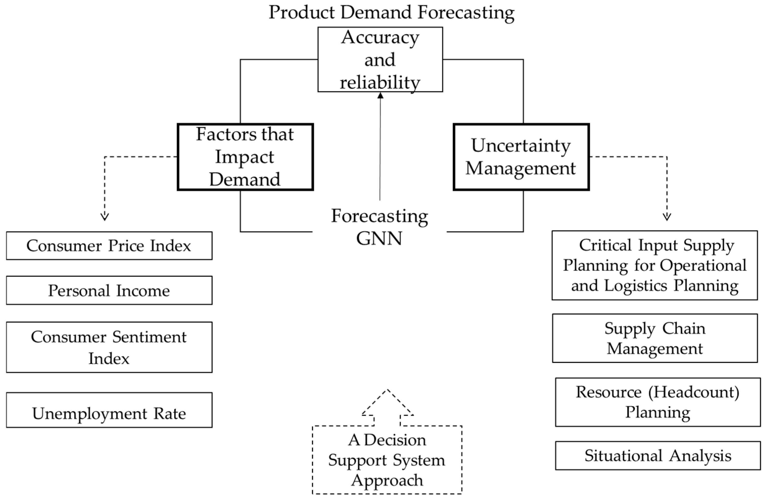
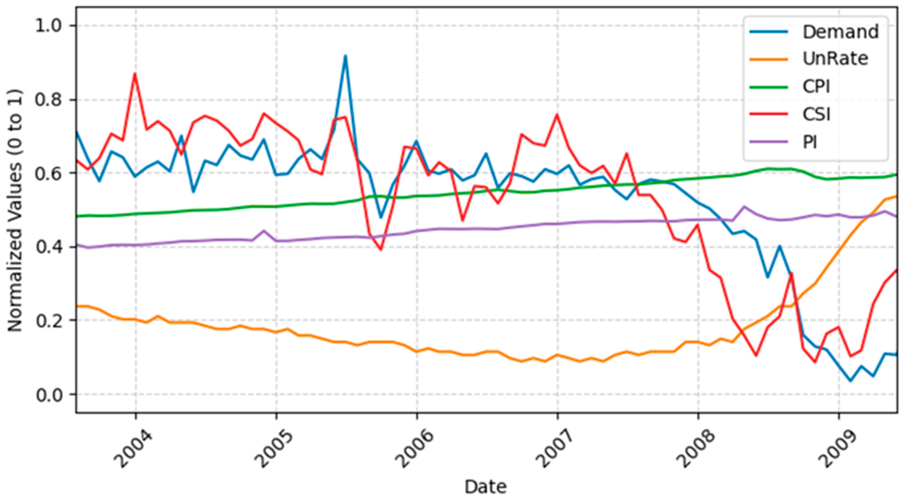
Figure 2 summarizes the three key components considered in this study: the factors that influence demand, the accuracy and reliability of the forecast, and the management of uncertainty. These elements help explain how demand forecasting is connected to both operational and strategic decisions within the DSS. Figure 3 shows a graph of the factors considered.

Demand Forecasting

Forecasting is an important component within DSSs. Its main function is to provide information about the future state of the process, which is vital for informed and efficient decision. The DSS uses forecasting for Input Supply Planning, Operational Planning, and Logistics Planning. Demand estimates serve as a primary input for effective planning and decision-making in departments such as marketing, production, distribution, and finance. Accurate forecasts help plan the correct combination of products to be acquired, resulting in significant savings in inventory and transportation costs [34].
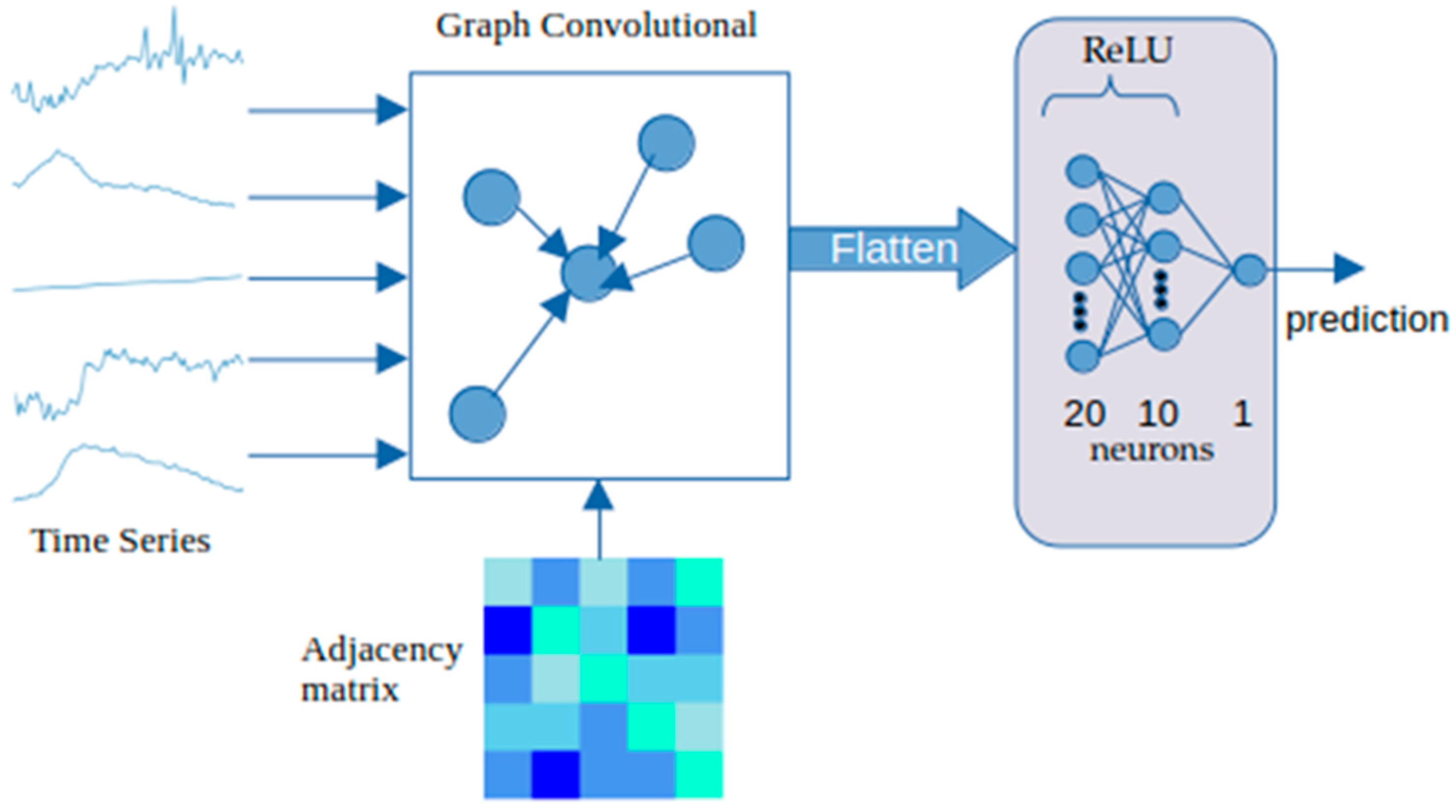
To perform the prediction within the module, we propose a new architecture based on GNNs. The graph is constructed to model the relationships between demand and the indices CSI, CPI, PI, and UnRate. Each node in the graph contains as features the historical data of its corresponding time series, while the edges include weights that capture the relationships between each index node and the demand node. To determine these edge weights, we used the feature importances obtained from an AdaBoost classifier. Figure 4 describes and formalizes the network.
The prediction module based on GNNs [35] is as follows. The structure is a graph G = V , E where the set of nodes V is defined by the demand time series and four macroeconomic indices. Thus, the number of nodes is N = 5 . The features for each node are their respective historical time series data, which form the input feature matrix X R N × T , where T is the length of the historical window. The edges E and their corresponding weights in the adjacency matrix A R N × N are crucial, since these weights quantify the relationship between the index nodes and the demand node. Specifically, the weights are determined by the feature importances derived from a pre-trained AdaBoost classifier, ensuring that the graph topology reflects the most salient economic drivers of demand.
The decision to use the feature importance derived from an AdaBoost Regressor as a proxy for the adjacency matrix weights, rather than a more conventional approach like correlation or mutual information, is primarily driven by the need to capture non-linear, predictive dependencies relevant to the forecasting task. Unlike simple correlation, which only measures linear relationships, AdaBoost inherently prioritizes features that contribute most effectively to minimizing the model’s loss function used for the forecasting task. This means that the derived importance score directly reflects how causally or functionally relevant one variable is to the prediction of another variable’s future value, an important requirement for time series forecasting. While methods like mutual information also capture non-linearities, the AdaBoost’s ensemble mechanism provides a more robust and smooth measure of importance, filtering out noise and focusing on consistent predictive power. Furthermore, this approach allows the graph structure to be inherently task-aware on forecasting and predictively optimized.
The architectural flow is as follows. The system receives the input feature matrix X , that is, the five-time series, and the adjacency matrix
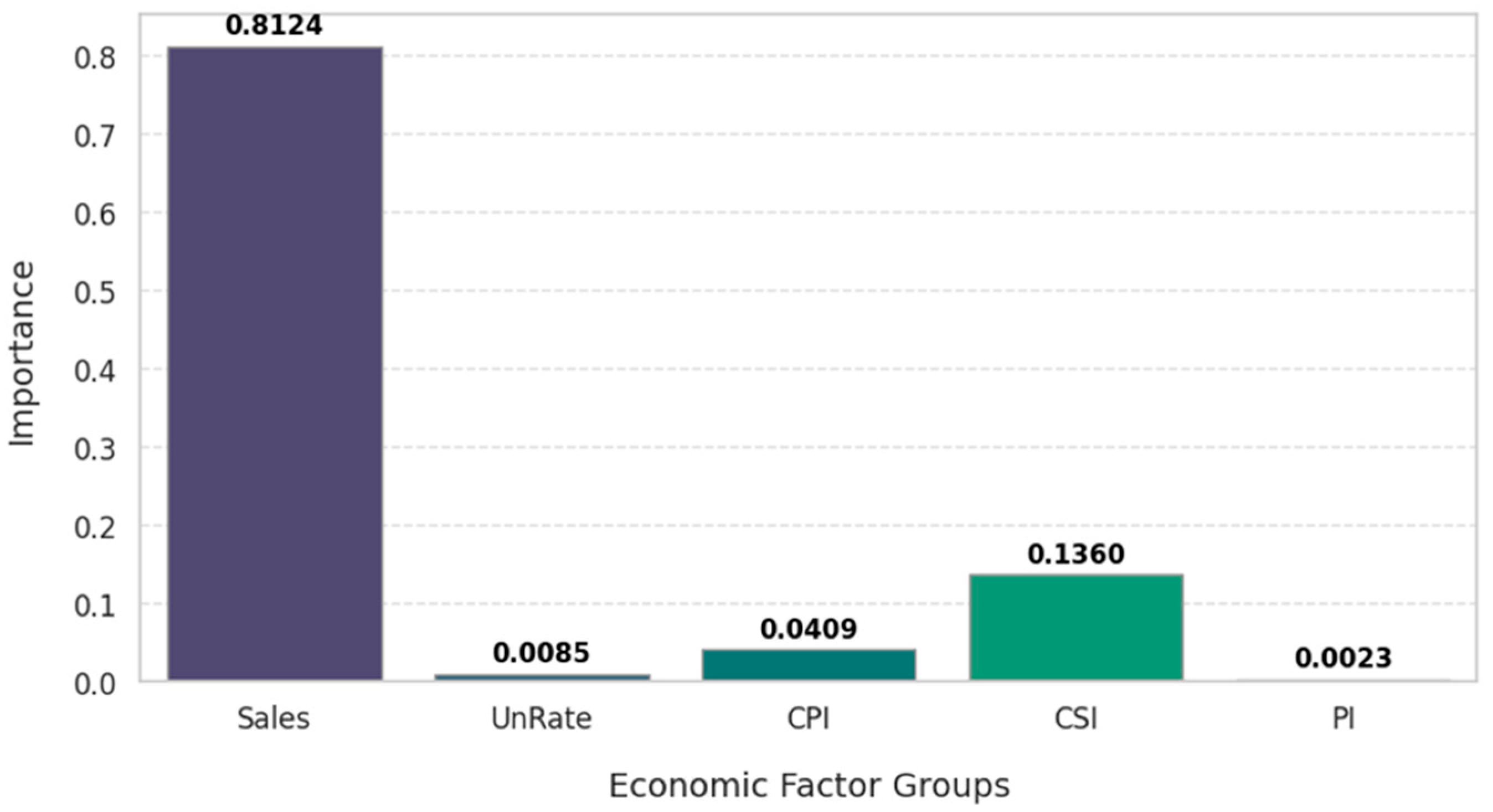
A = 0.8124 0.0085 0.0409 0.1360 0.0023 0.0085 0 0 0 0 0.0409 0 0 0 0 0.1360 0 0 0 0 0.0023 0 0 0 0
where we used the values of the feature importance calculated in the Results section. A Graph Convolutional Layer (GCL) processes the input to extract spatial and temporal features. We use F = 10 filters. The output H is calculated as
H = R e L U (   D 1 2 A ~ D 1 2 X W )
where A ~ = A + I is the adjacency matrix with self-connections, D is the degree matrix of A ~ , and W is the learnable weight matrix for the GCL.
The output of the GCL is vectorized before being fed into the fully connected layers.
z = F l a t t e n ( H )
The vector z is then processed by two successive fully connected or Dense layers, both employing the Rectified Linear Unit (ReLU) activation function
h 1   = R e L U ( z W ( 1 ) + b ( 1 ) )
h 2   = R e L U ( h 1 W ( 2 ) + b ( 2 ) )
where the first layer has 20 neurons W ( 1 ) R N F × 20 and the second has 10 neurons W ( 2 ) R 20 × 10 and b(2) is a bias factor. The final prediction y ^ is generated by a single neuron with a linear activation function:
y ^   = R e L U ( h 2 W ( 3 ) + b ( 3 ) )
where W ( 3 ) R 10 × 1 and y ^ is the predicted demand.

4.3. Decision Support System Components for Demand Forecasting

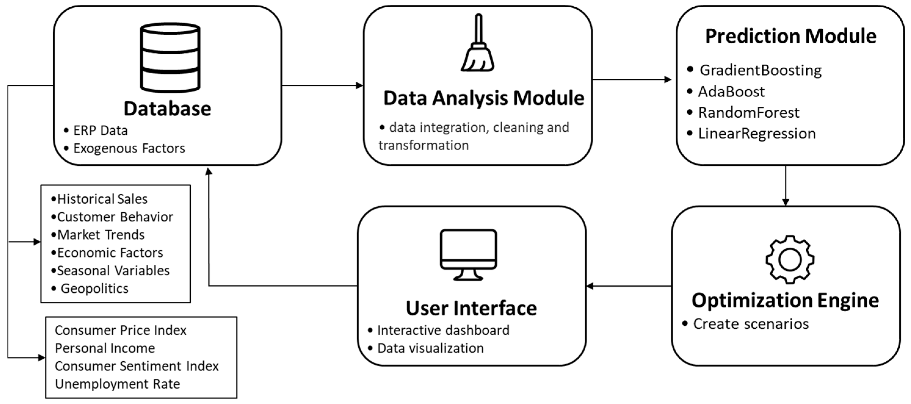
The integration of DSS in demand forecasting represents a significant leap forward, enabling real-time data analysis and informed decision-making [36]. A conceptual design for a DSS tailored to Industry 4.0 is presented, incorporating a variety of records and applies an all-encompassing approach to utilizing database-oriented information and analytical models [37]. To provide actionable information and support informed decision-making in a dynamic and competitive environment, the resulting framework is presented in Figure 5 and proposes the following DSS components for demand forecasting:
  • Intuitive User Interface: a user-friendly and visually clear interface is required to facilitate interaction and ensure users can easily understand the results.
  • Database: this represents the data repository used within the system. It stores and organizes the relevant information needed for the decision-making process. The database may be relational or multidimensional depending on system requirements. It contains historical and current data, as well as the parameters necessary for analysis and decision generation.
  • Data Analysis Modules: these modules enable data integration, cleaning, and transformation, as well as the identification of relevant patterns and trends. They may include regression models, time-series analyses, simulations, and others.
  • Prediction module: in this study, we evaluate the following algorithms: Gradient Boosting, AdaBoost, Random Forest, and Linear Regression. These Machine Learning algorithms (prediction module) are used to build predictive models based on historical data and relevant external variables.
  • Optimization Engine (decision-making module): responsible for generating recommendations and optimal scenarios based on analytical results and organizational objectives.

4.4. Integration Flow Between GNN and DSS

In this section we describe the integration of the prediction Module and the Optimization Engine. In our current implementation, the GNN produces a point forecast of future demand, denoted y ^ . This prediction is fed directly into the DSS’s optimization engine, which uses it to update key inventory control parameters, such as safety stock levels, reorder points, and order quantities. Although the GNN does not output predictive uncertainty, the DSS incorporates robustness through empirically derived safety margins, based on historical forecast errors or demand variability. The end-to-end integration flow is detailed below illustrated with a safety stock level scenario:
  • The GNN processes the item relationship graph and temporal covariates to generate a point forecast y ^ for each item.
  • Each forecast y ^ replaces the previous demand estimate in the DSS’s inventory model.
  • The optimization engine recomputes safety stock (SS) using a standard formula: S S = k · σ h i s t . Where σ h i s t is the historical standard deviation of demand or of past forecast errors for that item, and k is a service-level factor.
  • The reorder point (ROP) is updated as: R O P = y l e a d   t i m e + S S .
    where y l e a d   t i m e , the expected demand during the lead time, is the GNN forecast aggregated over the supplier lead time.
  • If the newly computed safety stock or reorder point differs from the current policy by more than a predefined threshold, e.g., ±10%, the DSS triggers a specific, actionable recommendation for example “Increase safety stock for Item X from 20 to 25 units”.
  • The user can review, simulate the financial or service-level impact, or approve the recommendation; outcomes are logged to support future model refinement.

5. Results

5.1. Results of Demand Forecasting

This section presents the results obtained in the demand forecasting task. For this, a sales series was used as a proxy for demand, this series represents monthly sales of light-weight vehicles, including automobiles and light trucks [38]. These data belong to the automotive and transportation sector and measure product units sold, expressed in millions at a seasonally adjusted annual rate. It serves as a macroeconomic indicator of vehicle demand and overall market activity. Additionally, the time series for the CSI, CPI, PI, and UnRate indices were obtained from databases [39,40,41,42], respectively. These data are summarized in Table 1, which presents the descriptive statistics of the variables used in the analysis.
The data used consists of 595 monthly observations. The series were divided using the sliding window method, with historical window length of T = 10, resulting in a total of 585 windows for each series. These were then concatenated into a tensor of size (585, 50), and each of the 585 windows also included the corresponding prediction value as target. The data were split into training and test sets, with 80% used for training and the remainder for testing. We used a temporal split, since this ensured that the model was strictly trained on past observations and evaluated only on subsequent, future data, thus preserving the integrity of the predictive task. The algorithms used for comparisons were Gradient Boosting, Ada Boost, Rando Forest, and Linear regression was used as a base line. All models were systematically tuned using Grid Search to ensure a fair comparison with our proposed model. For the Gradient Boosting Regressor, the number of boosting stages was optimized in steps of 20, resulting in an optimal value of 140. We trained this regressor using the squared error loss function and a fixed learning rate of 0.1. In the case of AdaBoost, the number of base estimators was also optimized in steps of 20, where 140 was found to be the best value, and a linear loss function was utilized for training. Finally, for the Random Forest Regressor, the number of trees was determined to be 100 after optimization via Grid Search in steps of 20, and the squared error criterion was used to measure the quality of a split. For training the proposed model, we utilized the Adaptive Moment Estimation (Adam) algorithm for optimization, employing the mean absolute error as the loss function. The training was executed over 700 epochs with a batch size of 15. No additional explicit regularization techniques were applied during training.
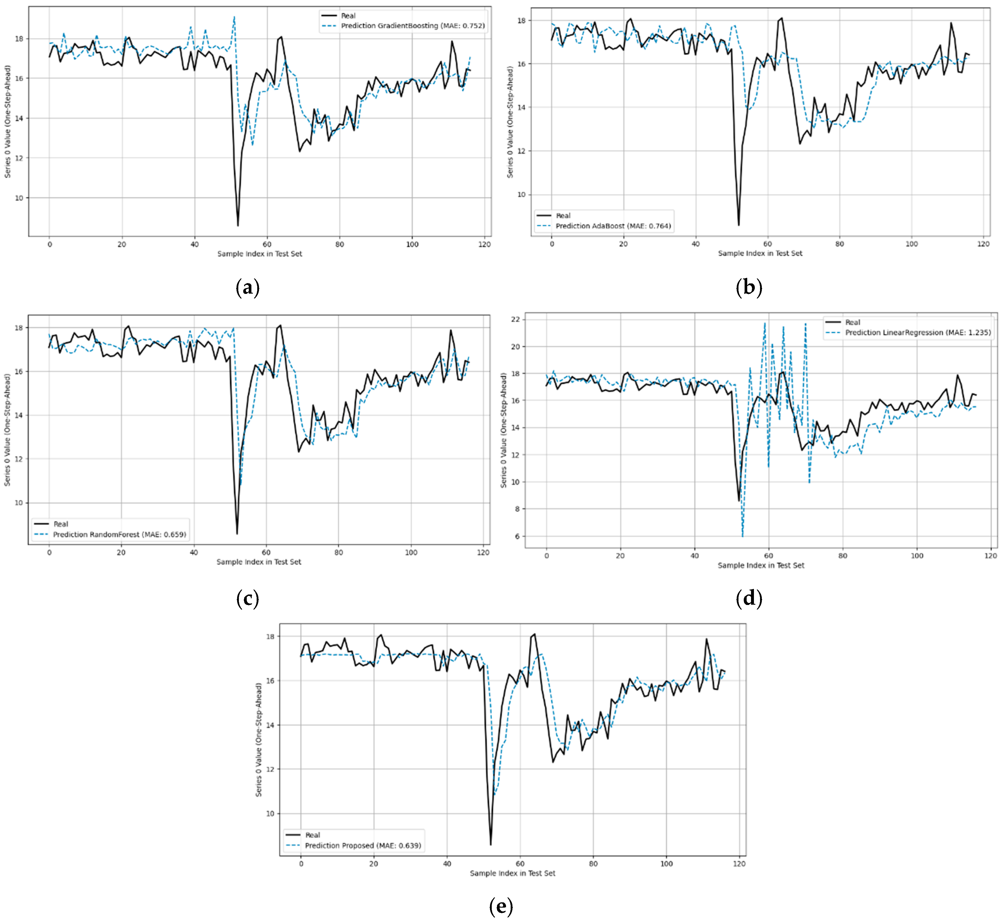
The performance of the algorithms for time series forecasting is shown in Table 2 and Figure 6. Only the proposed model and AdaBoost partially follow the sudden change observed in Figure 6, while Gradient Boosting and Random Forest tend to over-smooth the transition, failing to capture the sharp jump. This suggests that the proposed model, by incorporating relationships with external series, is more sensitive to points where the underlying dynamics change abruptly.
On the other hand, Linear Regression shows the weakest performance, as shown both in the metrics (with a negative R2 and a substantially higher MSE) and in the plot, where its predictions diverge significantly from the true series. This result indicates that the relationship between the variables and demand is not linear, and that the series exhibits patterns such as seasonality, irregularity, or nonlinear interactions that a linear model cannot capture.
In contrast, tree-based and ensemble methods demonstrate greater flexibility to adapt to complex relationships, which explains their superior performance in this context.
The results of Table 2 confirm the effectiveness of the proposed GCN-based model, achieving an MAE of 0.63, the lowest among all evaluated methods. The performance of the proposed model is comparable to that of Random Forest (MAE 0.65), also it achieves an improvement in explained variance, with a value of 0.57 compared to 0.55. Techniques like AdaBoost and Linear Regression showed less performance, with MAEs of 0.8 and 1.2, respectively, and negligible or negative explanatory capacity in the case of Linear Regression.
To validate results of Table 2, we employed the Diebold-Mariano (DM) test on the forecast errors using the MAE loss function. The results confirm that the proposed GCN-based model is statistically superior to all traditional benchmark models at the alpha = 0.05 significance level. Specifically, the DM test yielded highly significant p-values when comparing the proposed model against Gradient Boosting (p < 0.0001, DM = −6.8411), AdaBoost (p < 0.0001, DM = −6.9736), and Linear Regression (p < 0.0001, DM = −10.8718). The proposed model also demonstrated statistically significant superiority over the competitive Random Forest model (p = 0.0288, DM = −2.2131).
To more closely validate the response of the algorithms to abrupt changes in the demand we calculate the error on these samples. We characterize an abrupt change if the following condition is met
Δ y t = y t y t 1 > k · σ Δ y
where y t is the value of the series at sample t, Δ y t is the change at sample t, σ Δ y = 0.4 s the standard deviation in the time series segment, and k = 5 is a constant, these values were determined empirically.
From Figure 6, it can be observed that most methods fit the data reasonably well in stable intervals or those with smooth variations. However, in abrupt transitions such as the one occurring around sample index 6 the models differ notably in their responsiveness.
Table 3 presents the absolute prediction error across four distinct demand samples (Samples 51, 52, 53, and 63) with abrupt changes Δ y t > k · σ Δ y .
The results reveal significant performance variations across samples. Notably, the proposed model achieves the lowest error in Samples 51 and 63 (5.2 and 1.8, respectively) and performs competitively in the others, demonstrating its robust adaptability. In contrast, traditional methods show inconsistent performance; for instance, Linear Regression yields the highest error in Sample 53 (6.3), while Gradient Boosting performs best in Sample 53 (1.1) but poorly in Sample 51 (7.7). This sample-wise analysis underscores that the proposed model offers more stable and accurate demand predictions overall. The primary enhancement of the proposed GCN approach lies in its ability to accurately capture ‘abrupt changes’ and high-volatility segments in demand, which traditional baseline models often fail to detect due to excessive smoothing. For decision-makers, this capability is important as it enables a more responsive supply chain that can preemptively adjust inventory levels, thereby minimizing the financial risks associated with both backorders during sudden demand spikes and high storage costs during unexpected drops.
Additionally, as stated in Section 4, the adjacency matrix weights used to model the relationship between factors were determined by feature importance scores derived from a pre-trained AdaBoost model. This analysis was conducted to quantify the dependencies among the considered factors and integrate these values into the graph structure. Figure 7 illustrates the incorporated factors along with numerical values representing the relative contribution. The model’s feature importance ranking was led by the historical demand series (8.81), capturing core time-series patterns. It was meaningfully supported by economic indicators: Consumer Sentiment Index (0.13) and Consumer Price Index (0.04). The Unemployment Rate (0.0085) and Personal Income (0.0023) had marginally direct impacts, with the latter’s effect likely absorbed by other correlated factors.
Additionally, we conducted a brief ablation study on a reduced subset of the test set and all training using 100 epochs. This study involved replacing the Graph Convolutional Layer with either a standard Dense layer (50 neurons, ReLU) or a 1D Convolutional (CNN) layer with 10 filters. The baseline GCN with F = 10 achieved a MAE of 1.8, outperforming not only the simpler Dense and CNN models, which yielded MAEs of 16.8 and 11.4 respectively, but also the hyperparameter variations using F = 16, MAE 18.6, and F = 4, MAE 3.8. This empirical evidence justifies the selection of F = 10 for this specific dataset and model configuration.
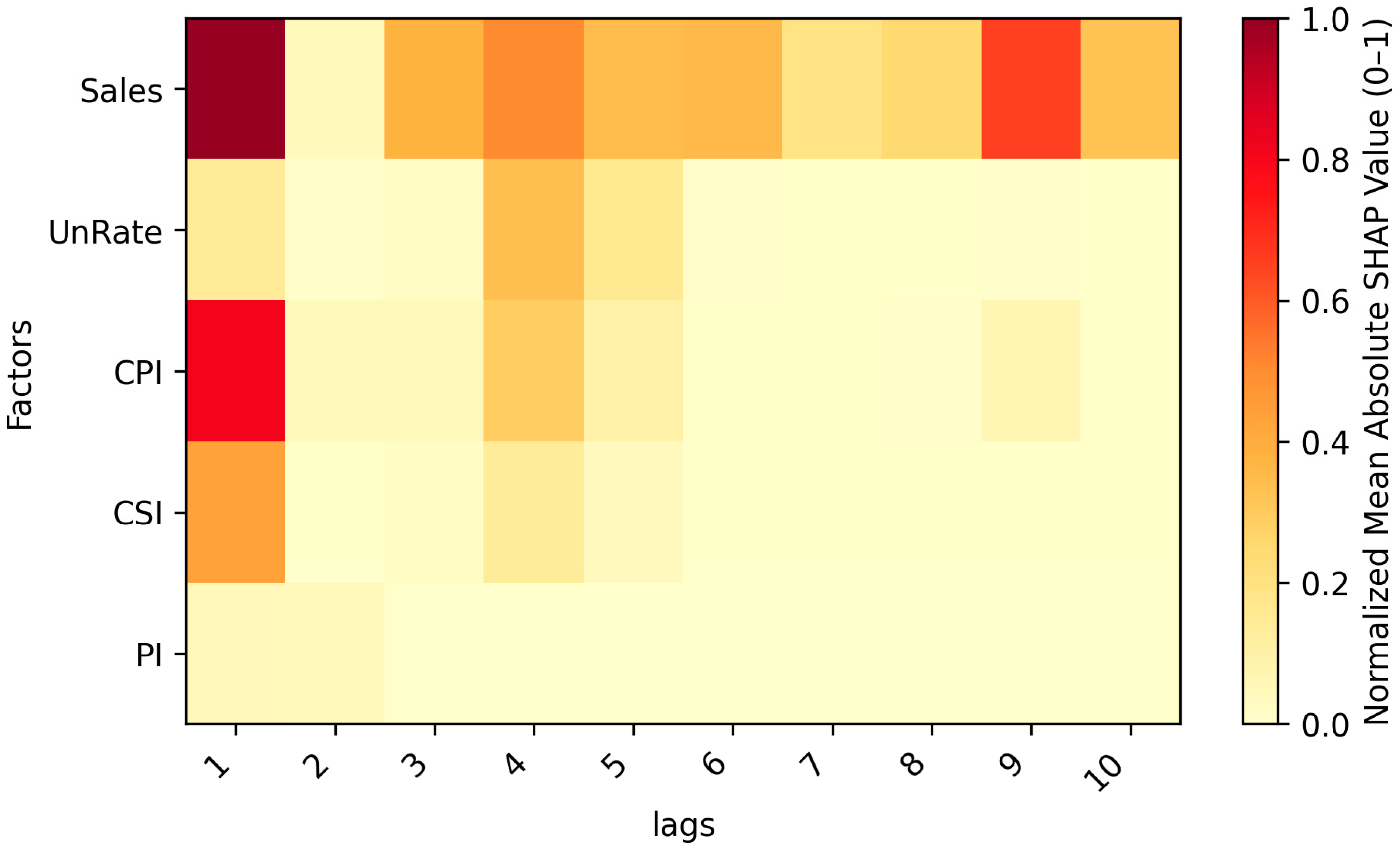
We performed a SHAP (SHapley Additive exPlanations) analysis to quantify the contribution of each input factor to the GCN’s final predictions. This analysis helps to identify which external variables provide the greatest informational value to the model and, therefore, which should be monitored more closely to support strategic decision-making. The results are summarized in Figure 8 that shows a normalized average importance matrix, where the rows correspond to the factors (Sales, UnRate, CPI, CSI, PI) and the columns represent the lags of the window time series used for the forecast. The analysis reveals that the Sales series itself and its corresponding lags are the most important inputs, for the model’s decision process with a normalized maximum importance of 1.0 at lag 1 and high values across multiple past observations. The CPI and CSI factors also show significant impact, especially at short-term lags. Conversely, the PI factor and most of the long-term lags across all other macroeconomic variables contribute minimally, suggesting the GCN primarily relies on recent past Sales data and the immediate state of the CPI and CSI to predict future demand.

5.2. Managerial Implications of Demand Forecasting with a Proposed DSS

The implementation of the DSS and the demand forecasting framework developed in this study have direct implications for managerial decision-making within the supply chain. The accuracy achieved by the proposed model translates into measurable advantages that impact both tactical and operational planning. The system directly addresses the issue of imprecise information and inadequate forecasting methods [43].
The improvements observed in Section 4.1, particularly the lower MAE and MSE achieved by the proposed model compared to tree-based and linear baselines, have direct managerial implications for inventory and production planning. Lower forecast errors reduce uncertainty in demand estimates, which in operational terms allows decision-makers to adjust safety stock levels more accurately. For example, a consistent reduction in average forecasting error implies narrower confidence intervals around demand projections, enabling firms to maintain lower buffer inventories while preserving service levels. Similarly, the improved ability of the model to react to abrupt demand changes, as illustrated in Figure 6, supports faster corrective actions in production and replenishment decisions, reducing the risk of delayed responses to market variability.
In operational and tactical planning, accurately forecasting future demand is essential for supply chain management, as it impacts key decisions related to planning and inventory control. The DSS enables managers to translate demand time-series predictions into actionable decisions, in areas such as the following:
Inventory optimization and cost reduction (structured decision): Since precise replenishment recommendations help prevent operational inefficiencies caused by inaccurate forecasts. By calculating the optimized inventory level, the DSS minimizes costs associated with both overstock and stockouts, while reducing risks such as increased backorders or higher storage costs. This contributes to the overall objective of reducing inventory levels and improving forecast accuracy, resulting in significant financial savings [44].
Production planning and resource allocation: With accurate forecasts, firms can avoid overproduction, reduce stockouts, optimize the use of materials and equipment, and ensure that resources are allocated where they are most needed, ultimately improving operational efficiency and reducing costs.
In strategic alignment and market adaptation, the DSS could provide a structured framework for data analysis, scenario modeling, and evaluation of decision alternatives. The results and sensitivity analysis functionalities enable the Situational Analysis needed for strategic decision-making.
Additionally, the DSS could help in the identification of the relative importance of factors. Since sensitivity analysis helps identify which factors, e.g., historical sales, market trends, seasonal variables that can have influence on predicted demand. This insight guides future investment in data quality and improves the level of data integration in order for the decision-making process remains accurate, informed, and efficient [45].

5.3. Scenario Visualization in the DSS: Conceptual Dashboard

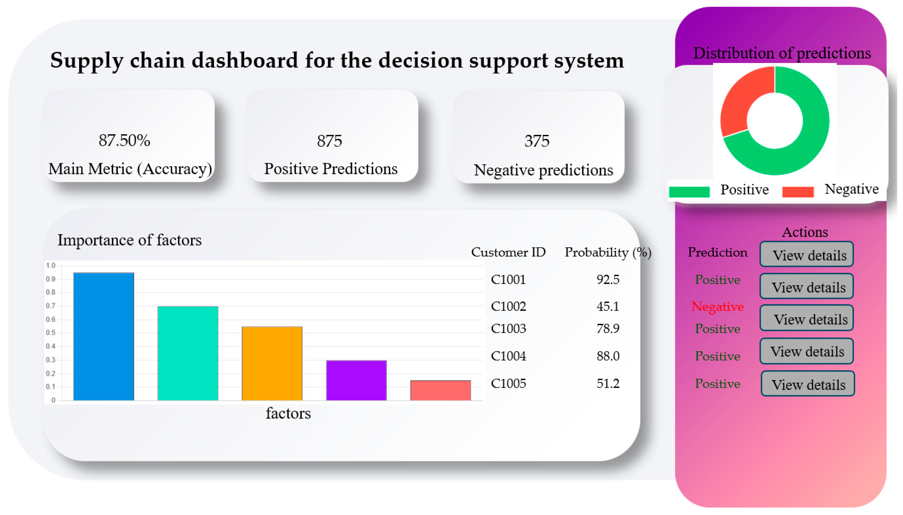
To illustrate how the DSS translates predictions into operational decisions, a conceptual dashboard was developed to represent the output of the decision module. The scenarios displayed in this dashboard are conceptually grounded on the trained GNN-based forecasting model, where controlled perturbations of selected input features are used to analyze their impact on demand predictions. This visualization does not use real operational data; instead, it illustrates the system’s behavior under different market conditions by propagating modified input values (e.g., changes in CSI) through the trained model, following the methodology described in Section 3.3 and the simulation framework introduced in Section 3.2. The dashboard includes the following elements:
  • Model performance metrics: overall accuracy, number of positive predictions, and number of negative predictions.
  • Importance of external factors: a bar chart showing the relevance of variables such as CSI, CPI, PI, and UnRate in demand prediction.
  • Prediction distribution: a donut chart that displays the proportion of positive and negative decisions.
  • Customer-level probability table: segmentation of decisions by customer ID and associated probability level.
  • Action buttons: allow users to simulate decisions such as increasing production, adjusting inventory, or reviewing critical customers.
Figure 9 shows the conceptual DSS dashboard designed to support structured and semi-structured decision-making in dynamic environments. The primary users of the proposed DSS dashboard are supply chain planners, operations managers, and manufacturing engineering managers operating at tactical and operational levels. The system is designed for medium-to-large manufacturing and distribution companies that face demand volatility and rely on data-driven planning for inventory control, production scheduling, and resource allocation. In this context, the dashboard serves as a decision interface that translates model-based demand forecasts into actionable insights, supporting structured decisions such as replenishment planning and semi-structured decisions such as production adjustments under changing market conditions.
This tool enables DSS users to visually explore scenarios derived from perturbations of key exogenous variables within the GNN model, as defined in the simulation experiments:
  • Optimistic scenario: an increase in the CSI input is introduced to the trained GNN, resulting in higher predicted demand and triggering recommendations to ramp up production.
  • Pessimistic scenario: a decrease in the CSI input leads the model to forecast lower demand, suggesting production slowdown and tighter inventory control.
  • Baseline scenario: original input values are maintained, providing a reference forecast against which deviations in alternative scenarios can be compared.
The conceptual dashboard developed as part of the DSS serves as a visual interface for strategic and operational decision-making in supply chain management. By integrating prediction probabilities per customer, the distribution of positive and negative decisions, and the relative importance of external factors such as the CSI, CPI, PI, and UnRate the system enables scenario simulation and anticipatory planning. This visualization supports risk identification, production adjustment, and inventory optimization, reinforcing the DSS as a robust tool for navigating economic volatility and enhancing demand forecasting accuracy.

6. Conclusions and Future Works

This study proposes and evaluates a DSS for demand forecasting based on a GNN architecture that integrates macroeconomic indicators and historical demand data. The results demonstrate that the proposed model outperforms traditional machine learning methods, particularly in scenarios involving abrupt changes or nonlinear dynamics in the demand series. The findings confirm that representing exogenous variables within a graph structure enhances predictive accuracy and provides actionable insights for decision-makers.
From a managerial perspective, the proposed DSS supports operational, tactical, and strategic decision-making by improving demand forecasting accuracy and reducing uncertainty in planning processes. The experimental results show that the proposed GNN-based method achieves the lowest MAE (0.64) outperforming all methods used in the comparison. Specifically, it improves upon Random Forest (0.66), Gradient Boosting (0.75), AdaBoost (0.76), and Linear Regression (1.23). This improvement in MAE highlights the effectiveness of the proposed approach in capturing the underlying demand patterns more accurately, leading to more reliable point forecasts.
The accuracy improvements translate into tangible managerial benefits, including more reliable replenishment planning, reduced inventory holding costs, and better alignment between production and actual market demand. In particular, the reduction in forecasting error enables decision-makers to anticipate demand fluctuations more effectively, supporting scenario-based planning and risk mitigation strategies.
Consequently, the integration of GNN-based forecasting within the DSS enhances operational efficiency, improves responsiveness to market changes, and supports informed strategic decisions in dynamic and uncertain environments.
In alignment with the core themes of future internet, this study shows how intelligent digital systems, data analytics, and AI-driven forecasting models contribute to the development of smart supply chains. As industrial environments continue to adopt interconnected digital infrastructures, the integration of advanced predictive algorithms within DSS platforms will be essential for achieving resilience, adaptability, and efficiency.
Future research may extend the model toward real-time forecasting using streaming data, integration with IoT-based sensing systems, or the development of full intelligent supply-chain ecosystems where data, decisions, and human oversight operate seamlessly within the broader framework of the future internet.
Additionally, future studies will analyze the sensitivity of the proposed model to different types of exogenous variables, such as macroeconomic indicators, policy changes, and market disruptions, in order to improve robustness and adaptability. Finally, the integration of explainable artificial intelligence techniques will improve transparency and trust in the model’s recommendations, enabling decision-makers to better understand the rationale behind forecasts and to assess their impact on operational and strategic planning.

Author Contributions

Conceptualization, S.S.-D. and J.-M.M.-M.; methodology, J.-M.M.-M., S.S.-D. and O.C.-M.; software, J.-M.M.-M. and L.O.-M.; validation, O.C.-M. and J.-M.M.-M.; investigation, S.S.-D., J.-M.M.-M., R.P.-G., A.-S.D.-F., L.O.-M. and O.C.-M.; data curation, J.-M.M.-M.; writing—original draft preparation, S.S.-D. and J.-M.M.-M.; writing—review and editing, R.P.-G., A.-S.D.-F., and O.C.-M.; supervision, J.-M.M.-M. All authors have read and agreed to the published version of the manuscript.

Funding

This research received no external funding.

Data Availability Statement

Data are derived from public domain resources. The data presented in this study are available in FRED at https://fred.stlouisfed.org/ (accessed on 25 November 2025). These data were derived from the following resources available in the public domain: https://fred.stlouisfed.org/.

Acknowledgments

This work was made possible thanks to the infrastructure and institutional support provided by the Universidad Autónoma de Ciudad Juárez (UACJ). We extend our gratitude to SECIHTI for its continued dedication to fostering academic advancement and research initiatives, which played an essential role in completing this study. We declare the use of AI, for grammar and spelling review. The methodology, analysis, originality, validity, and integrity were carried out exclusively by the authors. No AI was used for such a purpose.

Conflicts of Interest

The authors declare no conflicts of interest.

Abbreviations

The following abbreviations are used in this manuscript:
DSSDecision Support System
GNNGraph Neural Networks
CSIConsumer Sentiment Index
CPIConsumer Price Index
PIPersonal Income
UnRateUnemployment Rate
IoTInternet of Things

References

  1. Seyedan, M.; Mafakheri, F. Predictive big data analytics for supply chain demand forecasting: Methods, applications, and research opportunities. J. Big Data 2020, 7, 53. [Google Scholar] [CrossRef]
  2. Gonçalves, J.N.C.; Cortez, P.; Carvalho, M.S.; Frazão, N.M. A multivariate approach for multi-step demand forecasting in assembly industries: Empirical evidence from an automotive supply chain. Decis. Support Syst. 2021, 142, 113452. [Google Scholar] [CrossRef]
  3. Badr, H.; Ahmed, W. A Comprehensive Analysis of Demand Prediction Models in Supply Chain Management. AJIBM 2023, 13, 1353–1376. [Google Scholar] [CrossRef]
  4. Tadayonrad, Y.; Ndiaye, A.B. A new key performance indicator model for demand forecasting in inventory management considering supply chain reliability and seasonality. Supply Chain Anal. 2023, 3, 100026. [Google Scholar] [CrossRef]
  5. Aldahmani, E.; Alzubi, A.; Iyiola, K. Demand Forecasting in Supply Chain Using Uni-Regression Deep Approximate Forecasting Model. Appl. Sci. 2024, 14, 8110. [Google Scholar] [CrossRef]
  6. Christopher, M. Logistics and Supply Chain Management; Pearson: London, UK, 2022; ISBN 978-1-292-41619-9. [Google Scholar]
  7. Zambrano-Ponce, A.; Zaldumbide-Peralvo, D. Disponibilidad de inventarios frente a la demanda en productos de Tiendas TuTi. 593 Digit. Publ. CEIT 2024, 9, 228–244. [Google Scholar] [CrossRef]
  8. Palafox-Palafox, D.; Medina-Marín, J.; Seck-Tuoh-Mora, J.C.; Serna-Díaz, M.G.; Hernández-Romero, N. Modelo de pronóstico de cadena de suministro mediante redes neuronales. Pädi Boletín Científico De Cienc. Básicas E Ing. Del ICBI 2023, 11, 103–111. [Google Scholar] [CrossRef]
  9. Calle García, J.S.; Pincay Delgado, M.A.; Mendoza Pionce, B.S.; Bravo Quijije, G.S. USO ESTRATÉGICO DE LA INTELIGENCIA ARTIFICIAL EN LA GESTIÓN DE LA CADENA DE SUMINISTRO EMPRESARIAL. Cien. Y Des. 2024, 27, 267. [Google Scholar] [CrossRef]
  10. Sebastian, J.; Riascos-Guerrero, J.A.; Galván-Colonia, E.; Pincay-Lozada, J.L. Estrategias basadas en inteligencia artificial para la gestión de inventarios en la cadena de suministro. Rev. Tecnol. En Marcha 2024, ág, 88–97. [Google Scholar] [CrossRef]
  11. Teniwut, W.A.; Hasyim, C.L. Decision support system in supply chain: A systematic literature review. Uncertain Supply Chain. Manag. 2020, 8, 131–148. [Google Scholar] [CrossRef]
  12. Bron Fonseca, B.; Mar Cornelio, O. Sistemas De Recomendación Para La Toma De Decisiones. ESTADO Del Arte: Sistemas De Recomendación Para La Toma De Decisiones. UNESUM-Cienc. 2022, 6, 149–164. [Google Scholar] [CrossRef]
  13. Avdeeva, Z.; Kovriga, S.; Fedko, E. DSS-Tool for Demand Planning: An Example of Automotive Industry. In Proceedings of the 2019 IEEE 21st Conference on Business Informatics (CBI), Moscow, Russia, 15–17 July 2019; pp. 51–59. [Google Scholar]
  14. Marco, G.; Silva, F.; Ferraz, F.; Silva, A.; Analide, C.; Novais, P. Developing an ambient intelligent-based decision support system for production and control planning. In Proceedings of the International Conference on Intelligent Systems Design and Applications, Porto, Portugal, 16–18 December 2016; Springer International Publishing: Cham, Switzerland, 2016; pp. 984–994. [Google Scholar]
  15. Fadda, E.; Perboli, G.; Rosano, M.; Mascolo, J.E.; Masera, D. A Decision Support System for Supporting Strategic Production Allocation in the Automotive Industry. Sustainability 2022, 14, 2408. [Google Scholar] [CrossRef]
  16. Sauer, C.R.; Burggräf, P.; Steinberg, F. A systematic review of machine learning for hybrid intelligence in production management. Decis. Anal. J. 2025, 15, 100574. [Google Scholar] [CrossRef]
  17. De Lima, D.; Corso, L.L. Aplicação de Inteligência Artificial e Modelos Matemáticos para Previsão de Demanda em uma indústria do ramo plástico. Sci. Cum Ind. 2020, 8, 24–29. [Google Scholar] [CrossRef]
  18. Kilimci, Z.H.; Akyuz, A.O.; Uysal, M.; Akyokus, S.; Uysal, M.O.; Atak Bulbul, B.; Ekmis, M.A. An Improved Demand Forecasting Model Using Deep Learning Approach and Proposed Decision Integration Strategy for Supply Chain. Complexity 2019, 2019, 9067367. [Google Scholar] [CrossRef]
  19. Chen, C.-S.; Chen, Y.-J. Optimizing Supply Chain Networks with the Power of Graph Neural Networks. arXiv 2025. [Google Scholar] [CrossRef]
  20. Niu, T.; Zhang, H.; Yan, X.; Miao, Q. Intricate Supply Chain Demand Forecasting Based on Graph Convolution Network. Sustainability 2024, 16, 9608. [Google Scholar] [CrossRef]
  21. Chen, H.; Rossi, R.A.; Mahadik, K.; Eldardiry, H. A Context Integrated Relational Spatio-Temporal Model for Demand and Supply Forecasting. arXiv 2020. Available online: https://www.semanticscholar.org/paper/A-Context-Integrated-Relational-Spatio-Temporal-for-Chen-Rossi/82a9072ef6cf2209fc1216e635eca93d11e253e7 (accessed on 12 December 2025).
  22. Cini, A.; Marisca, I.; Bianchi, F.M.; Alippi, C. Scalable Spatiotemporal Graph Neural Networks. arXiv 2022. [Google Scholar] [CrossRef]
  23. Olatunji, A.O. Leveraging Data Science for Demand Forecasting and Inventory Management: A Comprehensive Review. J. Basic Appl. Res. Int. 2025, 31, 29–38. [Google Scholar] [CrossRef]
  24. Haque, M.S. Retail Demand Forecasting Using Neural Networks and Macroeconomic Variables. JMSS 2023, 4, 1–6. [Google Scholar] [CrossRef]
  25. Verstraete, G.; Aghezzaf, E.-H.; Desmet, B. A leading macroeconomic indicators’ based framework to automatically generate tactical sales forecasts. Comput. Ind. Eng. 2020, 139, 106169. [Google Scholar] [CrossRef]
  26. Sagaert, Y.R.; Aghezzaf, E.-H.; Kourentzes, N.; Desmet, B. Tactical sales forecasting using a very large set of macroeconomic indicators. Eur. J. Oper. Res. 2018, 264, 558–569. [Google Scholar] [CrossRef]
  27. Veena, S.; Aravindhar, J. Challenges of Machine Learning Algorithms Used in Business for Decision-Making; Social Science Research Network: Rochester, NY, USA; p. 5066812. [CrossRef]
  28. Laudon, K.C.; Laudon, K.; Laudon, J.P.; Traver, C.G. Essentials of Management Information Systems; Pearson: London, UK, 2023; ISBN 978-1-292-45036-0. [Google Scholar]
  29. Phillips-Wren, G.; Daly, M.; Burstein, F. Reconciling business intelligence, analytics and decision support systems: More data, deeper insight. Decis. Support Syst. 2021, 146, 113560. [Google Scholar] [CrossRef]
  30. Alahmadi, D.H.; Jamjoom, A.A. Decision support system for handling control decisions and decision-maker related to supply chain. J. Big Data 2022, 9, 114. [Google Scholar] [CrossRef]
  31. Oukhay, F.; Zaraté, P.; Romdhane, T. Intelligent Decision Support System for Updating Control Plans. arXiv 2020. [Google Scholar] [CrossRef]
  32. Barnes, M.L.; Olivei, G.P. The Forecasting Power of Consumer Attitudes for Consumer Spending. Working Papers, Working Paper 14-10. 2014. Available online: https://www.econstor.eu/handle/10419/109703 (accessed on 16 December 2025).
  33. Nguyen, T.N.; Haider, M.; Jisan, A.H.; Raju, M.A.H.; Imam, T.; Khan, M.M.; Jafar, A.E. Product Demand Forecasting with Neural Networks and Macroeconomic Indicators: A Comparative Study among Product Categories. J. Bus. Manag. Stud. 2024, 6, 170–175. [Google Scholar] [CrossRef]
  34. Douaioui, K.; Oucheikh, R.; Benmoussa, O.; Mabrouki, C. Machine Learning and Deep Learning Models for Demand Forecasting in Supply Chain Management: A Critical Review. Appl. Syst. Innov. 2024, 7, 93. [Google Scholar] [CrossRef]
  35. Kipf, T.N.; Welling, M. Semi-Supervised Classification with Graph Convolutional Networks. arXiv 2016. [Google Scholar] [CrossRef]
  36. Bousdekis, A.; Lepenioti, K.; Apostolou, D.; Mentzas, G. A Review of Data-Driven Decision-Making Methods for Industry 4.0 Maintenance Applications. Electronics 2021, 10, 828. [Google Scholar] [CrossRef]
  37. Hossain, M.A.; Tiwari, A.; Saha, S.; Ghimire, A.; Imran, M.A.U.; Khatoon, R. Applying the Technology Acceptance Model (TAM) in Information Technology System to Evaluate the Adoption of Decision Support System. J. Comput. Commun. 2024, 12, 242–256. [Google Scholar] [CrossRef]
  38. U.S. Bureau of Economic Analysis. Light Weight Vehicle Sales: Autos and Light Trucks [ALTSALES], Retrieved from FRED, Federal Reserve Bank of St. Louis. Available online: https://fred.stlouisfed.org/series/ALTSALES (accessed on 25 November 2025).
  39. U.S. Bureau of Labor Statistics. Consumer Price Index for All Urban Consumers: All Items in U.S. City Average [CPIAUCSL], 582 Retrieved from FRED, Federal Reserve Bank of St. Louis. Available online: https://fred.stlouisfed.org/series/CPIAUCSL (accessed on 25 November 2025).
  40. U.S. Bureau of Economic Analysis. Real Disposable Personal Income [DSPIC96], Retrieved from FRED, Federal Reserve Bank of 584 St. Louis. Available online: https://fred.stlouisfed.org/series/DSPIC96 (accessed on 25 November 2025).
  41. U.S. Bureau of Labor Statistics. Unemployment Rate [UNRATE], Retrieved from FRED, Federal Reserve Bank of St. Louis. Available online: https://fred.stlouisfed.org/series/UNRATE (accessed on 25 November 2025).
  42. University of Michigan: Consumer Sentiment [UMCSENT], Retrieved from FRED, Federal Reserve Bank 587 of St. Louis. Available online: https://fred.stlouisfed.org/series/UMCSENT (accessed on 25 November 2025).
  43. Jahin, M.A.; Shahriar, A.; Amin, M.A. MCDFN: Supply chain demand forecasting via an explainable multi-channel data fusion network model. Evol. Intell. 2025, 18, 66. [Google Scholar] [CrossRef]
  44. Ahmadov, Y.; Helo, P. Deep learning-based approach for forecasting intermittent online sales. Discov. Artif. Intell. 2023, 3, 45. [Google Scholar] [CrossRef]
  45. Ahmad, S. Machine Learning for Demand Forecasting in Supply Chain Optimization. preprint 2025. [Google Scholar] [CrossRef]
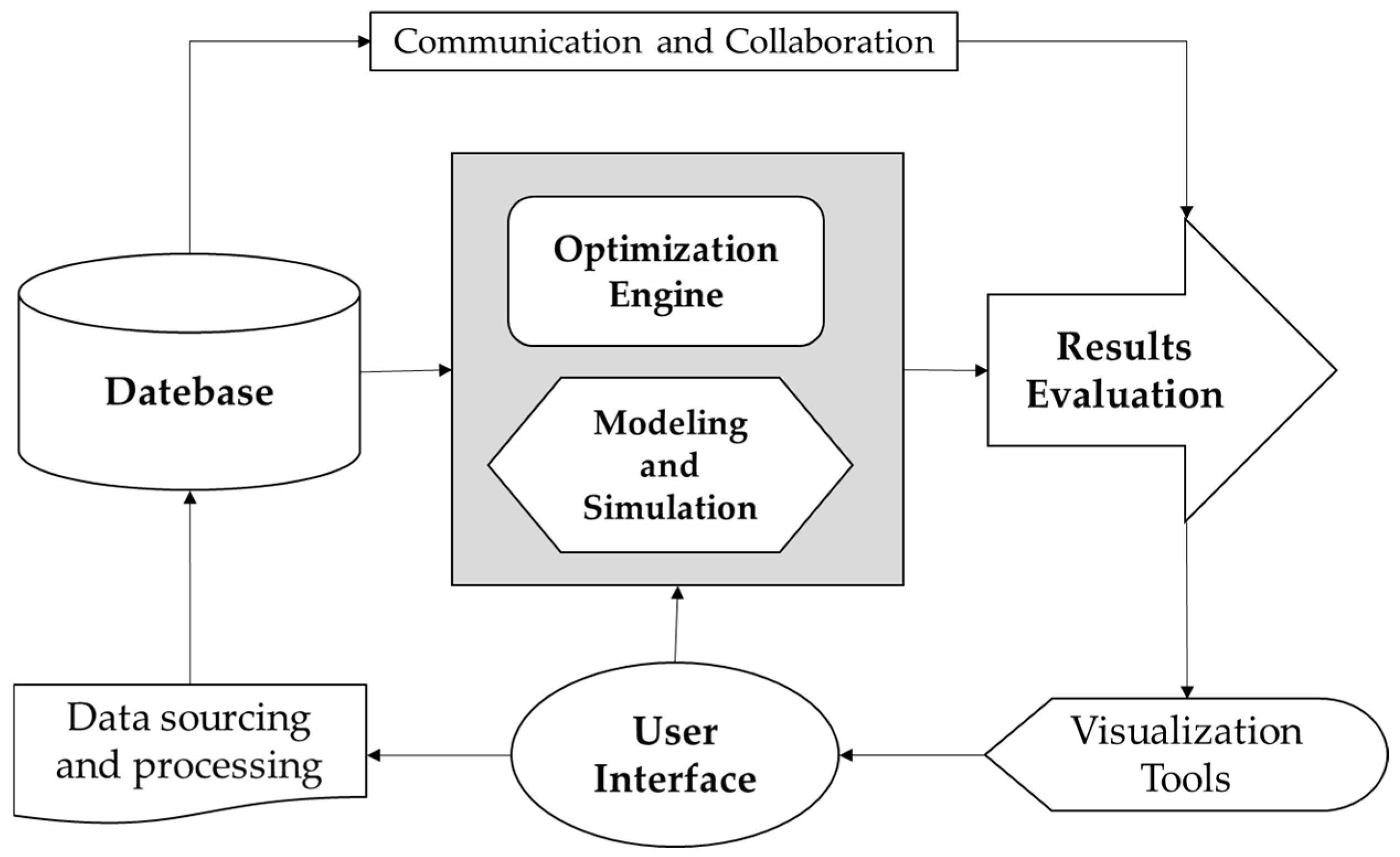
Figure 1. Architecture of a Decision Support System.
Futureinternet 18 00026 g001
Figure 2. Importance of the forecast in the proposed DSS.
Futureinternet 18 00026 g002
Figure 3. Sample time series of the factors considered.
Futureinternet 18 00026 g003
Figure 4. Proposed network for demand forecasting.
Futureinternet 18 00026 g004
Figure 5. Decision Support System for demand forecasting.
Futureinternet 18 00026 g005
Figure 6. Demand forecasting results. (a) GradientBoosting; (b) Adaboost; (c) RandomForest; (d) LinearRegression; (e) Proposed.
Futureinternet 18 00026 g006
Figure 7. AdaBoost feature importances.
Futureinternet 18 00026 g007
Figure 8. SHAP Feature Importance Map Normalized average contribution of each factor (row) and time lag (column) to the model’s prediction.
Futureinternet 18 00026 g008
Figure 9. Conceptual DSS dashboard for demand prediction and scenario visualization. The optimistic, baseline, and pessimistic scenarios are generated by perturbing selected input features (e.g., CSI) and propagating them through the trained GNN-based forecasting model to assess their impact on demand predictions and operational decisions.
Futureinternet 18 00026 g009
Table 1. Summary of Descriptive Statistics.
DemandUnRateCPICSIPIC
mean14.8341826.081176176.63702584.4589921.03 × 104
std. dev.2.1543921.76019868.56417713.2554583.93 × 103
minimum8.5713.455.9504.65 × 103
maximum21.70914.8323.3641122.05 × 104
variance4.6414043.0982984701.046356175.7071711.54 × 107
range13.13811.4267.464621.59 × 104
Table 2. Model performance.
ModelMSEMAER2MASE
GradientBoosting1.6175650.7523160.4041021.178886
AdaBoost1.7772160.7644850.3452881.197955
RandomForest1.2070630.6592510.5553281.033053
LinearRegression3.7385261.234706−0.3772431.934796
Proposed1.1587250.6386340.5731351.000745
MSE (Mean Squared Error), MAE (Mean Absolute Error), R2 (Coefficient of Determination), MASE (Absolute Scaled Error).
Table 3. Response of the algorithms to abrupt changes.
Sample Error
Model Δ y 51 = 5.2 Δ y 52 = 2.9 Δ y 53 = 3.7 Δ y 63 = 2.3
GradientBoosting7.76.41.12.5
AdaBoost6.38.44.32.0
RandomForest6.55.51.42.2
LinearRegression5.75.66.33.4
Proposed5.26.11.41.8
Disclaimer/Publisher’s Note: The statements, opinions and data contained in all publications are solely those of the individual author(s) and contributor(s) and not of MDPI and/or the editor(s). MDPI and/or the editor(s) disclaim responsibility for any injury to people or property resulting from any ideas, methods, instructions or products referred to in the content.