
Article

A Hybrid AI-Driven Knowledge-Based Expert System for Optimizing Gear Design: A Case Study for Education


Faculty of Natural Science and Mathematics, University of Maribor, 2000 Maribor, Slovenia
*
Author to whom correspondence should be addressed.
Future Internet 2026, 18(1), 25; https://doi.org/10.3390/fi18010025
Submission received: 5 November 2025 / Revised: 16 December 2025 / Accepted: 18 December 2025 / Published: 1 January 2026
(This article belongs to the Special Issue ICT and AI in Intelligent E-Systems—2nd Edition)

Abstract

This paper presents a hybrid knowledge-based expert system (KBES) designed to predict crack incubation and fatigue life in gear design, serving as both a research tool and an educational resource. While crack growth and initiation are well understood, crack incubation remains a challenging area. The presented expert system (KBES) integrates a novel mathematical model for crack incubation based on analogy and defect analysis principles with an optimization algorithm for gear design. The system uses genetic algorithms to optimize gear parameters, demonstrating a 5–10% deviation from experimental values in a specific gear design problem case study. Based on this KBES and a hybrid approach, we developed a learning environment based on an intelligent tutoring system (ITS) which serves older students (MSc and PhD) as a learning environment for the acquisition of knowledge and, above all, for the development of an in-depth understanding of the phenomena that occur both during incubation and initialization and during the further propagation of cracks in the root of the gear tooth, which is the basis for determining the lifespan of gear transmissions.

1. Introduction

The construction process always begins by identifying a need, finding suitable ideas to satisfy that need, and ends with finding a solution to meet that need. It is an iterative process with a repetitive cycle of preliminary planning, analysis, and finding the optimal solution. Various standards, such as the American AGMA or the German DIN or ISO standard, are increasingly geared towards dimensioning for the desired service life. For example, the AGMA standard uses the Miner’s rule [1]. However, all these standards-based models are rough and do not give sufficiently accurate results, as they do not consider the actual conditions. At the same time, they are also time-consuming if we want to find a more optimal solution. To accurately determine service life, we need to consider the load, which in most cases is a random dynamic load of variable amplitude, changing with geometry and the properties of materials throughout the service life. The more precisely we determine the input parameters, which are most often not constants as we consider them in standard calculations, the more accurate the modelling of these input parameters, and the more accurate and reliable the results will be.
As early as the 1960s, Feigenbaum and colleagues suggested that the efficiency of computations could be improved by using artificial intelligence (AI) techniques and incorporating domain knowledge, which led to the development of expert systems (ES) [1,2]. In the first part, the presented study focuses mainly on the heuristic component of the mathematical model, using the example of gears and gearings. This work presents mathematical models that address the physical problems of material and construction degradation at the nano, micro, and macro levels. The problem we want to present in this study relates primarily to a complex and poorly researched field that addresses physical problems mainly at the nano and micro level [1,2]. Modelling the quantum mechanical interactions of thousands and thousands of molecules has been a long-standing ambition of scientists in the mathematical modelling of materials. However, it is still a relatively poorly researched field. Current limitations require a trade-off: either compromise on system size, as in the case of functional density theory (DFT) methods, which are limited to about 100 atoms, or sacrifice precision and the degree of modelling at the chemical level, as in the case of empirical potentials [2]. Our paper, which could also be titled “From Nano to Macro: An Introduction to Atomistic Modelling Techniques”, introduces a new generation of explanations that focus on the theory of reactive force fields (ReaxFF) [3]. Reactive force fields are important in bridging the gap between quantum mechanical (DFT) and empirical non-reactive potentials. They achieve this by enabling the modelling of complex chemical reactions, while remaining computationally manageable and usable for systems beyond 1E4 atoms. This nano-level study shows the fundamental concepts of ReaxFF and compares its fundamental theories and approaches with classical, non-reactive formulations. Our findings suggest that including concepts such as charge flow, continuous energy between reactions, changing bond orders, and shielded, non-bonding van der Waals and ionic interactions allows us to describe the properties of complex, hierarchical materials with quantum mechanical precision [1,2].
At its core, crack growth is a phenomenon at the atomic level, characterized by the breaking of atomic bonds in order to create a new surface. Nevertheless, the fracture bonds at the tip of a crack (or even at a non-existent tip) represent only a small part of the energy dissipation that occurs during the growth of cracks in a typical structural metal, because most of the energy dissipation is related to the plasticity of the continuum. Nevertheless, the break of the ligament at the tip is often the predominant factor in the fracture process. Take, for example, a boundary condition where the surface energy reaches zero. Under such conditions, the crack will grow even with an infinitesimal load, it will grow from the atomic to the nano and micro realm, from incubation to the initiation of cracks. In the presented model of lifetime calculation, we try to combine two incompatible theories: the theory of quantum mechanics, which applies to the world in miniature, and the general theory of relativity, which applies to the world on a large scale. Therefore, we try to explain the problem with the help of the theory of universality, which allows us to combine all three mathematical models of incubation, initiation, and crack propagation. To solve the problems of lifetime calculation and analysis of incubation, initiation, and crack propagation, we have developed an appropriate knowledge-based expert system (KBES). Initially, this KBES was intended only for the grip of gears [1].
Based on this KBES and a hybrid approach, combining the good features of symbolic and dynamic systems, we present in the second part a learning environment based on an intelligent tutoring system (ITS). This ITS can serve older students (MSc and PhD) and young engineers without practical experience, as a learning environment for the acquisition of knowledge and, above all, for the development of an in-depth understanding of the phenomena that occur both during incubation and initialisation and during the further propagation of cracks in the root of the gear tooth. The main goal of developing this learning environment is to allow students to explore different perspectives on concepts by manipulating influencing factors and thus arrive at an optimal solution. The fundamental goal of ITS is not to give students solutions, but to enable them to analyze the influence of individual parameters on the resulting solution and come up with optimal solutions on their own. However, when finding the optimal solution, students must demonstrate their knowledge and understanding by answering various questions. In this way, they not only gain the necessary knowledge and understanding in the field of gear design but also adopt the principles of optimization for various processes in structural design. We can point out the innovativeness of the presented approach and the ideas presented, as OpenAI also presented its ChatGPT study mode model at the beginning of August 2025, based on the same starting point (https://openai.com/index/chatgpt-study-mode/ accessed on 1 October 2025).

2. Materials and Methods

2.1. Calculating Service Life of Gears

Let us focus on the model for identifying potential cracks and their propagation at the atomic/nano level. We will divide this section into three parts:
  • Crack incubation or crack formation;
  • Crack initiation (crack threshold);
  • Crack propagation.

2.2. Mathematical Model of Crack Incubation/Formation

What about non-existent cracks? Why do they begin to form? We will address this question by leveraging the theory of universality, which can be observed in the everyday phenomena of our natural world, including gases, liquids, solids, and even complex systems such as ecosystems or economies. Universality offers a fresh understanding of how ostensibly very distinct things can behave in the same way. The beauty of this theory lies in the fact that these things do not necessarily have to exist in the physical sense; mathematical entities can also be included. Thus, when modelling crack incubation (close to the critical point), one does not have to ensure accurate representation of the interactions between every neighbouring atom or every neighbouring grain in a solid. The behaviour of a technically complex system emerges from the interactions among the individual elements that constitute it. According to universality, the exact nature of the constituting elements and ways they interact are often unimportant. “Universality gives us confidence to model and understand complex systems”. In order to apply this theory, only one condition must be met: the system must be in a critical state. Mathematically speaking, this critical state is what physicists refer to as a power law [1,2].
Picture one hundred grains, modelled as matchsticks and positioned alongside a single line. The length of each measured matchstick indicates grain fitness and is represented by a random number between 0 and 1, generated using the Monte Carlo method. The model progresses step by step. First, the lowest-fitness grain breaks, i.e., the shortest matchstick is discarded and replaced with a new one, the length of which is randomly chosen between 0 and 1. The two closest neighbouring matches to this grain break are replaced similarly, roughly simulating how real-world elements interact: one extinction can trigger others [3,4].
One needs to repeat these steps to simulate how a fracture propagates. However, despite its simplicity, the model displays remarkably complex behaviour. After numerous iterations, the technical system reaches a critical state where the fitness pattern becomes self-similar. At least three elements are replaced after every step. However, after a series of cycles, the interplay of elements allows the crack to traverse the entire system in a chain reaction known as crack propagation. If a computer simulates this, the model shows crack propagation sorted by size, represented as the number of grains in the chain reaction, similar to how cracks are initiated and propagated in the real world. Once cracks begin to propagate, various well-known short- and long-crack propagation models can be utilized. In what follows, a potential universal mechanism that facilitates crack formation/nucleation will be introduced [4,5].

2.3. Potential Crack Nucleation Sites

A possible mechanism for the formation of “crack” nucleation sites in any structure through a symmetry-breaking phase transition is presented below. Such cases are ubiquitous in condensed-matter systems. In addition, such configurations are very susceptible to various perturbations. Note that the current structure of the universe has been formed via a symmetry-breaking phase transition [6]. Therefore, this phenomenon is broadly universal [7,8].
In any condensed-matter system in general, the presence of impurities cannot be avoided. These often give rise to random-field (RF)-type disorder, the impact of which has been intensively studied in magnetic systems [8,9] and, recently, in various liquid crystal (LC) phases as well. This disorder can occur due to continuous symmetry-breaking and a wide variety of phases and structures exhibiting practically all the topological defect structures that can possibly be encountered in nature (e.g., even analogues of magnetic monopoles and cosmic strings) [10,11]. In the case of translational order, edge dislocations and screw dislocations are ubiquitous topological defects. For example, several studies have recently investigated twist grain boundary smectic phases [12] dominated by lattices of screw dislocations. Corresponding structures in magnetic systems are superconducting Abrikosov phases [13]. In the following section, we will use the simplest possible minimal mesoscopic model to demonstrate the impact of RF-type disorder on orientationally ordered crystalline-phase structures. For this purpose, we consider only how the orientational degree of freedom is impacted by impurities imposing RF-type perturbations.
Nematic ordering at the mesoscopic level using the uniaxial tensor order parameter Q can be described as follows [10,14]:
Q _ = s   n     n   I _ 3
Here, n stands for the nematic director field, s represents the uniaxial nematic order parameter, ⊗ is the tensor product, and I _ is the unit tensor. The local average orientation of a rod-like molecule is represented by the unit vector n , where both directions ± n are equivalent. On the other hand, s determines the degree of orientational ordering of the texture of microstructure. In the case of rigid alignment of molecules along n , it holds that s = 1. The absence of orientational ordering (isotropy) corresponds to s = 0. We assume that impurities are uniformly distributed within the volume sample V and that their volume concentration is given by
p = N i m   V ν i m
Here, vim stipulates the volume of impurities, while Nim counts their number within V. The relevant free-energy terms read as follows [10,14]:
F =   f e   d 3   r +   f i   d 2   r
The first volume integral is applied across the crystal body, while the second surface integral applies to the impurity–crystal interfaces. The elastic term enforces spatially homogeneous order and is commonly expressed as follows [10]:
f e =   L 2     Q _ 2
where L represents the temperature-dependent elastic constant in the single elastic constant approximation. The interfacial term is modelled as follows:
f i =     W 2   e .   Q _   e
The quantity W stands for a positive anchoring strength constant, and e presents locally preferred orientation, e = 1 . This approach locally enforces n to align along e . In modelling, we assume that impurities are uniformly distributed with a concentration p, and that their orientational probability distribution e is spatially isotropic. According to the Imry–Ma theorem [8], which is a foundational component of statistical mechanics of disorder, we assume that the disorder could break the system into a domain-type pattern, characterized by the average domain size ξ. In the following, we estimate the value of ξ in the orientationally ordered phase, where s > 0.
For this purpose, we express the average domain free-energy value ∆F within the domain volume V d   ~   ξ 3 :
F   ~   L   s 2 2   ξ 2   N i m d   W   s   P 2   a i m 3
Here, N i m d and aim describe the number of impurities within the average domain and the impurity surface area, respectively. We assumed that Q ~   s ξ . Such behaviour is universally expected for gauge-type continuum fields. In our case, the role of the gauge field is played by n . The quantity
P 2 = 1 2   3   n     e 2 1
determines an average value of the second Legendre polynomial, and indicates spatial averaging over the domain volume. Note that within each domain, the nematic director is roughly aligned alongside a similar symmetry-breaking direction, and the orientational distribution of orientations e within it is isotropic. Consequently, within an infinitely large domain, one would expect P 2 = 0 . Yet, in a finite domain, and according to the central limit theorem of statistics, it holds that
P 2   ~   1 N r
The number Nr counts the frequency of random reorientations of e with respect to the average orientation n within a domain. The following holds:
N r   ~   ξ l i m d
where
l i m   ~   ν i m p 1 d
stands for the average separation between neighbouring impurities, and d is the dimensionality of space. We obtain an expression for ξ by balancing elastic and interface energetic contributions in ΔF. This yields an Imry–Ma [8] type expression for the characteristic domain size
ξ   ~   D 2 / 4 d
where D is the effective disorder strength. This expression was originally derived in research on magnetism and constitutes a basic ingredient of the Imry–Ma theorem. The theorem claims that for d < 4, even the infinitesimal RF-type effective disorder strength D breaks the long-range ordering that is anticipated in the pure system and replaces it with a short-range domain-type pattern. In d = 3, our modelling yields
D   ~   p   l i m 3 / 2   W   a i m ν i m   L   s
From this derivation, one can see that these impurities within the system, in general, break the system into a domain-type pattern, where energy penalties are non-homogeneously distributed and localized at domain walls. Consequently, intermolecular interactions at domain walls are weakened and, at these sites, “cracks” are expected to nucleate or propagate if one imposes a large enough external strain on the system.

2.4. Mathematical Model of Crack Initiation

For crack initiation areas, we utilized the theory of continuously distributed dislocations in combination with crystal limits to analyze crystallographic slip deformations before the tip of a short fatigue crack, and we developed an appropriate model [1,15]. Stress due to dislocations can lead to either the slip of an inclusion or the generation of a vacancy. Dislocations can converge on any obstacle to the slip, resulting in their spatial concentration. This leads to the formation of microcracks or crack growth through the convergence of the remaining dislocations. Our model for microcrack initiation and propagation utilizes the abovementioned assumptions.
The edge dislocation is the boundary between the region where the slip occurred and the region where no slip occurred, as illustrated in Figure 1b. If an edge dislocation occurs, the free energy of a crystal increases. To perform this calculation, consider a cylindrical crystal of length l that has a spiral dislocation with the Burger’s vector positioned alongside its axis. The Burgers vector b represents the shift size and corresponds to the total distance between atoms within a crystal lattice. For this cylindrical crystal with a radius r and thickness dr, elastic shear stress is γro = b/(2 π r), and the energy for the unit volume is
d E d V   = 1 2   G   γ r o 2
where γro corresponds to the elastic stress in the thin coil and G is the shear modulus. We can determine the deformation energy by integrating Equation (13):
E   =   r o R 1 2 G   γ r o 2
from the initial r0 dislocation to the final thickness R.
From Equation (14) we can obtain the following equation for the deformation energy:
E   =   l   G b 2 4   π   l n   R r 0
where R and r0 are the upper and lower values of the variable r. R cannot exceed the dimension of the crystal. According to Equation (15), the deformation energy E is proportional to the dislocation length. The deformed dislocation produces linear stress T, which is a vector that can be determined as follows:
T   =   δ E δ l
This allows us to calculate the relevant shear stress:
T   x 0   =   f x 0   d x x     x 0  
and the integral equation is derived for equilibrium [3]:
D f x x     x 0   d x
where A   =   G   b 2   π   1 ν   corresponds to an edge dislocation, A   =   G   b 2   π to spiral dislocation, and G to the shear modules.
Muskhelishvili previously demonstrated the solution to this integral equation in 1946 [1]. Therefore, we can present the general notation of this distribution function in a more simplified and compact form, as follows:
f   ζ   σ f π 2 A   c o s h 1   1     d ζ d     ζ     c o s h 1   1   +   d ζ d   +   ζ   +   σ f π 2 A   ζ 1   ζ 2 1 / 2   2   s i n 1   d   +   π   T σ f   1
where ξ is the dimensionless coordinate of the crack tip.
When calculating crack propagation, the most important parameter is the stress concentration before the crack occurs, or, more accurately, just before the crack expands to include the plastic zone. Consequently, the additional stress for the point ζ 0   >   1 is
ζ 0 T = A   1 1 f   ζ ζ 0 ζ   d ζ .                 and   ζ 0 > 1
By solving the integral Equation (20) using the distribution function (19), and considering that the value of d (location of the initial crack tip) ranges from 0 to 1, we obtain the following
lim d   1 σ ζ 0 = ζ 0 ζ 0 2 1 1 2   T                             a n d lim d   0 σ ζ 0 = ζ 0 ζ 0 2 1 1 2   T σ f + σ f
If we assume that ζ 0 = 1, then
σ   ζ 0 T = 1 2   ζ 0 1   1 2 π   σ f   T   c o s 1   d + σ f T
and we obtain the number of dislocations in the plastic zone by integrating the distribution function between ζ  = 1 and ζ = d.
Alternatively, only for gears, a simplified version of the general stress intensity factor K in the Paris law, according to Equation (25), can be written using the tooth stress intensity factor Z. The product of the number of dislocations and the Burgers vector b gives the tooth stress intensity factor Z, a function of plastic displacement. This notation results in the following [1,2]:
Z   =   b π 2   A     1   d 2 1 / 2 T   T   Y   a S   π   a 2   =   b   1   d 2 1 / 2   T   Y 2 a / S   a π   A
where the original crack tip location can be simplified as follows:
a c   =   d =   c o s   π 2   T σ f
Assuming that the crack growth rate is proportional to Z, this theory outlines a model for calculating the service life of crack incubation, short-crack initiation, and crack propagation.

2.5. Mathematical Model of Crack Propagation

A great deal has been said and written about crack propagation, so we will repeat it only briefly. Statistical analysis of experimental data has revealed that the material parameters in crack growth equations are random variables. In our code, we used the Paris–Erdogan law to predict the rate of crack growth in materials under cyclic loading and the crack growth ratio [1,2]:
d a d t   =   C   Δ   K m
and we can assume that C   Δ   K m     q . We randomize Equation (25) as follows:
d a d t   =   q a   X t
where X(t) stands for a random process with two extreme scenarios. One scenario is a completely uncorrelated process with only two time points. It might correspond to Gaussian white noise, in which case the change in the time required to obtain the specified crack size would be minimal. On the other hand, the other extreme is a completely correlated process. If we re-examine the crack growth ratio from Equation (26) and replace process X (t) with the random variable A, the equation becomes
d a d t = q a   A
If we integrate by time, it becomes
a 0 a d a q a = A   t 0 τ d t  
where a stands for a(τ). A is transformed in the following manner:
A   =   1 τ     t 0   a 0 a d a q a    
By integrating Equation (29), the following result is obtained:
a 0 a d a q a     =       t τ X t d t
Evidently, Equations (28) and (30) have identical left-hand sides. Our assumption is that the crack originates within time t in the time interval (0, τ), reaching a size of a(t) = a. The crack’s size at the end of the time interval is designated as a(τ), which we obtain through integration in accordance with Equation (30). Clearly, the crack’s size a(τ) is a random variable at a fixed time τ, considering that the right-hand side of the equation is the time integral of a random process.
Finally, after solving the abovementioned mathematical problem, the conditional probability function can be calculated using the following equation:
f   u t   =   l o g   e 2   π   S z   q u   a 0 u d a q   a   e x p   1 2     l o g a 0 u d a q a   τ     t 0 S z 2
and Sz is the standard deviation for log A (t).
We can calculate the probability function f(u) for the crack size a(τ) at time τ for u > a using the conditional probability density function fa(u|t), as well as the probability function fτ(t0) from the crack’s initiation time. Therefore,
f   u = 0 τ f   u t   f t   d t
Integrating Equation (32) allows us to determine the distribution of crack sizes for a large number of cracks that are initiated at any time between 0 and τ, following a density of ft(t).
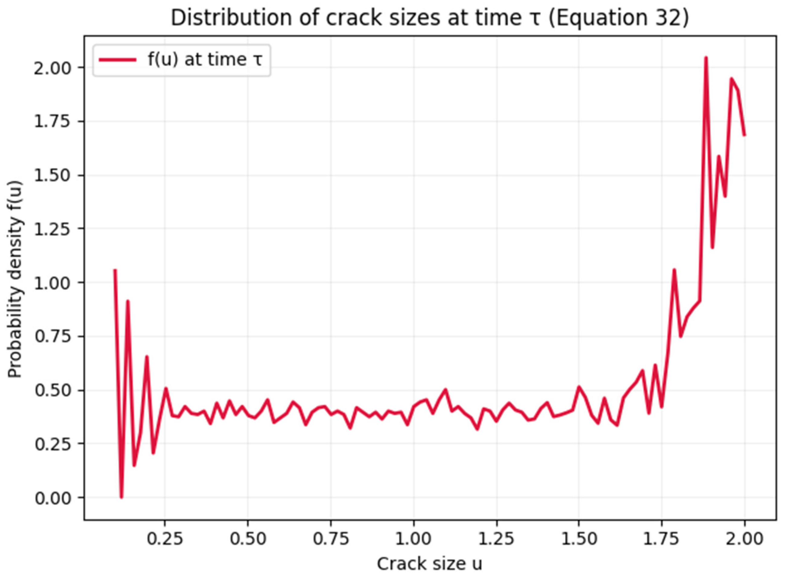
Since we are aware that it is difficult to verify the correctness of the above mathematical models, we performed the correctness check with the power of AI, namely, using ChatGPT 5. We trained ChatGPT with the entire mathematical model presented and performed a sample hypothetical case calculation. For a better understanding, AI first provided an algorithmic explanation and short code description, for example, of Equations (25)–(32), and then the corresponding calculation, the graphical representation of which is given in Figure 2. The code in this case study uses the numpy and scipy libraries for numerical calculations and matplotlib for visualization. The code is written in Python. From the results obtained, it is evident that the numerical model works logically and gives reasonable results, which will be confirmed.
Short Code Description:
  • Parameters: We define basic parameters such as the material constant (C), exponent (m), and initial crack length (a0).
  • Function for Crack Growth Rate: The crack_growth_rate( Δ   K , C, m, X) function calculates the crack growth rate based on the stress intensity factor, material constants, and the random process.
  • Random Process: The random_process(t) function simulates a random process, which can be adjusted. A normal τ distribution is used here.
  • Integration: The integrate_crack_growth(a0, C, m, Δ   K , t) function calculates the final crack length through integration.
  • Storing Results: The results of the crack length are stored in a list and displayed on a graph. Example for hypothetical non-dimensional parameters: (C = 1.0 material constant; m = 2.0 material exponent; Δ   K = np.linspace(0.1, 1.0, 100) range of stress intensity factors; a0 = 0.1 initial crack length; tmax = 10 maximum time) is presented at Figure 2.
Figure 2 confirms the results presented in Figure 13. Figure 2 shows that initially the model allows for both crack arrest and crack propagation (Figure 13a). In the middle part, we can observe the stable (slow) growth of the crack (initiation and short crack propagation), and in the final part (linear elastic growth), the spread of the crack is intense and rapid.

2.6. Intelligent Systems in Schools

The role and importance of intelligent systems have changed significantly in recent decades, especially in design and terminology. Intelligent systems have been developing intensively since the 1980s of the last century, although artificial intelligence has rarely been discussed. For the most part, however, all systems were developed primarily to support industrial applications. The names of these systems were so varied that, although they are most often known as optimization algorithms, we described our intelligent system as a knowledge-based expert system (KBES). Coding mainly used symbolic systems (classical programming languages of the time: Fortran, Basic, and C), and, less often, neural networks and similar dynamical systems (fuzzy logic and genetic algorithms), which were still in the development phase. However, systems were intensely integrated, so we obtained different hybrid systems. We used a similar philosophy in our applications, mainly because we do not have to run the whole process dynamically in education. However, there must also be specific system rules that can be strictly followed only by symbolic systems.

Knowledge-Based ESs and Other Intelligent Systems

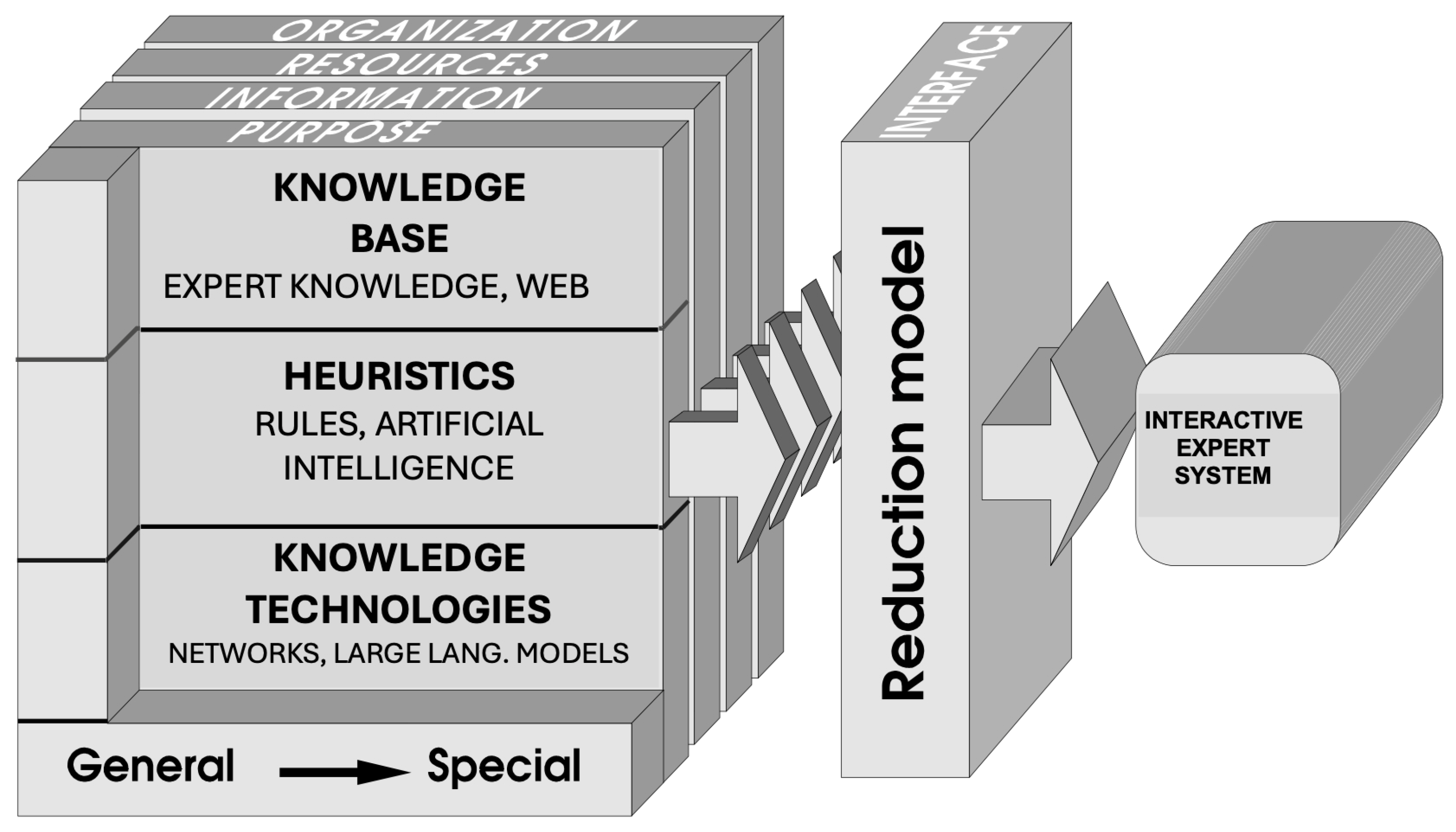
Knowledge-based expert systems (ESs) and intelligent tutoring systems are interactive computer programs providing expertise and advice on various tasks and optimization [1,2]. Aside from the main modules, the system should also seamlessly implement the following features:
  • A User Interface.
  • An Explanation Facility.
  • A Knowledge Acquisition Module, as schematically shown in Figure 3.
For example, an ES could be constructed for mechanical engineering to analyze data and simulate the design and optimization of gear transitions, as in our case. The ES could adapt its questions and tutoring style to match the student’s comprehension level.

2.7. Case Study: ITS for Gear Design

The case study presents the effectiveness of the intelligent tutoring system (ITS), particularly for modelling gear assembly that is designed for university-level (master’s and PhD) students in technical programs and programs connected with technical education. ITS (named ITS_SES) was developed and deepened for students to practice and assess their knowledge and understanding of content material and concepts in a specific manner [1,2]. The proposal led to the development of an expert system, a computer system that emulates the decision-making ability of a human expert. Expert systems were among the first truly successful forms of knowledge-based intelligence software. The intelligent tutor, supported by an expert system, is meant to train a design process for gear assembly. The result would represent optimal gearing and instructions for selecting materials, thermal treatment, mechanical manufacturing, method of lubrication, etc. The goal is to teach students to solve problems, not solve them for them. Students must show their knowledge and understanding by answering different questions during the educational process. Our ITS can adjust its questioning and tutoring according to students’ level of understanding.

2.7.1. Elements of ITS-SES

ITS-SES consists of two basic modules: (A) the module enabling a direct engineering manipulation with data, i.e., the expert system, and (B) the module providing an intelligent learning environment.
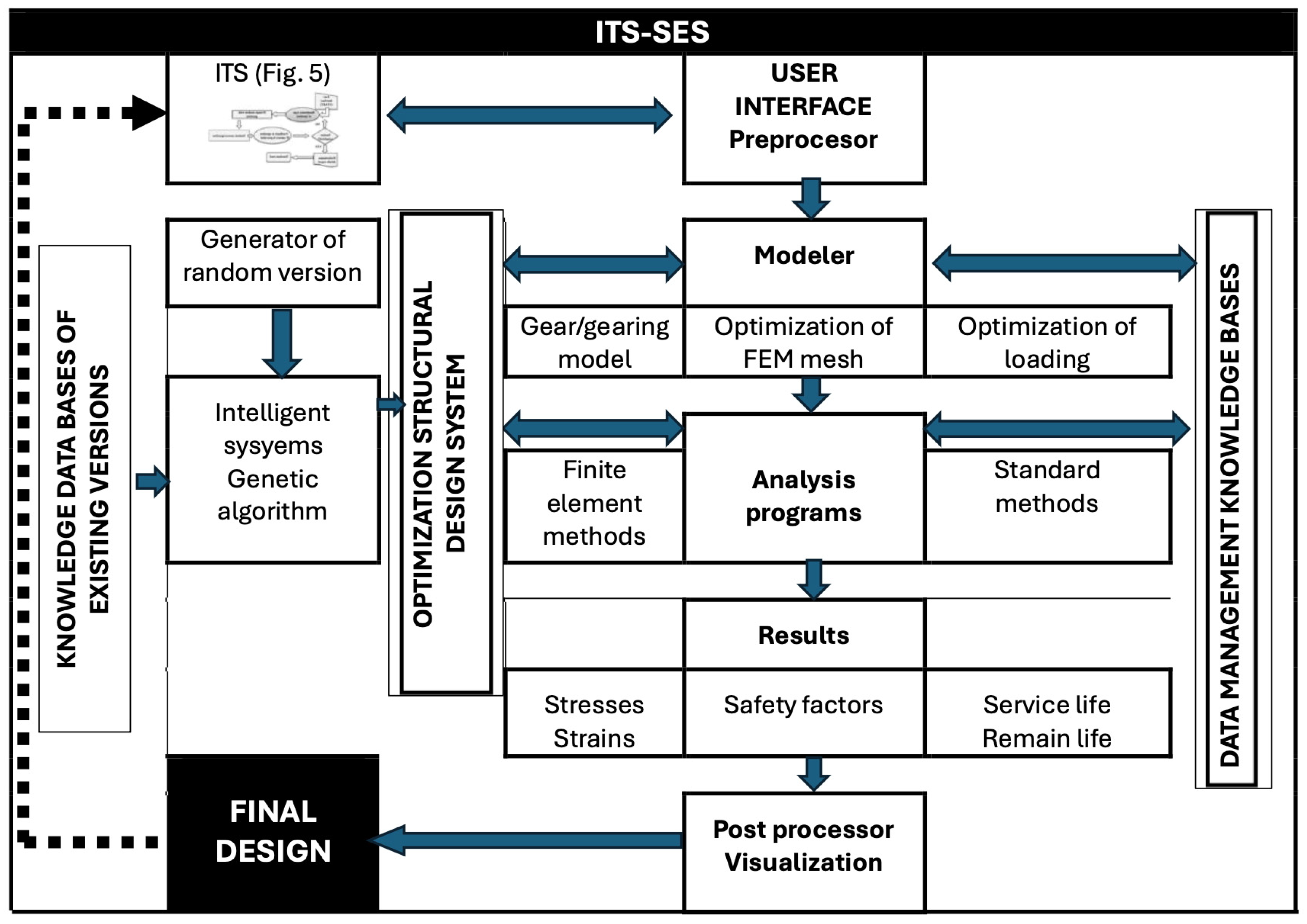
(A) Conventionally, the computer program ES consists of a pre-processor, knowledge bases, solver, and post-processor, illustrated by Figure 4.
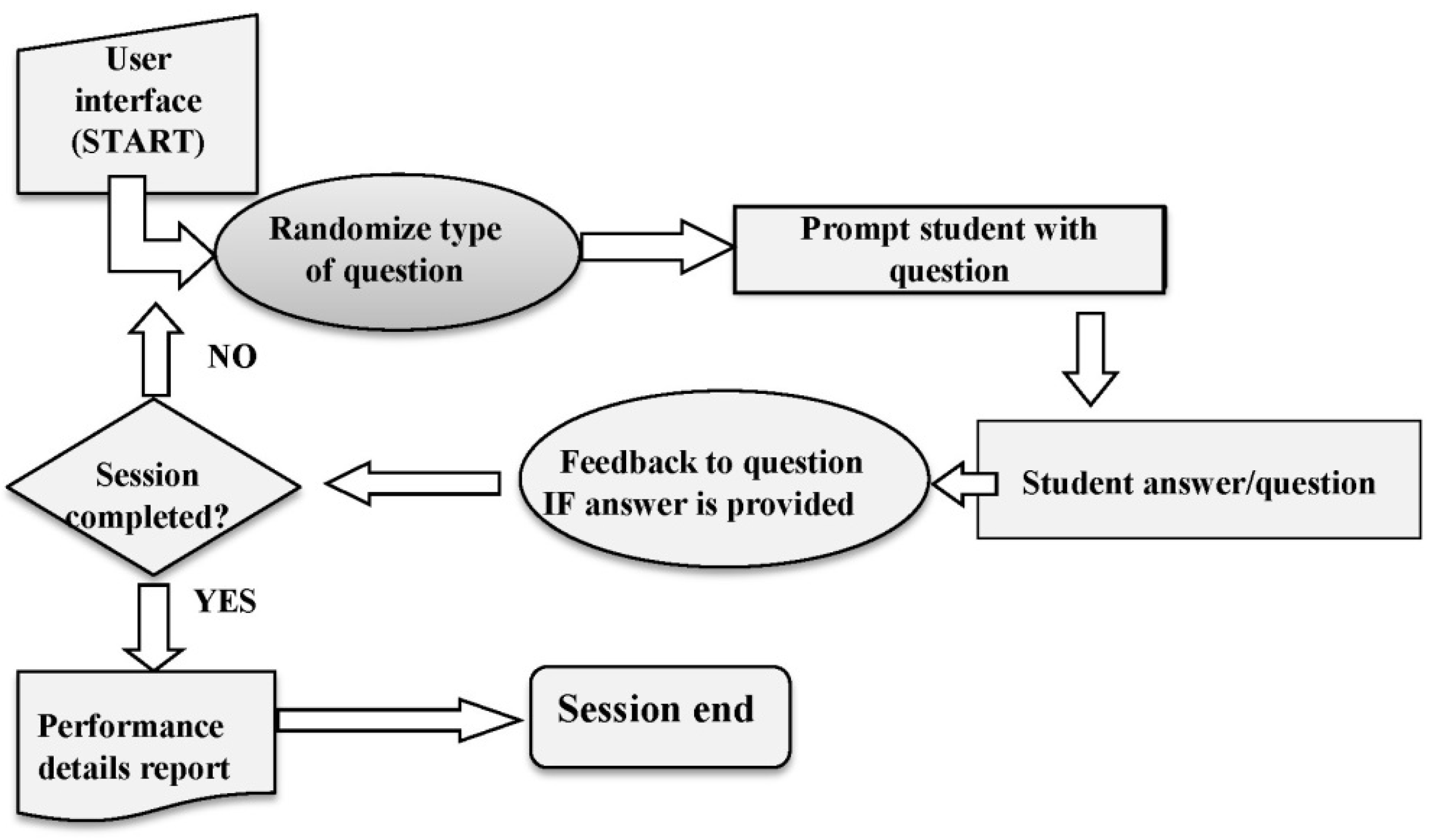
(B) The intelligent learning environment enables students and young engineers to rehearse concepts specific to a subject matter by prompting them with multiple-choice, true-or-false, and fill-in-the-blank questions, as shown in Figure 5.
Taking Intelligent tuturing ES, represented by Figure 4, and the intelligent learning environment, represented by Figure 5, we get the intelligent tutoring system ITS-SES for gear assembly design. As mentioned, ITS-SES is a hybrid cognitive system that connects two approaches to human cognition, i.e., symbol manipulations (using symbol codes) and using dynamical codes. Values put into ITS-SES based on the expert system, which is, again, intended for education on dimensioning and optimizing gear assemblies, refer to the following:
  • Geometrical values, i.e., dimensions of gears;
  • Loading (a moment of inertia and input/output moments);
  • Material characteristics;
  • Other values, such as several rotations per minute, material spring constant,
  • Stress/strain relation.
  • The pre-processor is intended for entering data, such as the following:
  • Module-m;
  • Number of teeth;
  • Centre to centre distance;
  • Coefficient of a profile displacement;
  • Inertia moments of rotating masses;
  • Spring constants;
  • Loading moments.
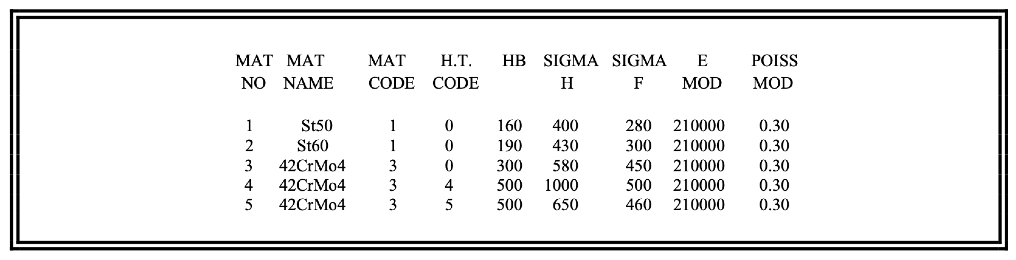
Appropriate knowledge bases are connected to the expert system, in which long-standing experience and theoretical knowledge of a field are collected. Figure 6, for example, illustrates part of a knowledge base of fundamental materials in the function of heat treatments. Descriptions of materials are given according to the DIN nomenclature: 0—structural steel, 2—case hardening steel, 3—quench and tempered steel. A number designation in the heat treatments column proceeds as follows: 0—without heat treatment, 2—case hardening, 4—flame hardening, 5—gas nitration, and 6—in-bath nitration.
MAT NO and MAT CODE is code for different materials (MAT NAME); H.T CODE is the code for heat treatment; HB is Brinell hardness (N/mm2); SIGMA H and SIGMA F is standard deviation for tensile strength ( σ ( N / m m 2 ; E is module of elasticity (dimension less), POISS MOD is Poisson module, material constant (dimension less).
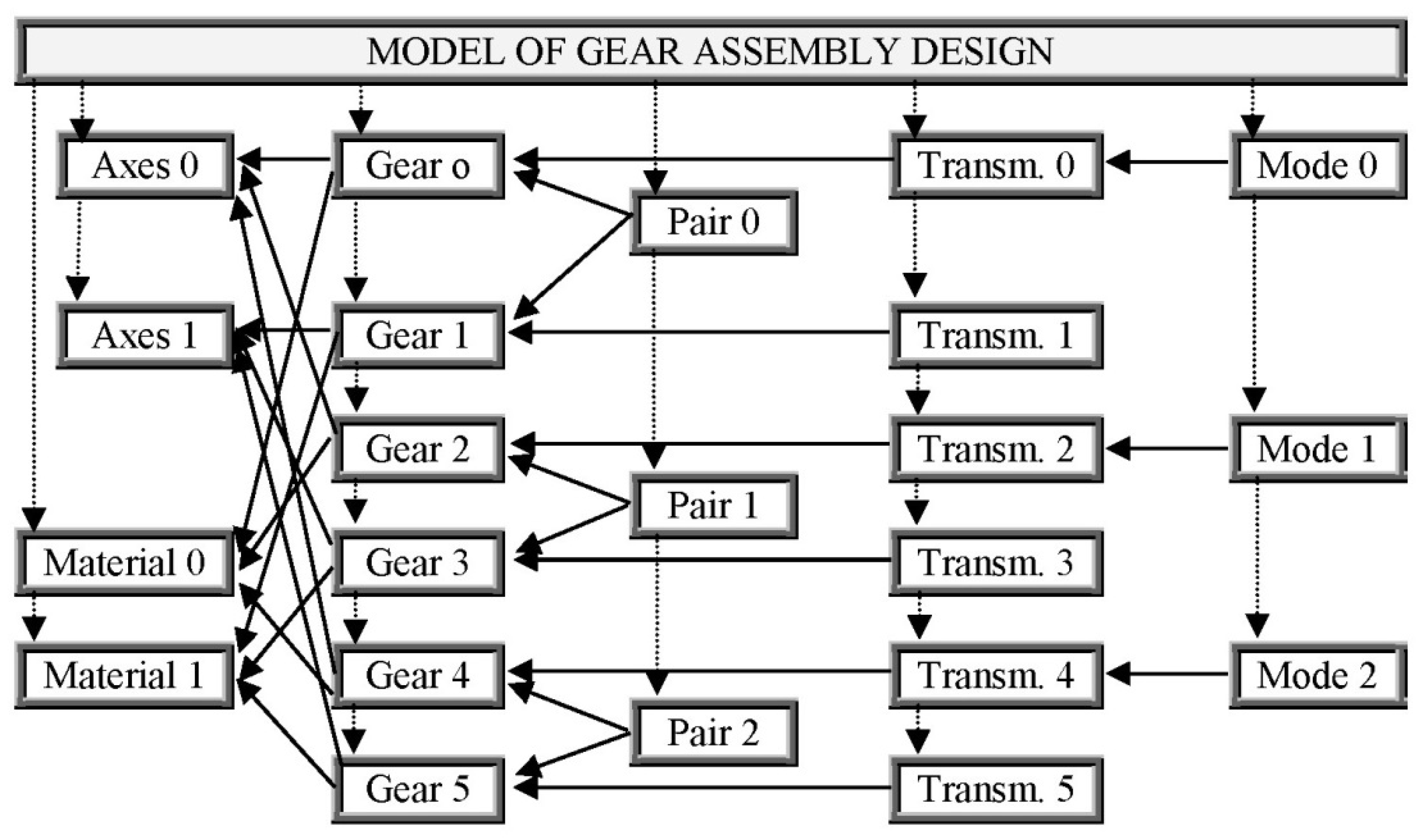
If we consider the complex structure of gear assembly, the links between basic objects are shown in Figure 7.
The Optimization Procedure Using Genetics Algorithm
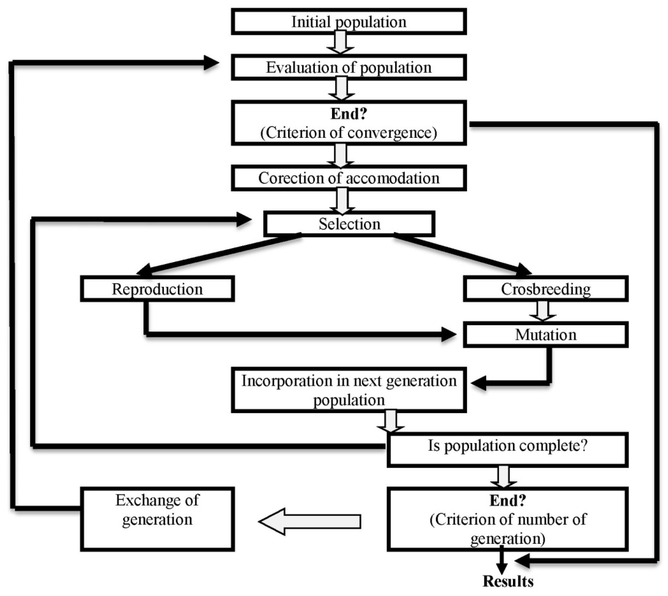
The crossover operator preserves the features (bits) that are common to both parents in the genetic algorithm, while the remaining features are mixed randomly. Figure 8 schematically illustrates the optimal algorithm, which. It was determined through numerical experimentation with various algorithms.

3. Results

3.1. Experimental Verifications

Let us just briefly reiterate the design of the entire experimental research [1,4]. Since gears and gearings belong to real, complex structures, by correctly selecting and developing test pieces and carefully planning experiments, we obtained results with which we confirmed and justified the use of the mathematical models [4] for calculating the stress intensity factor K, tooth stress intensity factor Z, as well as the service life of gears. The experimental research was carried out at the Faculty of Mechanical Engineering, University of Maribor, on the Servo-hydraulic multi-function dynamic and static test machine INSTRON 1255 ROTECH HBM-50 ROTECH.
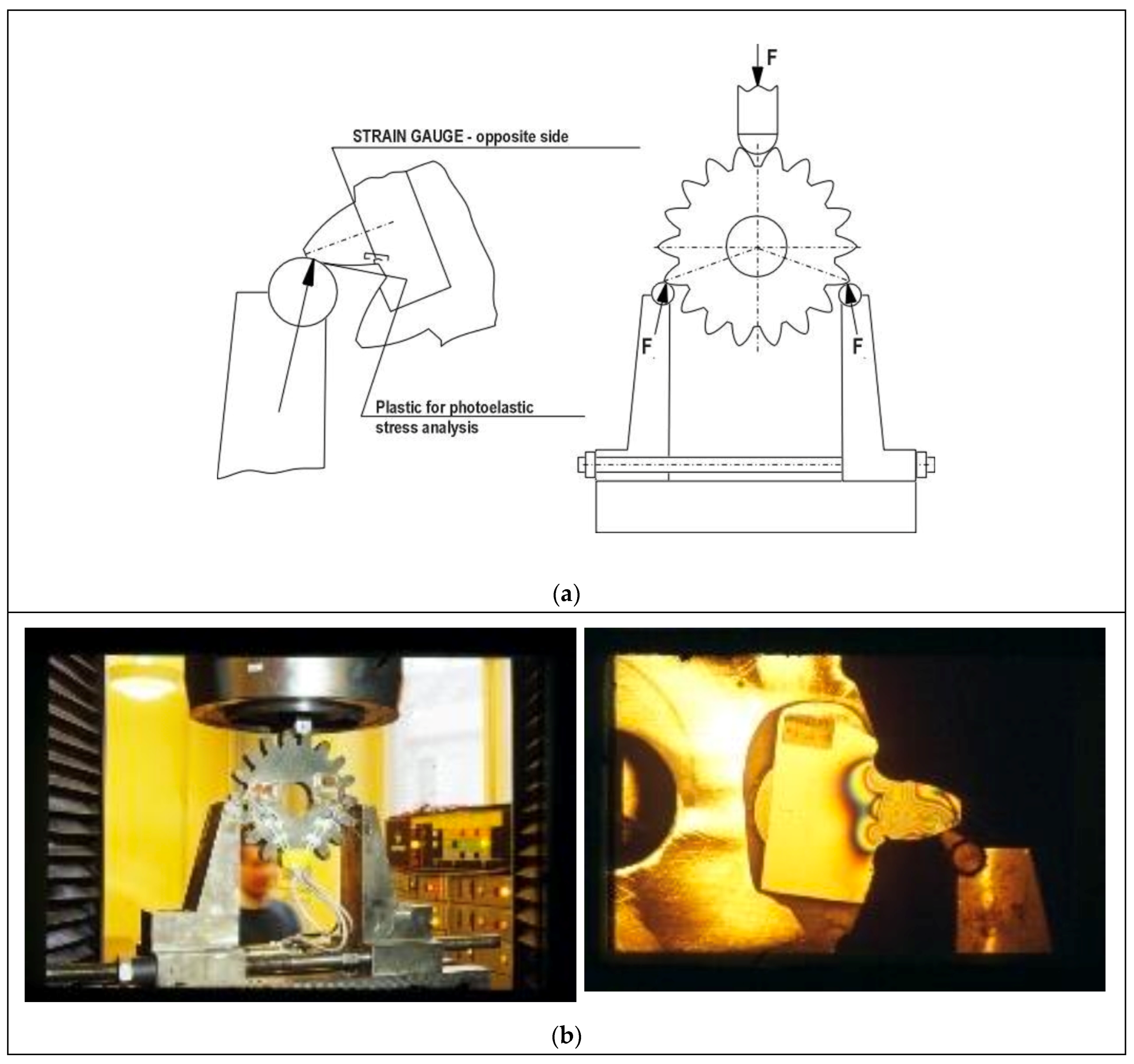
We used a non-standard test piece to determine the fracture parameters of gears. This type of test piece was a gear test piece developed during previous research [1]. A test piece together with the testing device is shown in Figure 9. We assumed that cracks would initiate in the critical cross section, i.e., the cross section with the maximum tensile stress, which proved correct based on previous research and theoretical findings. The arrangement of the individual measuring instruments is presented in Figure 9.

3.2. Measuring Method Used for Crack Initiation and Propagation

We specifically observed the initiation and propagation of short cracks. We tried to determine the conditions that would occur in this case [4] (stresses, strains, moment of beginning of fracture, etc.). For this purpose, we used mixed experimental methods: the photoelastic method, the method of measuring stress/strain using strain gauges, the replica technique for the determination of prevailing initials, and the measurement of microcracks using crack gauges. The mentioned methods were combined as follows:
  • Photoelastic examination with strain and crack gauges;
  • Strain and crack gauges;
  • Gauges with the replica method.
Combinations of different methods aimed to obtain information about the individual influences as completely as possible and determine the interaction between these magnitudes.

3.2.1. Replicas of Gears

By the replica method, we followed up the propagation of short fatigue cracks in the observed direction, i.e., along the tooth width. The test was performed to check the loadings and the ratio ΔF = Fmin/Fmax = 0.1. The test was conducted at a frequency of 50 Hz. Replicas: We made replicas in intervals of 3 × 10³ during the first three measurements, and then the step was increased to 6 × 10³ cycles. After 210 × 103, we stopped the test, and final impressions were made. All impressions were made in a critical cross-section at the point of maximum tensile stress. In the end, we created a ground section from the test piece, upon which we observed the process of crack occurrence and their size.

3.2.2. Measurements with Crack Gauges

To measure crack lengths greater than approximately 0.2 mm, we used crack gauges made by Measurement Group Vishay Type TK-09-CPB02-005. The measuring gauges were glued to gear test pieces at approximately. 0.11–0.2 mm from the edge as shown in Figure 9. Using the gauge and x-y plotter, we recorded the crack growth from the initial value to a size of 2.6 mm in ten steps. Using these measurements, we obtained the a-N curve. Based on this diagram and measurements of short crack lengths, we created the diagram da/dN—a and diagram da/dN − ΔZ.

3.3. Measuring Strain and Stress

3.3.1. Static Measurements

We loaded and unloaded the gear test piece with fixed strain gauges from stress 0 to 114 kN, and measured deformations in the critical cross-section of the gear tooth. We calculated the stress and residual stress based on deformations, i.e., especially plastic deformation in the tooth root. The results are the average value of deformations along the entire width of the strain gauge. These data were used to evaluate the results of the numerical analyses.

3.3.2. Measurements and Fatigue

During the next step, we started the fatigue test on the gear test piece at the room temperature and at 50 Hz frequency, distance between supports L = 294 mm, and ratio R = Fmax/Fmin = 0.1. During fatigue, we measured the change in strain using strain gauges as a function of the number of cycles in the area of microcracks. The basic aim of the measurements was to obtain a correlation between the micro crack length and stresses and/or to determine from the stress what happens in the material when the crack occurs. The number of cycles varied from 0 to 320,000, where the test was stopped.
The basic aim of the test was as follows:
  • To obtain a precise outline of stress fields at different points of the gear tooth, calibration of the individual methods and their comparison in the static area, in case of different stresses.
  • To find out how fatigue influences the distribution of the stress field and how it is possible, from the change in stress distribution, to assume the occurrence and growth of microcracks when non-destructive methods cannot detect them. Measurements of stresses by strain gauges and by the photoelastic method were made in intervals of 3 × 10³ for the first three measurements, and then the step was increased to 6 × 10³ cycles.
After 210 × 103, we repeated static measurements of stresses by the photoelastic method. We photographed the iso-chromates and isoclines and measured stresses using strain gauges. Thus, we obtained a precise comparison of stresses between the starting and final conditions during this test. The fundamental problem of this method is that, from the surface conditions, we assumed the interior processes. This deficiency in the gears is not excessive if the narrow gears are treated, the ratio of these being B/S < 2, i.e., where the plane stress fields can be used.

3.4. Experimental Verification of Incubation/Initiation Period

3.4.1. Crack Incubation and Initiation

As we did not have multiple different methods to choose from for the observation of what was occurring in the subjects under incubation, nor any novel methods to try out, we used only the fractographic/metallographic method to confirm the correctness of the model used and to obtain an interpretive model for describing the situation, with which we analyzed the conditions in the material. The entire experiment was carried out on three test pieces, as shown in Figure 9. The individual test piece was then loaded according to the procedure described, which was subjected to stress in the form of the following numbers of load cycles:
  • 5 × 10⁴ cycles;
  • 1 × 10⁵ cycles;
  • 2 × 10⁵ cycles.
From the experiments shown in Figure 9, we then fabricated the appropriate metallographic samples and prepared them appropriately for metallographic research on optical, quantum, and electron microscopes. In the first phase, the samples were only polished (example in Figure 10), and in the second phase, they were also subsequently etched.

3.4.2. Fractography

The fractographic research presented below was carried out in two laboratories: the laboratory for microscopic examinations at the University of Maribor, the Faculty of Mechanical Engineering, and in an industrial environment in the metallographic laboratory of the Metal Ravne factory on metallographic samples made from non-standard samples shown in Figure 10. In previous models [1,6], we determined only the consequences of the applied load, i.e., the subject’s final state, and verified the mathematical model based on this state. We found these models to exhibit good performance because they produced a reliability value between 5 and 12%. However, these models did not explain the causes and mechanisms of the phenomena that occurred in the material. In contrast, the model presented in this paper also allowed us to understand the phenomena that occurred at the nano and micro levels during the process of nucleation and crack initiation. An explanatory model serves as a helpful tool in describing and explaining why and how something functions, or why a particular phenomenon takes a certain form, which is especially important in education. It is not only important for students/young engineers to solve the problem, but they also need to understand why they have come up with the appropriate solution, and the developed model allows them to do just that. Such explanatory models do not aim to offer a complete description or explanation of the absolute reality of a phenomenon, nor do they aim to be completely accurate. However, our description/explanation aligns adequately with a significant portion of knowledge, observations, and theoretical circumstances surrounding crack incubation, which is why such an explanatory model might turn out to be very beneficial.

3.5. Confirmation Mathematical Model for the Incubation and Initiation of Cracks
Since we did not have the opportunity to trace the initiation and incubation of the crack in real time, we used the fractographic method to analyze this area. We used three test pieces, which we loaded, as in previous studies, on the Instron hydraulic pulsator. We stopped the test after 5 × 10⁴, 105, and 2 × 10⁵ cycles. We took appropriate samples from each test piece for fractographic investigations, which were carried out at the Faculty of Mechanical Engineering, University of Maribor, and at the SIJ Metal Ravne Metallographic Laboratory on optical, quantum, and row electron microscopes with magnifications of up to 180,000×. Some of the results are presented in Figure 10, Figure 11 and Figure 12.
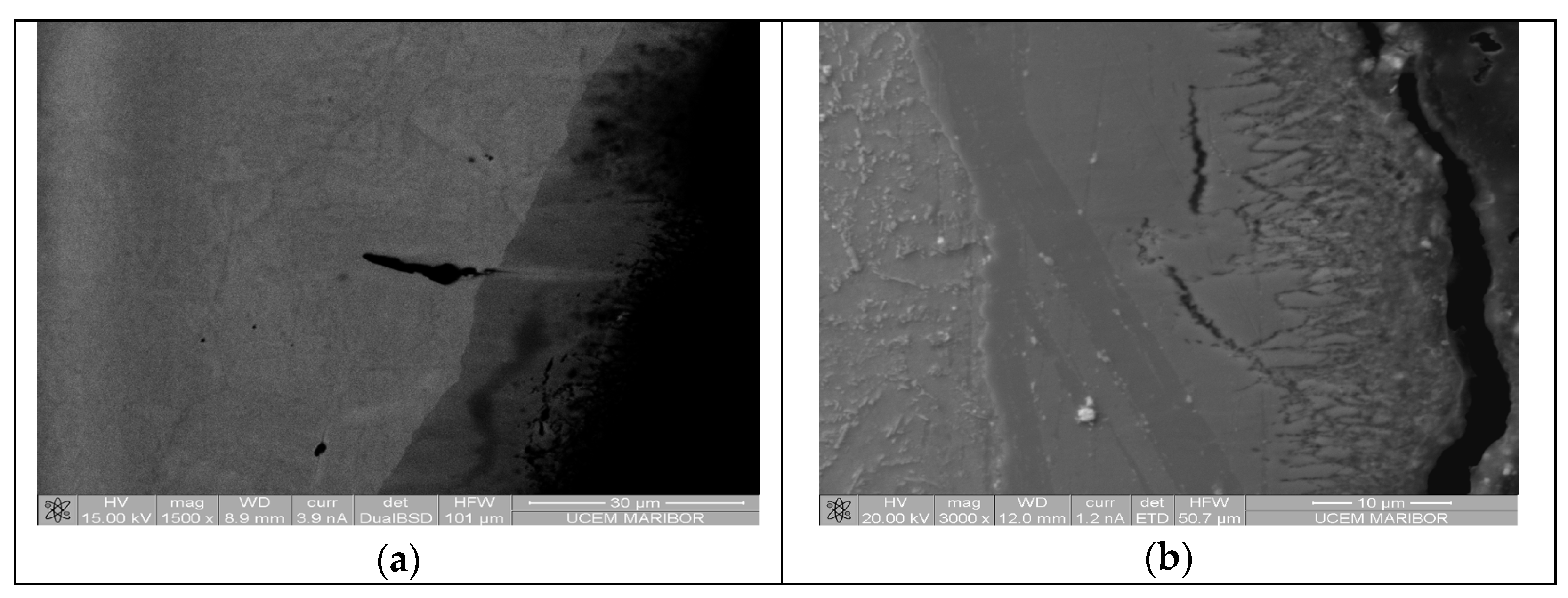
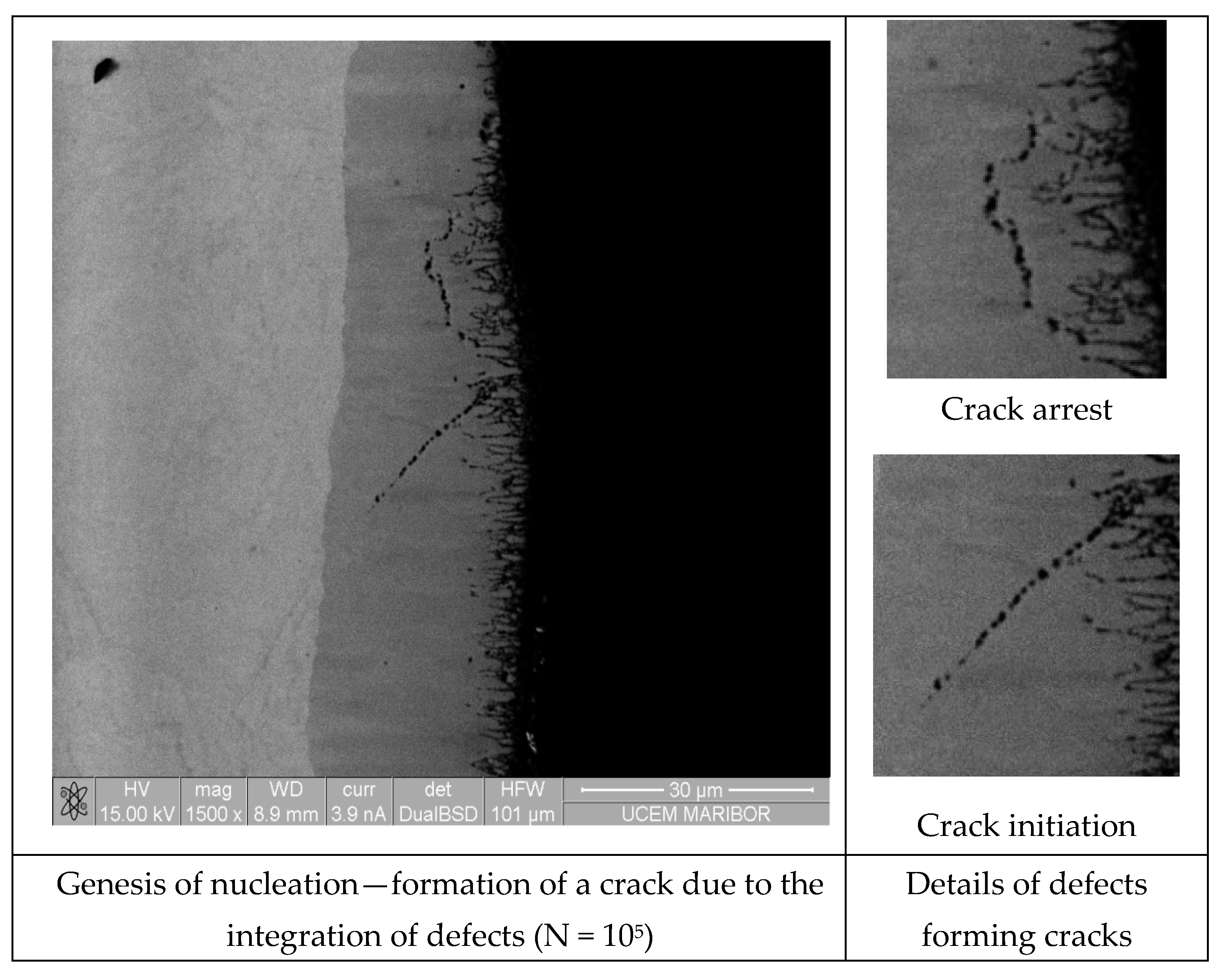
The results of the first fractographic examination after 5 × 10⁴ cycles are shown in Figure 10a, where the formation of potential initial cracking and the grouping of defects around the initial cracking and dislocations, probably in the form of micro-lunkers or similar defects, can be observed. Figure 10b presents the results of the second fractographic study after 105 load cycles, and indicates the grouping of different defects, especially in the form of dislocations, and the potential formation of initial cracking that can lead to the formation of cracks. Figure 11 thus shows two main principles underlying potential crack formation: initial cracking that does not expand (crack arrest) and can lead to pitting on gears, and initial cracking that can potentially lead to the initiation of cracks.
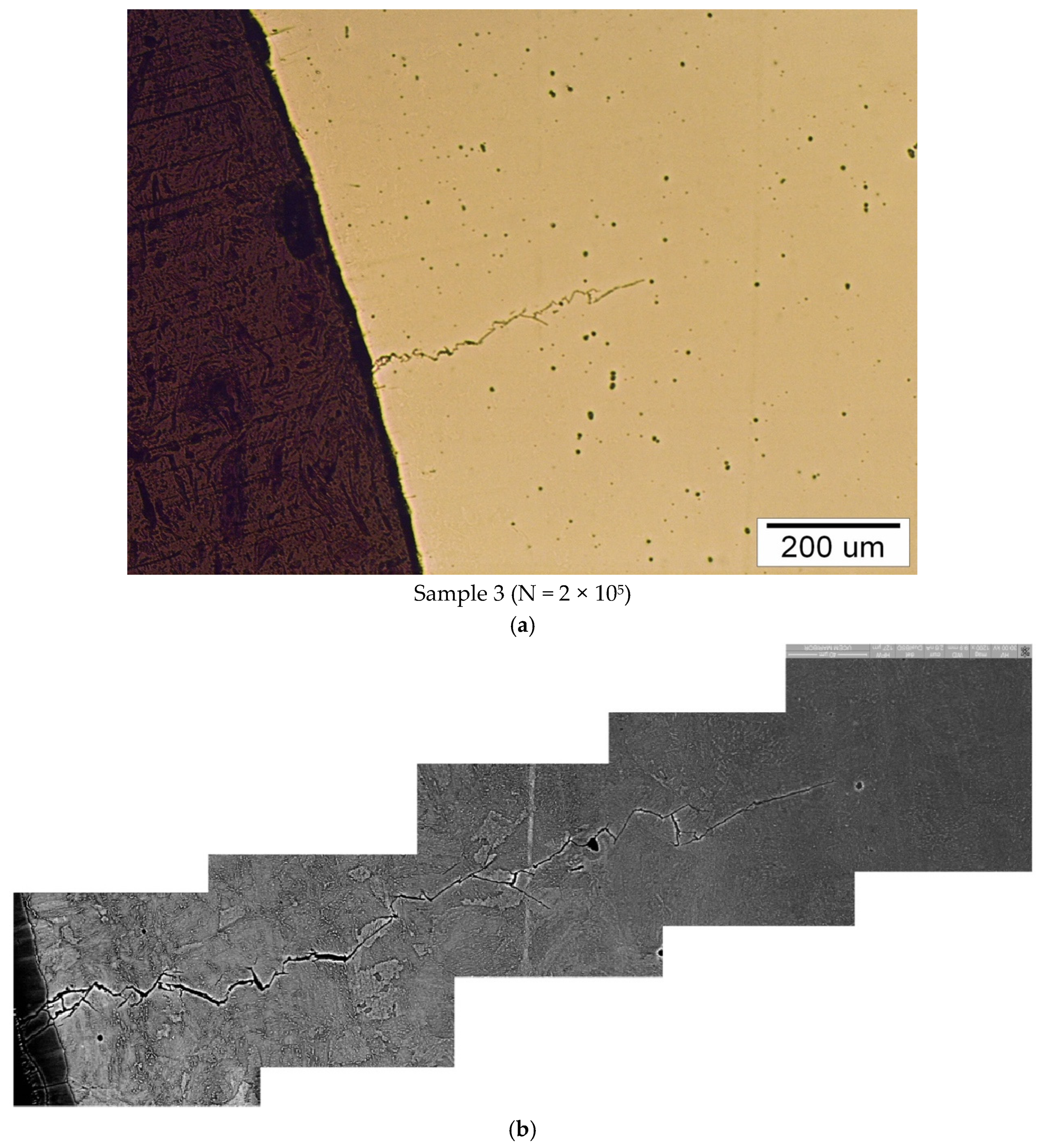
The results of the third fractographic study after 2 × 10⁵ load cycles are shown in Figure 12. Figure 12a shows the start of the spread of microstructural short cracks, from which it can be observed that the main location of crack propagation is along the boundaries of crystals. Figure 12b shows the entire course of the spread of microstructural and physical short cracks, where the crack length is at the limit of detection (approx. 500 μm), and cracks can be detected by various non-destructive detection methods that have been used in previous studies.
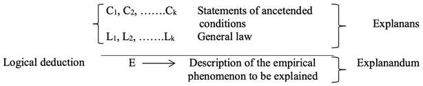
Based on this, we have developed an appropriate logical argumentation of the explanatory model, based on logical deduction and the umbrella law [16].
Futureinternet 18 00025 i001
A logical explanation should be divided into two primary components, the explanandum and the explanans, where the explanandum refers to the phenomenon to be explained (rather than the phenomenon itself), and the explanans refers to the class of sentences that are provided to explain the phenomenon. Two subclasses make up the explanans: one containing sentences (Ck—Equations (12) and (23)) with specific antecedent conditions, and the other (Lx) representing general laws (Equation (13)). For a proposed explanation to be deemed sound, its components must meet specific conditions of adequacy, which can be grouped into three logical conditions:
  • The explanandum must logically follow from the explanans;
  • The explanans must refer to general laws, and these must be genuinely necessary for deriving the explanandum;
  • The explanans must be supported by empirical content.
The explanation must also meet an empirical condition: the sentences making up the explanans must be factual (true).
It is worth noting that the same formal analysis, including the four necessary conditions, applies to both scientific prediction and explanation. The distinction between scientific prediction and explanation is of a pragmatic nature [16]. Following such logical deduction, we physically explained the values of crack incubation from 0 to 105 and divided them into the formation and cracking of defects (dislocations), with the incubation of cracks and the further grouping of defects into emerging nano cracks represented in Figure 10 and Figure 11. The further cracking of these nano/micro cracks, revealed by the fractographic studies conducted after 2 × 10⁵ cycles, can be seen in Figure 12. These results were compared with numerical and experimental results obtained in our previous research at Figure 13 [1,6].
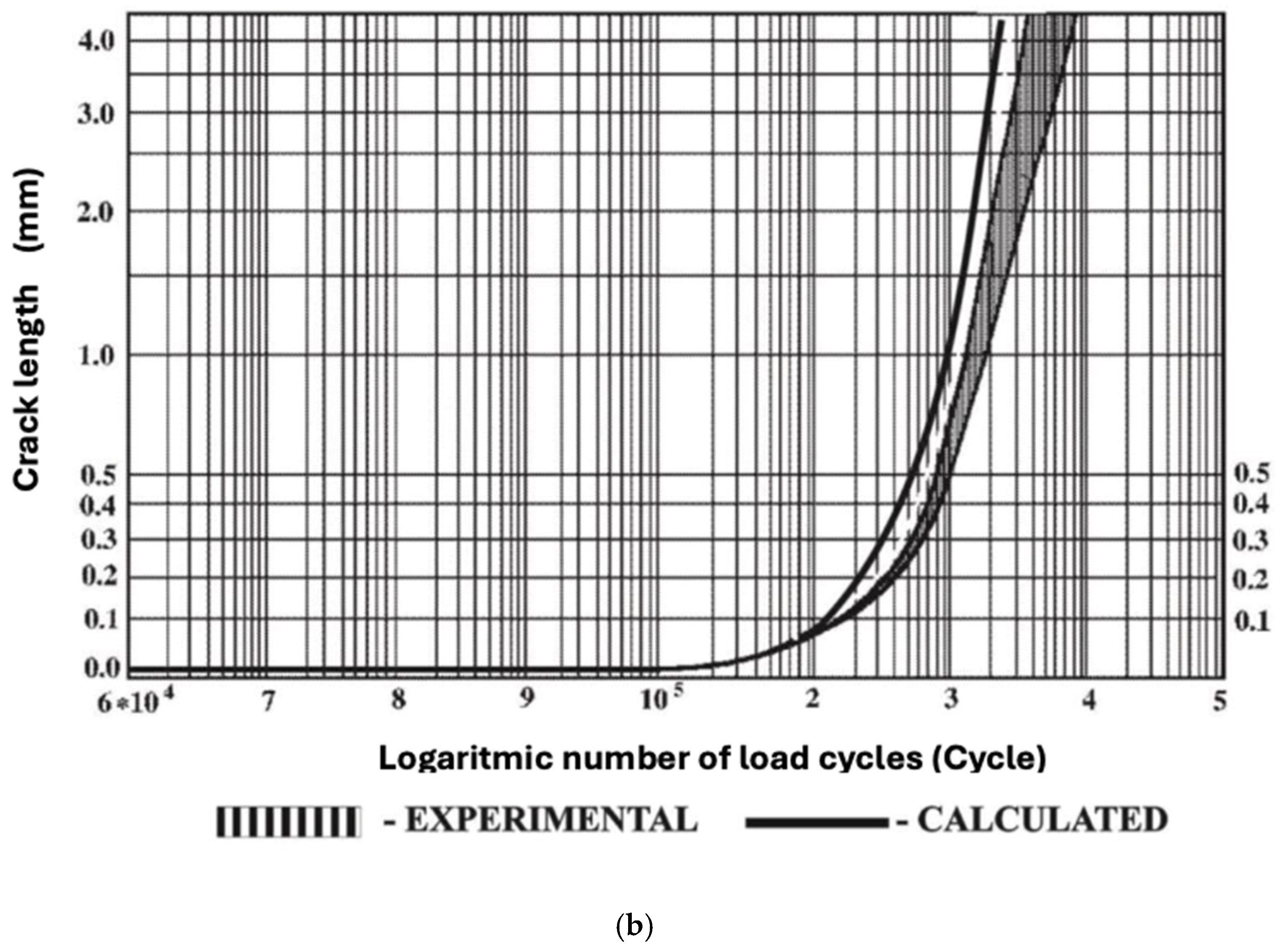
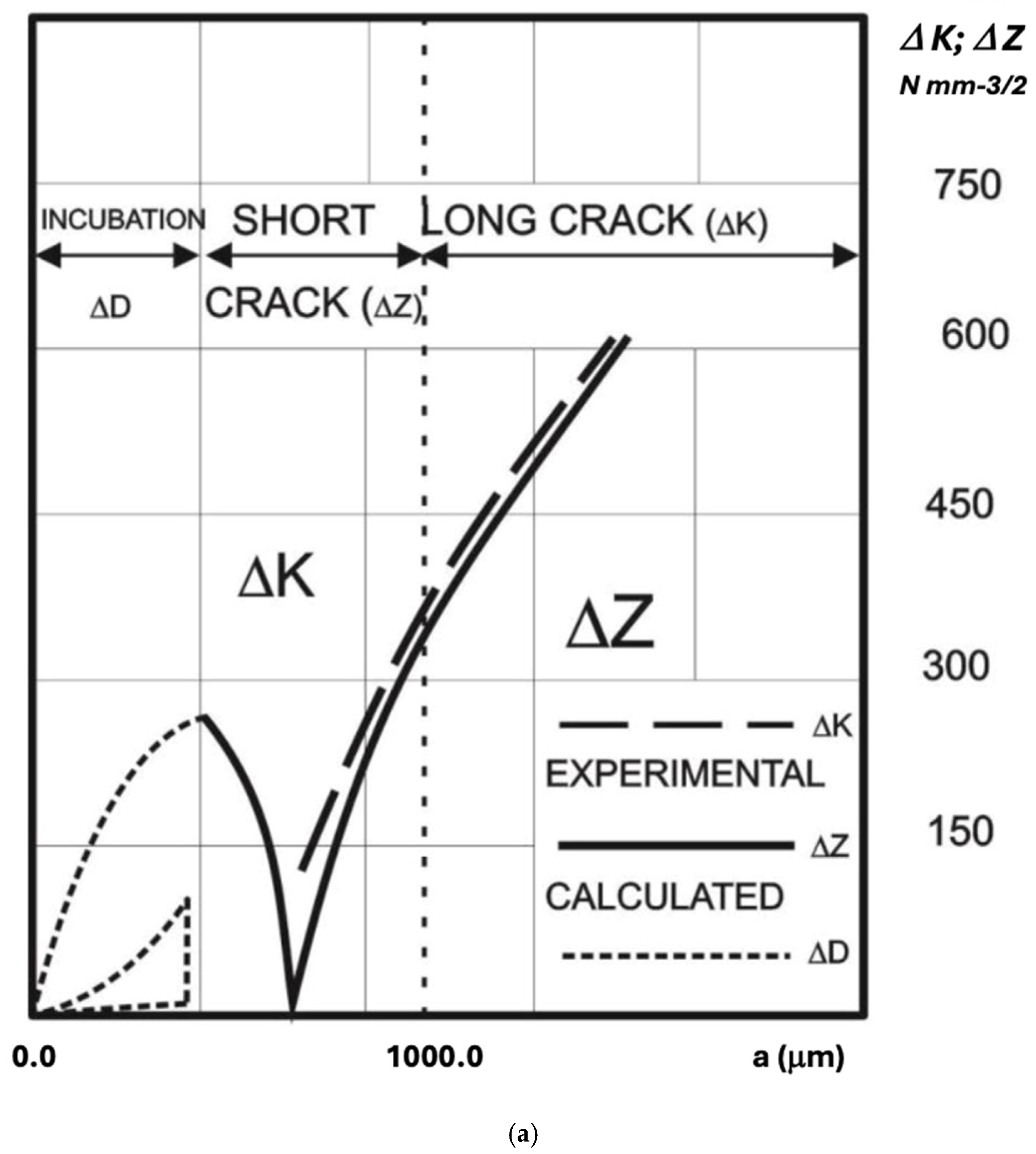
Figure 13a shows the relationship between the crack length a and the stress intensity factor ΔK or the modified tooth stress intensity factor ΔZ applicable to gears. The stress intensity factor (SIF) ΔK is considered for the general Paris law (Equation (25)) and is considered for the propagation of linearly elastic (long) cracks, for various materials, described by the material constants C and m. For the example of a gear, we have written the SIF in a modified form as a gear stress intensity factor (GSIF), which also applies to short cracks and can be calculated in a simplified way according to Equation (23). Figure 13a thus presents the relationship between the SIF or GSIF and the length of the crack a, from where we can see that the formation of the crack can be divided into three areas: incubation (a = 0–200 μm), initialization, and propagation of short cracks (a = 200–500 μm), and propagation of long linearly elastic cracks, where we can use the general SIF ΔK (which we used in the experiment) or GSIF ΔZ for crack propagation which we use in a mathematical model. Figure 13a shows that they give us very similar results.
In the presented research, special emphasis was placed on the field of incubation. For this area, we have developed a completely new mathematical model to simulate the processes that take place in the incubation of a crack. Figure 13a (and Figure 11) shows that two phenomena can occur at this stage: initials (e.g., dislocations) can merge in such a way that they do not cause the formation of a crack (Figure 11—crack arrest), or they can lead to crack generation conditions that thus pass from initials to short cracks. This area is simulated using Equations (1)–(12) with a factor of D.
In engineering applications, however, we are mainly interested in the lifetime of gears (gear transmission), which represents the ratio between the number of load cycles and the length of the crack, which is represented by Figure 13b. We can see that most of the lifetime of a gear tooth is spent in the phase of incubation and initialization of the short crack (up to a length of approx. 500 μm) and only a small part in the phase of crack propagation. Therefore, it is all the more important to have appropriate models in engineering practice to simulate the incubation and crack initialization area.

3.6. Confirmation of Mathematical Model of Crack Growth

Since we are aware that it is difficult to verify the correctness of the mathematical models used, we performed the correctness check with the power of AI, namely, using ChatGPT 5. We trained ChatGPT with the entire mathematical model presented and performed a sample hypothetical case calculation. For a better understanding, AI first provided an algorithmic explanation, and then the corresponding calculation, the graphical representation of which is given in Figure 2. The code in this case study uses the numpy and scipy libraries for numerical calculations and matplotlib for visualization. Code is written in Python. From the results obtained, it is evident that the numerical model works logically and gives good results, which are confirmed by the experimental results below.
Experimentally, we have selected a simple model for simplicity and clearness, i.e., single-step gearing with external cylindrical gears. For the required output moment Mt = 4900 Nm, gear ratio i ≅ 5, centre distance a = 315 mm, number of teeth zpinion/zgear = 21/103. We select the material AISI 4130 and nitration in a bath. The tooth width B = 80mm and coefficient of profile displacement xpinion = 0.8 and xgear = 0.258 do not change the required centre distance.
The results are shown in Figure 13, which compares the experimentally obtained data and the calculated values by applying the gear stress intensity factor Z and the proposed mathematical model. Based on the experiment and by applying standard methods, we determined the diagram ΔK-da/dN and compared it with a similar calculated diagram, i.e., ΔZ-da/dN. Based on this, we determined and calculated the service life of gears.
For example, the critical crack length was approximated at ac≅ 3.5 mm. Thus, the allowable crack ap = 1.75 mm [1,4]. The deviation increases slightly in the area approaching the material’s critical length or impact strength. Yet, perhaps most importantly, our model provided reliable results, since the final collapse of the structure in the critical area did not occur in the calculations. In practice, in deterministic calculations, we always introduce a safety factor, which ensures that the collapse of the structure is never allowed to occur (the crack reaches a critical length). Based on this, using deterministic methods based on various standards is insufficient for precise calculations of the service life of a structure. Thus, we developed a gear stress intensity factor Z (Equation (23)) for the calculations. This factor accounts not only for the stress in the critical cross-section of a homogeneous material, but also for stress concentration due to errors present within that section. Using the Z factor, we created a generalized model that, in addition to crack propagation, includes crack incubation, initiation, and growth, with the help of which the actual service life can be calculated more accurately. With the model presented here, we even achieved a slightly lower deviation compared to previous models [1,2]; we achieved a deviation of just 5 to 10% from the experimental results, which is considered highly accurate for such calculations.

3.7. ITS-SES in Education

The optimization process, included in ITS-SES, can be summed up as follows:
  • A small initial population is selected at random.
  • By using the genetic algorithm, the convergence of the population concerning a selected local criterion is effected.
  • A new population is selected, including the most successful members of the old population and new members selected randomly.
  • The procedure is stopped if the convergence criterion is met, or we return to point 2.
The primary goal when designing gear assemblies is to ensure their functionality for a certain service life. To reduce the production cost with rational use of the material, the overall dimensions of the assembly and its parts must often be optimized concerning the minimum weight. One must consider the geometric, kinematic, mechanical, tribological, technological, and economic constraints. The generalized optimization procedure consists of:
  • The definition of functionality, constraints, and selection of the optimization criteria;
  • Identification of independent variables and definition of the gear assembly model;
  • Iterative search process to find theoretically ideal gear assembly design based on a comprehensive model analysis.
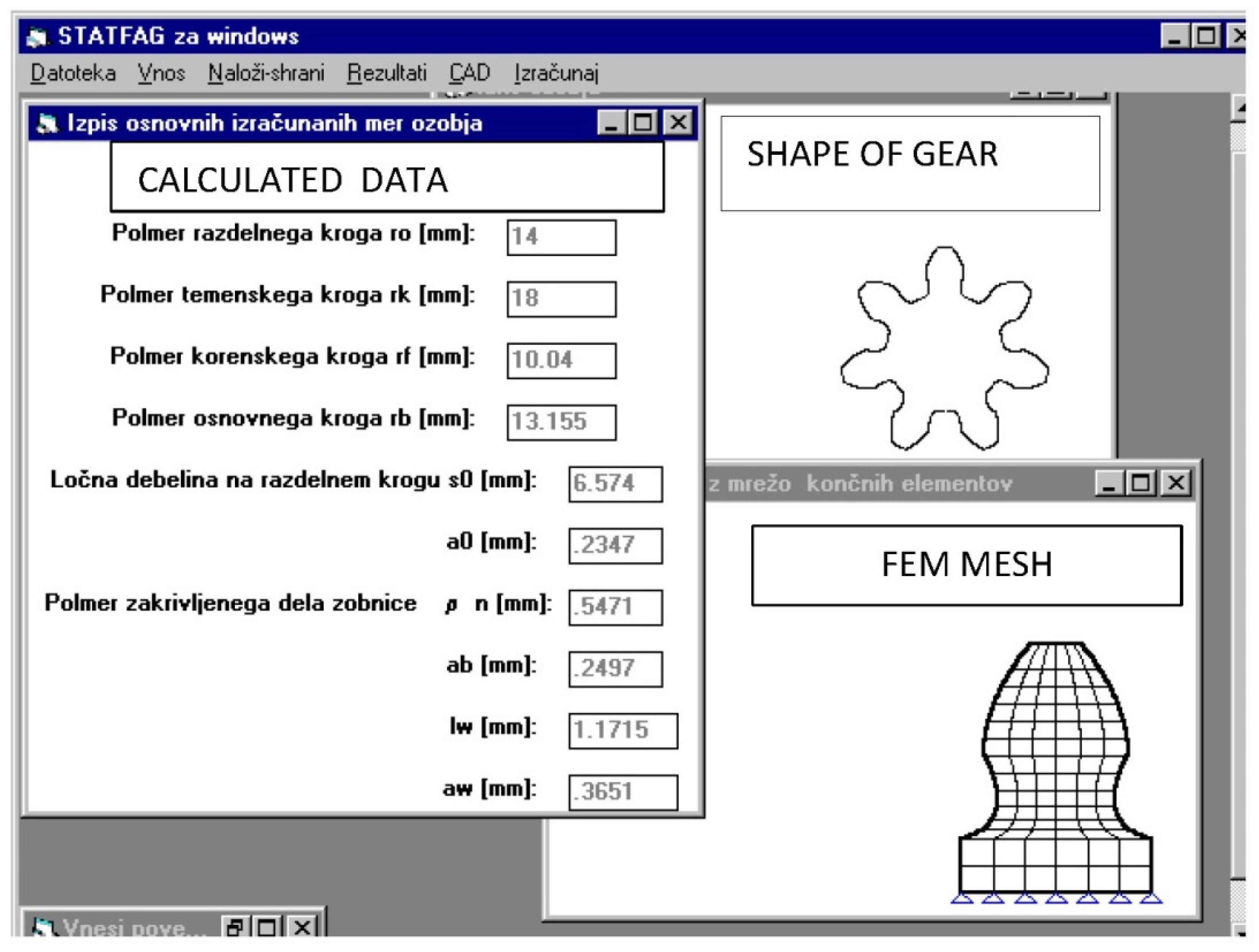
Assembly configuration, operating modes, transmitted powers, prescribed angular velocities, speed ratios, centre distances, and other prescribed features of the gear assembly have to be specified in the first step. The purpose of the optimization is to find a proper combination of gear modules, number of teeth, tooth widths, and tooth helix angles, where the objective function reaches the minimum value. The results are symbolically presented and visualized in Figure 14.
The sorts of knowledge/understanding that students absorb quickly and are, above all, the following:
  • Knowledge of the field of geometric designing: some of the results are shown in Figure 14 (the inscriptions are in Slovenian; however, they are added to show the basic principle of the operation), and from them it is evident, for example, how the number of teeth influences the shape of them, how the undercut of a gear root begins, how can appropriate profile movements, etc., prevent this;
  • Knowledge of the field of strength calculations: connections between the shape and stresses in a tooth root, connections among a material, shape, and service life;
  • Knowledge about heat treatment selected from the knowledge base form (see Figure 6),

4. Discussion

For the determination of crack incubation and initialization, we incorporated our developed code (Equations (1)–(12)) into a model used in previous research [1,2]. Through this, we were able to combine both studies and use the findings of this previous research to determine and explain the entire lifespan of a crack and explain the phenomena of incubation and crack initiation, in our case, for a crack in the root of a gear tooth.
To confirm our model’s accuracy in calculating service life, we carried out two types of investigations: one related to the initiation and incubation of cracks, in an area where no appropriate experimental methods were available for tracing the strain/stress state in real time; and the other related to the crack propagation from an area of micro to macro size, for which purpose, contrastingly, there are a number of experimental methods available.
Let us devote a little more space to the explanation of crack incubation and initiation, since the crack propagation model has been described in our previous research [1,2], and we have only briefly repeated and summarized the explanations here. The results shown in Figure 9 and Figure 13 show a comparison between the data obtained experimentally and the values calculated using the suggested mathematical models. Based on experiments and using standard methods (general law, Equations (13) and (25)), we established a diagram ΔKa and compared it to a similarly calculated diagram, i.e., ΔZ/Da (explanandum, Equations (12) and (23)). Based on this, we calculated the gears’ service life to be approximately 3.3 × 10⁵ load cycles. If we compare this with the experimental data of 3.5–3.8 × 10⁵, we can conclude that the deviation is more acceptable. However, it is also important that when using our proposed model, the resulting calculation always stays on the safe side. We have created a model that not only provided us with good results, but also explained the mechanisms occurring in an area where it was almost impossible to determine the conditions of incubation and early crack initiation. In the classical, deterministic approach, we can say that we have achieved a safety factor of 1.05–1.12, which is an extremely low safety factor for dynamical systems in standardized calculations (it is usually greater than 2). Since we have developed an explanatory model for the incubation of cracks, this model also gives us a deeper insight into developments that we have not been able to follow so far, which is also extremely important in the education process in the engineering professions. For this reason, we have prepared a learning environment intended not only to be used in the optimization process, but also to be important in understanding the physical background. That is why we have also adapted an appropriate intelligent tutoring system, ITS-SES, for the learning process, where we have combined many years of research and the experience gained in this way with modern educational trends.
The role and importance of intelligent systems have changed significantly in recent decades, especially in design and terminology. Intelligent systems have been developing intensively since the 1980s of the last century, although artificial intelligence has rarely been discussed. For the most part, however, all systems were developed primarily to support industrial applications. The names were so varied that, while such systems are most often described as optimization algorithms, we described our intelligent system as a knowledge-based expert system (KBES). Coding was mainly performed using symbolic systems (classical programming languages of the time, Fortran, Basic, and C), and less often neural networks and similar systems (fuzzy logic and genetic algorithms), which were still in development.
Nevertheless, there has been some interweaving of the two programming systems, in various forms of hybrid systems that have been complemented by hybrid forms of teaching [17,18], most often blended learning [19,20]. We have also joined these modern trends in learning and teaching with intelligent tutoring systems [21,22]. One of these is also presented in this article.

5. Conclusions

Education is transforming significantly from the traditional approach, which places students in a passive learning position. Today’s progressive learning environment is seeing the popularity of outcome-based teaching methods based on non-formal distance learning, teamwork, and KBES (AI). The effectiveness of these changes indicates the need for a large-scale reconceptualization and transformation of the learning process. Achieving this will require teachers to engage students as independent and active learners. Powerful new technologies are needed to establish an information-rich and intelligent learning environment where students and teachers can navigate various informational superhighways. One such option is presented in this paper.
Importantly, we have not only provided students with an optimization model for the construction of gears, but also an explanatory model that explains what is happening in an area where it is almost impossible to determine the conditions of incubation and early initialisation of cracks. This model will give students the knowledge and critical thinking to develop and optimize appropriate solutions. Of course, there is still much to be done at the presented ITS-SES. That is why we are researching the system of learning environments in two directions. In the pedagogical field, we are developing appropriate generative pedagogy that treats AI (KBES) as a partner in teaching and not just as a tool. At the same time, in the technological field, we are developing sharp learning partners, intelligent agents who can take on the role of an active participant in the learning process in ITS-SES. Of course, technological developments in this area are so rapid that we can no longer adequately keep up with the progress of technology in education.

Author Contributions

Conceptualization, B.A. and S.K.; methodology, A.F.; calculation and mathematical model: Section 2.2 and Section 2.3, S.K.; Section 2.4 and Section 2.5, B.A.; Section 2.6 and Section 3.7, A.F.; Experiment B.A.; formal analysis, S.K. and B.A.; writing—original draft preparation, B.A.; writing—review and editing, S.K. and A.F. All authors have read and agreed to the published version of the manuscript.

Funding

This research received no external funding.

Data Availability Statement

The original contributions presented in this study are included in the article. Further inquiries can be directed to the corresponding authors.

Conflicts of Interest

The authors declare no conflicts of interest.

References

  1. Aberšek, B.; Flašker, J. How Gears Break; WIT Press: Southampton, UK, 2004. [Google Scholar]
  2. Aberšek, B.; Flašker, J.; Glodež, S. Review of mathematical and experimental models for determination of service life of gears. Eng. Fract. Mech. 2004, 71, 439–453. [Google Scholar] [CrossRef] [Scilit]
  3. Buehler, M.J.; Dodson, J.; van Duin, A.C.T.; Meulbroek, P.; Goddard, W.A., III. The Computational materials Design Facility (CMDF): A powerful framework for multiparadigm multi-scale simulations. Mater. Res. Soc. Proc. 2006, 894, LL3.8. [Google Scholar] [CrossRef] [Scilit]
  4. Aberšek, B.; Flašker, J. Experimental Analysis of Propagation of Fatigue Crack on Gears. Exp. Mech. 1998, 38, 226–230. [Google Scholar] [CrossRef] [Scilit]
  5. Provan, J.W. Probabilistic Fracture Mechanics and Reliability; Martinus Nijhoff Publishers: Dordrecht, The Netherlands; Boston, MA, USA; Lancaster, UK, 1987. [Google Scholar]
  6. Spergel, D.N.; Turok, N.G. Textures and cosmic structure. Sci. Am. 1996, 266, 52–59. [Google Scholar] [CrossRef] [Scilit]
  7. Zurek, W.H. Cosmological experiments in condensed matter. Phys. Rep. 1984, 276, 177–221. [Google Scholar] [CrossRef] [Scilit]
  8. Imry, Y.; Ma, S. Random-Field Instability of the Ordered State of Continuous Symmetry. Phys. Rev. Lett. 1975, 35, 1399–1402. [Google Scholar] [CrossRef] [Scilit]
  9. Aharony, A.; Pytte, E. Infinite Susceptibility Phase in Random Uniaxial Anisotropy Magnets. Phys. Rev. Lett. 1980, 45, 1583–1587. [Google Scholar] [CrossRef]
  10. Bellini, T.; Buscaglia, M.; Chiccoli, C.; Mantegazza, F.; Pasini, P.; Zannoni, C. Nematics with quenched disorder: What is left when long range is disrupted? Phys. Rev. Lett. 2000, 31, 1008–1011. [Google Scholar] [CrossRef] [Scilit] [PubMed]
  11. Mermin, N.D. The topological theory of defects in ordered media. Rev. Mod. Phys. 1976, 51, 591–648. [Google Scholar] [CrossRef] [Scilit]
  12. Lubensky, T.C.; Renn, S.R. Twist-grain-boundary phases near the nematic–smectic-A–smectic-C point in liquid crystals. Phys. Rev. A 1990, 41, 4392–4401. [Google Scholar] [CrossRef] [Scilit]
  13. Abrikosov, A.A. On the Magnetic Properties of Superconductors of the Second Group. Sov. Phys. JETP 1957, 5, 1174–1182. [Google Scholar]
  14. De Gennes, P.G.; Prost, J. The Physics of Liquid Crystals; Oxford University Press: Oxford, UK, 1993. [Google Scholar]
  15. Taylor, D.; Knott, J.F. Fatigue crack propagation behaviour of short crack; the effect of microstructure. Fatigue Engn. Mater. Struct. 1981, 4, 147–155. [Google Scholar] [CrossRef] [Scilit]
  16. Hempel, C.G. Aspects of Scientific Explanation and Other Essays in the Philosophy of Science; The Free Press: New York, NY, USA, 1965. [Google Scholar]
  17. Li, K.C.; Wong, B.T.M.; Kwan, R.; Chan, H.T.; Wu, M.M.F.; Cheung, S.K.S. Evaluation of Hybrid Learning and Teaching Practices: The Perspective of Academics. Sustainability 2023, 15, 6780. [Google Scholar] [CrossRef] [Scilit]
  18. Almufarreh, A.; Arshad, M. Promising Emerging Technologies for Teaching and Learning: Recent Developments and Future Challenges. Sustainability 2023, 15, 6917. [Google Scholar] [CrossRef] [Scilit]
  19. Gligorea, I.; Cioca, M.; Oancea, R.; Gorski, A.-T.; Gorski, H.; Tudorache, P. Adaptive Learning Using Artificial Intelligence in e-Learning: A Literature Review. Educ. Sci. 2023, 13, 1216. [Google Scholar] [CrossRef] [Scilit]
  20. Gamage, K.A.A.; Gamage, A.; Dehideniya, S.C.P. Online and Hybrid Teaching and Learning: Enhance Effective Student Engagement and Experience. Educ. Sci. 2022, 12, 651. [Google Scholar] [CrossRef] [Scilit]
  21. Wypych, G. Atlas of Material Damage; ChemTec Publishing: Toronto, ON, USA, 2022. [Google Scholar]
  22. Lin, C.C.; Huang, A.Y.Q.; Lu, O.H.T. Artificial intelligence in intelligent tutoring systems toward sustainable education: A systematic review. Smart Learn. Environ. 2023, 10, 41. [Google Scholar] [CrossRef] [Scilit]
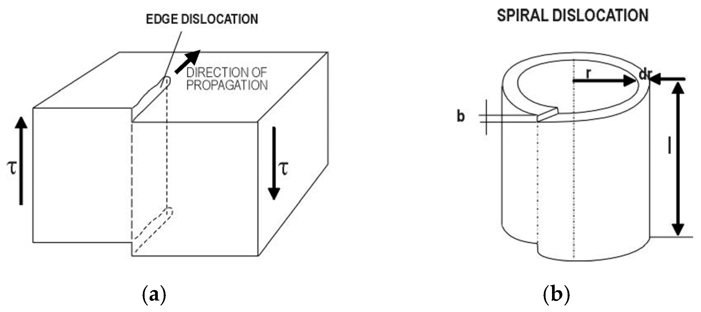
Figure 1. Edge dislocation (a) and spiral dislocation (b).
Futureinternet 18 00025 g001
Figure 2. Distribution of the crack length according to time τ corresponding to probability density function fu.
Futureinternet 18 00025 g002
Figure 3. The configuration of our expert system [1].
Futureinternet 18 00025 g003
Figure 4. ITS-SES intelligent tutoring system.
Futureinternet 18 00025 g004
Figure 5. Flow Chart of QUESTION-ANSWER process between students and intelligent learning environment.
Futureinternet 18 00025 g005
Figure 6. Knowledge base of basic materials and heat treatments.
Futureinternet 18 00025 g006
Figure 7. Links between basic objects of gear assembly.
Futureinternet 18 00025 g007
Figure 8. Flowchart of optimization procedure.
Futureinternet 18 00025 g008
Figure 9. Testing device with test piece (a) and different stress/strain measurement techniques (b).
Futureinternet 18 00025 g009
Figure 10. (a) Sample 1 after the 5 × 10⁴ load and (b) Sample 2 after the 105 load.
Futureinternet 18 00025 g010
Figure 11. Sample 2 after the 105 load.
Futureinternet 18 00025 g011
Figure 12. (a) Sample on scale 200 μm after approx. N = 2 × 10⁵; (b) Genesis and growth of microcracks (approx. 500 μm long after approx. N = 2 × 10⁵).
Futureinternet 18 00025 g012
Figure 13. (a) Initiation and crack propagation; (b) lifetime curves for gear tooth [1,6].
Futureinternet 18 00025 g013aFutureinternet 18 00025 g013b
Figure 14. Results produced by post-processor.
Futureinternet 18 00025 g014
Disclaimer/Publisher’s Note: The statements, opinions and data contained in all publications are solely those of the individual author(s) and contributor(s) and not of MDPI and/or the editor(s). MDPI and/or the editor(s) disclaim responsibility for any injury to people or property resulting from any ideas, methods, instructions or products referred to in the content.