

Lightweight Anomaly Detection in Digit Recognition Using Federated Learning


Abstract
1. Introduction
- We design, implement, and evaluate several fully connected autoencoder models for digit-based anomaly detection, deployed fully on the ESP32-CAM microcontroller. Our approach enables on-device training and inference using standard 32-bit floating-point precision and incorporates an innovative dual-phase early stopping mechanism to optimize training efficiency. The best-performing models achieve an F1 score of up to 0.87 when optimized for MNIST and EMNIST anomaly detection, with on-device training times as short as 12 min and inference latency as low as 9 ms.
- We implement a real-world federated learning testbed across 10 ESP32-CAM devices and test various IID and non-IID data distributions, including corrupted datasets, to reflect realistic edge scenarios. Our extensive experimental results demonstrate strong and consistent F1 scores, achieving up to 0.87 in the standard IID setting and 0.86 in the extreme non-IID setting.
- We analyze the robustness and resilience of FL in the presence of heterogeneous and corrupted data sources without relying on explicit malicious device detection. We evaluate scenarios where one to five out of the ten devices have corrupted datasets. The results show that federated aggregation effectively mitigates the impact of anomalous datasets, rendering their influence negligible for up to two corrupted devices and causing only minor performance degradation when more devices are affected.
- We characterize the ESP32-CAM’s memory footprint by analyzing program size, dataset allocation, and memory consumption during training and inference to establish practical limits for embedded model deployment. The results demonstrate that more than half of the evaluated models fit entirely within the internal RAM, enabling faster training speeds while maintaining satisfactory performance.
2. Related Work
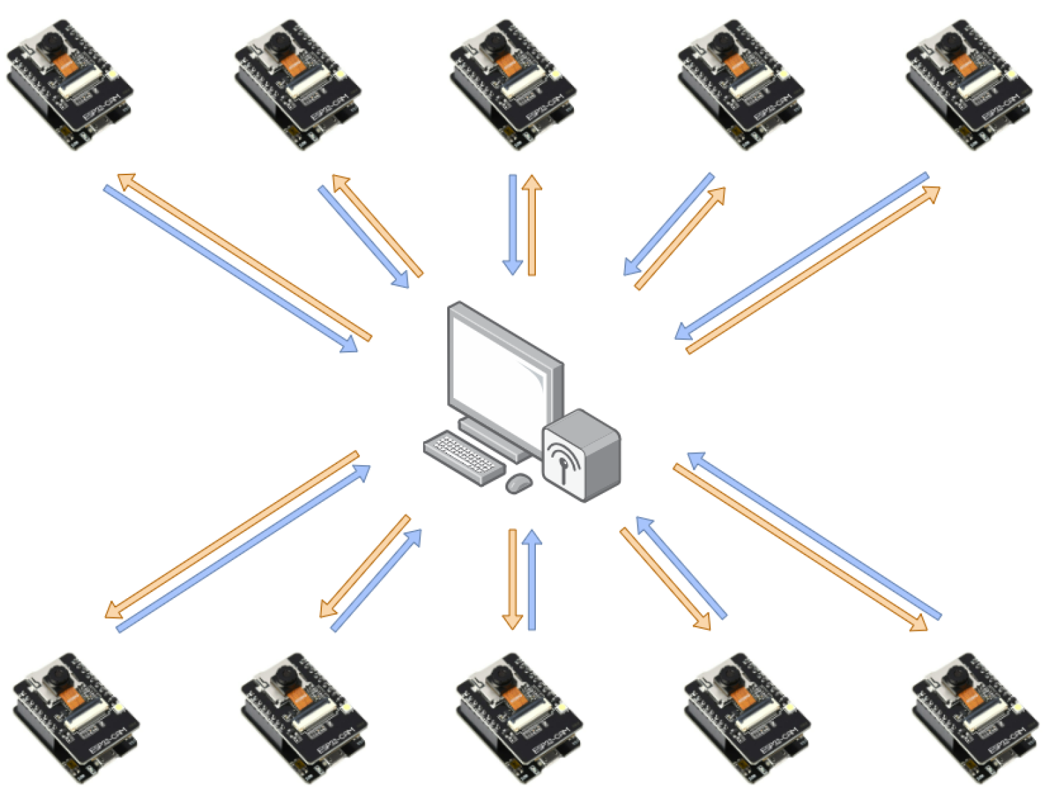
3. System Architecture
- Data collection: Capture sensor or image data.
- On-device training: Train lightweight ML models locally.
- Federated participation: Exchange model parameters with the server during the FL.
- Training configuration: Sending configuration parameters to devices, such as the number of epochs, learning rate, and model structure.
- Model aggregation: Receiving local model updates from devices, aggregating them into a global model, and distributing the updated model.
- Model synchronization: Providing the latest global model to devices that rejoin the training process after disconnection or power loss.
4. Autoencoder Deployment on ESP32-CAM
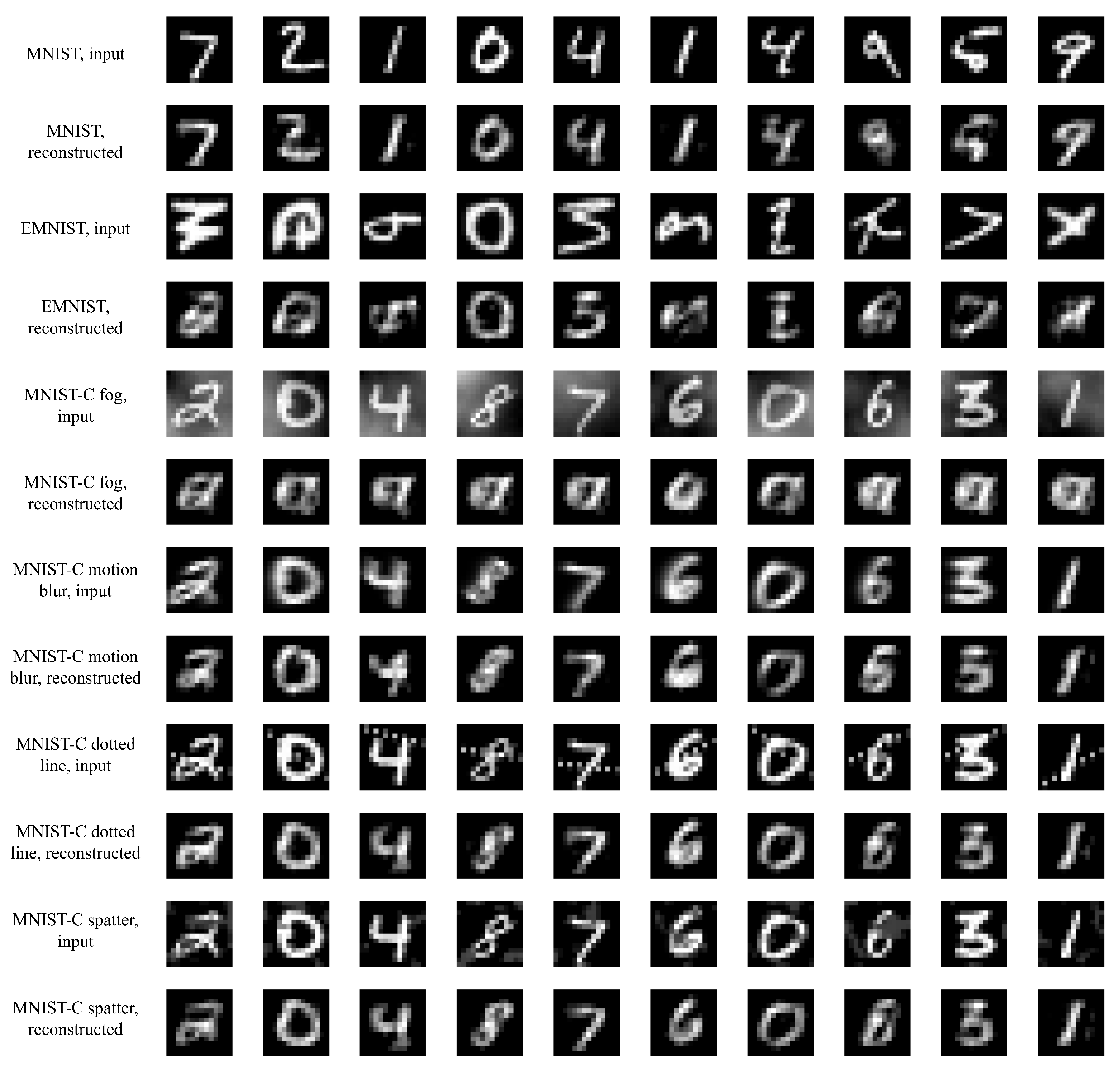
4.1. Dataset Selection and Modification
4.2. Model Architecture and Training Strategy
- Model 1: Single hidden layer with 16 neurons—architecture: [196, 16, 196].
- Model 2: Single hidden layer with 32 neurons—architecture: [196, 32, 196].
- Model 3: Single hidden layer with 64 neurons—architecture: [196, 64, 196].
- Model 4: Two hidden layers with 32 neurons each—architecture: [196, 32, 32, 196].
- Model 5: Three hidden layers with a narrow bottleneck of 8 neurons—architecture: [196, 32, 8, 32, 196].
- Model 6: Three hidden layers with a narrow bottleneck of 16 neurons—architecture: [196, 64, 16, 64, 196].
- Model 7: Five hidden layers with 32-neuron bottlenecks and wider 64-neuron outer layers—architecture: [196, 64, 32, 32, 64, 196].
4.3. Embedded Deployment and Training
5. Federated Training of Edge Autoencoders
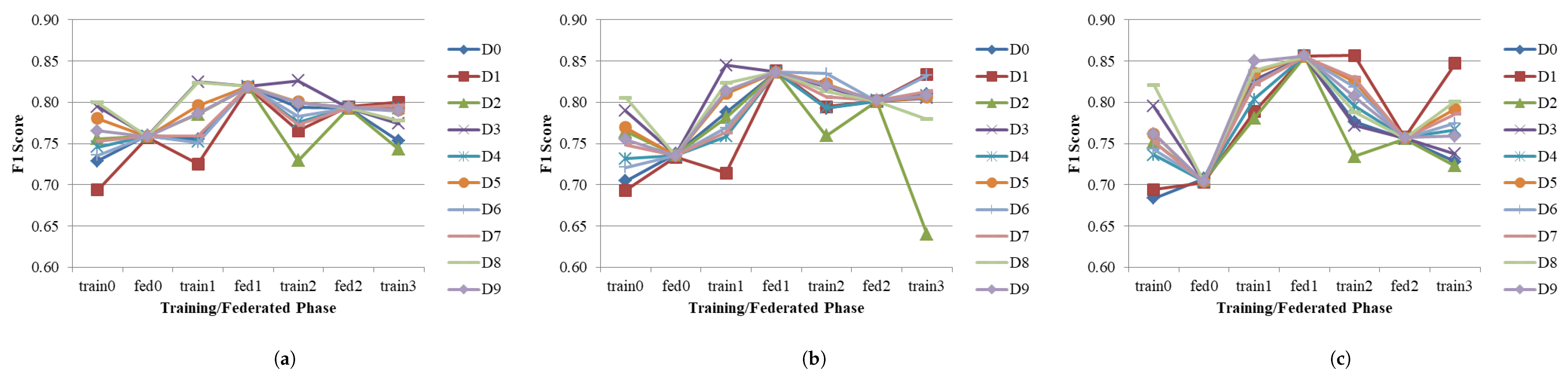
- Scenario 1 (Non-IID—Single Digit per Device): Each device was assigned images of a single digit from MNIST—e.g., device 0 trained on digit ‘0’, device 1 on digit ‘1’, and so on—covering all ten digit classes. This setup represents an extreme case of non-IID data distribution.
- Scenario 2 (IID—Partitioned Dataset): Each device received a distinct subset of the MNIST dataset containing all ten digit classes but with no overlap between subsets. This scenario investigates two aspects:
- –
- Training on Distinct MNIST Subsets: We evaluated how well the global model learns when devices are trained on disjoint partitions of the dataset.
- –
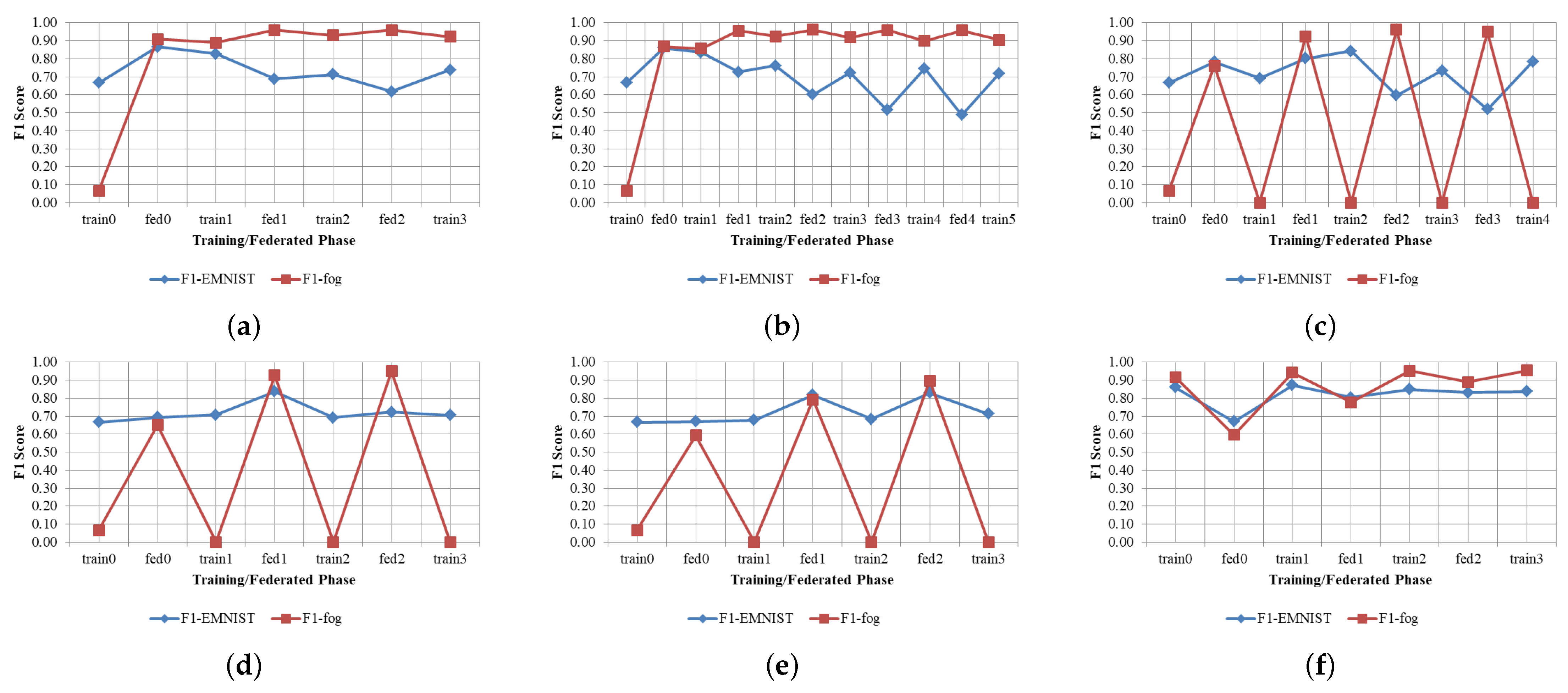
- Robustness to Anomalous Training Data: Selected devices were provided with corrupted training samples instead of regular MNIST, allowing us to assess the global model’s resilience in the presence of local data contamination.
5.1. Non-IID—Single Digit per Device
| Algorithm 1 Non-IID Partitioning: Single Digit per Device |
| Require: MNIST dataset with 10,000 samples 1: for each digit label to 9 do 2: Initialize empty list selected_samples 3: for each sample in do 4: if then 5: Append to selected_samples 6: end if 7: end for 8: Save selected_samples as a new dataset for the device assigned digit d 9: end for |
5.2. IID—Partitioned Dataset
5.2.1. Training on Distinct MNIST Subsets
5.2.2. Robustness to Anomalous Training Data
6. Resource Utilization Analysis
6.1. Program and Memory Footprint
6.2. Dataset Allocation in PSRAM
6.3. Model and Training Memory Usage
- Activations (A): Neuron values from the forward pass must be stored for backpropagation:
- Gradients: Gradients of the loss are accumulated during backpropagation. This requires the same number of float values as the model parameters: P floats.
- Neuron activation function derivative buffers: During backpropagation, these buffers temporarily store the derivatives of the activation functions for each neuron. Their size matches the number of neurons in each hidden and output layer:
- Optimizer state (Adam): Two additional floats per parameter (first and second moment estimates), totaling floats.
7. Experimental Results and Analysis
7.1. Evaluation of AutoencoderPerformance on PC

| Parameter | Value | Usage |
|---|---|---|
| Activation function | ReLU | Defines neuron output behavior |
| Optimizer | Adam | Adaptive weight updates |
| Learning rate | 0.001 | Step size for updates |
| Loss function | MSE | Measures prediction error |
| Patience phase 1 | 20 | Dual-phase early stopping |
| Patience phase 2 | 3 | Dual-phase early stopping |
| Acceptable loss | 0.02 | Dual-phase early stopping |
| Min delta | 0.0005 | Dual-phase early stopping |
| AD threshold function | 95th percentile | AD thresholding |
| gamma | 0.1 | AD thresholding (FL) |
| Patience phase 1 (FL) | 20 | Dual-phase early stopping (FL) |
| Patience phase 2 (FL) | 0 | Dual-phase early stopping (FL) |
| Acceptable loss (FL) | 0.02 | Dual-phase early stopping (FL) |
| Min delta (FL) | 0.0005 | Dual-phase early stopping (FL) |
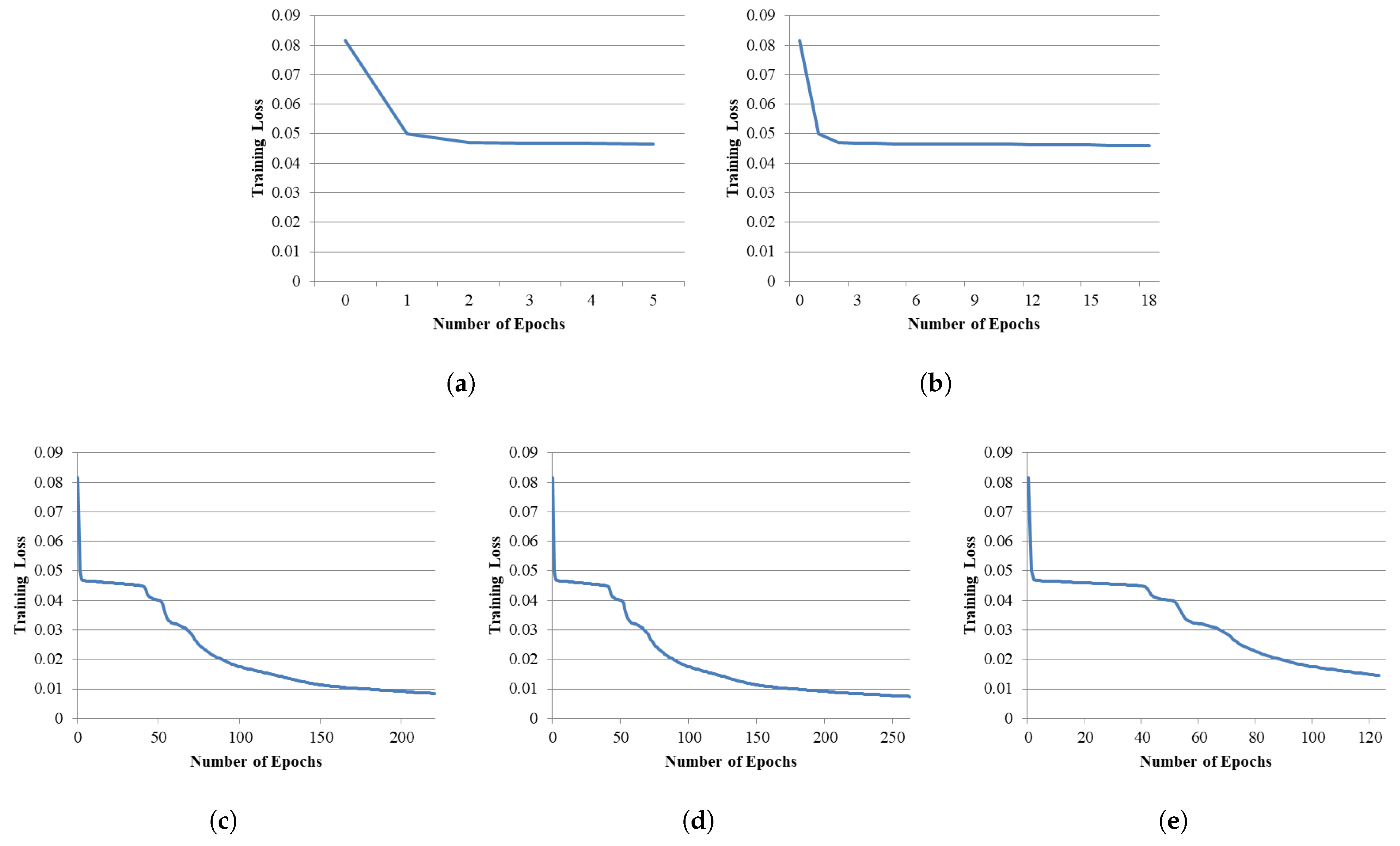
7.2. Evaluating the Dual-Phase Early Stopping Mechanism
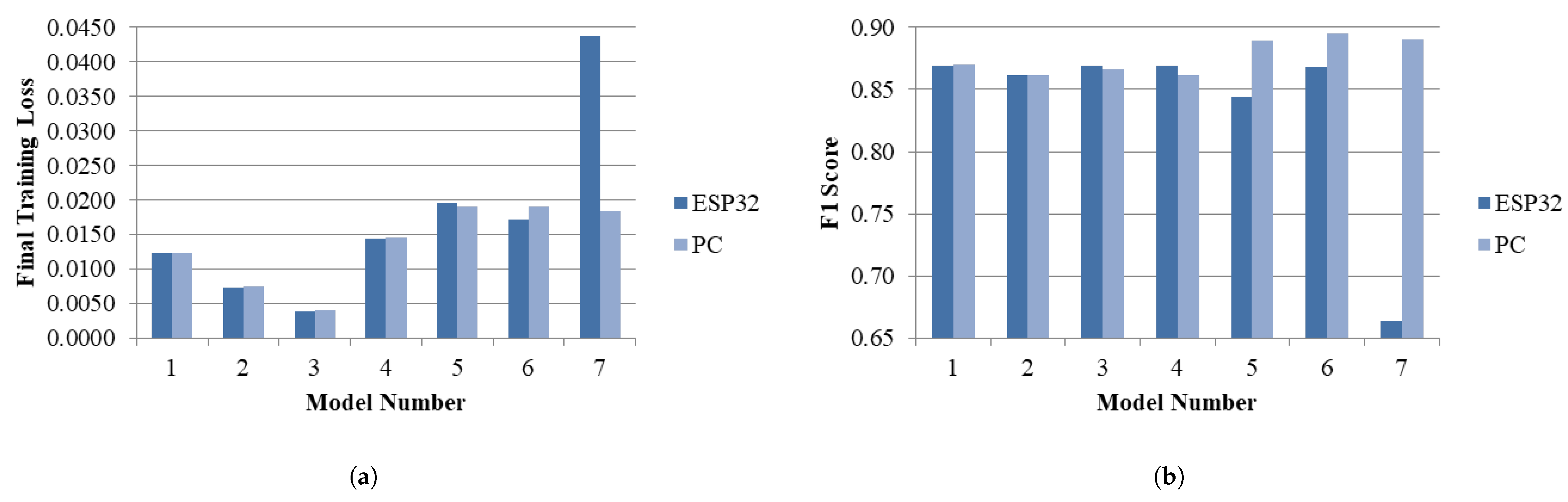
7.3. Evaluation of Autoencoder Performance on ESP32-CAM: Embedded Deployment
7.4. Federated Learning Scenario 1: Non-IID—Single Digit per Device
- Training time—to reduce energy consumption and improve convergence speed during FL rounds.
- Inference time—if real-time detection is critical.
- Memory footprint—for devices with severe RAM/Flash limitations.
- Model 1: Single hidden layer with 16 neurons—architecture: [196, 16, 196].
- Model 2: Single hidden layer with 32 neurons—architecture: [196, 32, 196].
- Model 3: Single hidden layer with 64 neurons—architecture: [196, 64, 196].
7.5. Federated Learning Scenario 2: IID—Partitioned Dataset
7.5.1. Training on Distinct MNIST Subsets
7.5.2. Robustness to Anomalous Training Data
- Configuration 1: devices 0–8 trained on clean MNIST; device 9 trained on fog.
- Configuration 2: devices 0–7 on MNIST; devices 8–9 on fog.
- Configuration 3: devices 0–6 on MNIST; devices 7–9 on fog.
- Configuration 4: devices 0–5 on MNIST; devices 6–9 on fog.
- Configuration 5: devices 0–4 on MNIST; devices 5–9 on fog.
7.6. Time Analysis of Federated Learning Workflow
7.7. Comparison with Other Approaches
8. Conclusions
Author Contributions
Funding
Data Availability Statement
Conflicts of Interest
Abbreviations
| ML | Machine Learning |
| FL | Federated Learning |
| IoT | Internet of Things |
| AE | Autoencoder |
| MCU | Microcontroller |
| AD | Anomaly Detection |
| PC | Personal Computer |
| IID | Independent and Identically Distributed |
| RAM | Random Access Memory |
| PSRAM | Pseudostatic RAM |
References
- David, R.; Duke, J.; Jain, A.; Janapa Reddi, V.; Jeffries, N.; Li, J.; Kreeger, N.; Nappier, I.; Natraj, M.; Wang, T.; et al. Tensorflow lite micro: Embedded machine learning for tinyml systems. Proc. Mach. Learn. Syst. 2021, 3, 800–811. [Google Scholar]
- Abadade, Y.; Temouden, A.; Bamoumen, H.; Benamar, N.; Chtouki, Y.; Hafid, A.S. A Comprehensive Survey on TinyML. IEEE Access 2023, 11, 96892–96922. [Google Scholar] [CrossRef]
- Tsoukas, V.; Gkogkidis, A.; Boumpa, E.; Kakarountas, A. A Review on the emerging technology of TinyML. ACM Comput. Surv. 2024, 56, 1–37. [Google Scholar] [CrossRef]
- Rajapakse, V.; Karunanayake, I.; Ahmed, N. Intelligence at the Extreme Edge: A Survey on Reformable TinyML. ACM Comput. Surv. 2023, 55, 1–30. [Google Scholar] [CrossRef]
- Ravindran, S. Cutting AI Down to Size. Science 2025, 387, 818–821. [Google Scholar] [CrossRef]
- Prakash, S.; Stewart, M.; Banbury, C.; Mazumder, M.; Warden, P.; Plancher, B.; Reddi, V.J. Is TinyML Sustainable? Commun. ACM 2023, 66, 68–77. [Google Scholar] [CrossRef]
- Vu, T.H.; Tu, N.H.; Huynh-The, T.; Lee, K.; Kim, S.; Voznak, M.; Pham, Q.V. Integration of TinyML and LargeML: A Survey of 6G and Beyond. arXiv 2025, arXiv:2505.15854. [Google Scholar]
- Trilles, S.; Hammad, S.S.; Iskandaryan, D. Anomaly detection based on artificial intelligence of things: A systematic literature mapping. Internet Things 2024, 25, 101063. [Google Scholar] [CrossRef]
- Le, D.K.; Nguyen, X.L. Lightweight Unsupervised Model for Anomaly Detection on Microcontroller Platforms. J. Marit. Res. 2024, 21, 187–195. [Google Scholar]
- Yap, Y.S.; Ahmad, M.R. Modified Overcomplete Autoencoder for Anomaly Detection Based on TinyML. IEEE Sens. Lett. 2024, 8, 1–4. [Google Scholar] [CrossRef]
- Geyer, R.C.; Klein, T.; Nabi, M. Differentially private federated learning: A client level perspective. arXiv 2017, arXiv:1712.07557. [Google Scholar]
- Kairouz, P.; McMahan, H.B.; Avent, B.; Bellet, A.; Bennis, M.; Bhagoji, A.N.; Bonawitz, K.; Charles, Z.; Cormode, G.; Cummings, R.; et al. Advances and Open Problems in Federated Learning. Found. Trends® Mach. Learn. 2021, 14, 1–210. [Google Scholar] [CrossRef]
- Zhang, T.; Gao, L.; He, C.; Zhang, M.; Krishnamachari, B.; Avestimehr, A.S. Federated learning for the internet of things: Applications, challenges, and opportunities. IEEE Internet Things Mag. 2022, 5, 24–29. [Google Scholar] [CrossRef]
- da Silva, C.N.; Prazeres, C.V.S. Tiny Federated Learning for Constrained Sensors: A Systematic Literature Review. IEEE Sens. Rev. 2025, 2, 17–31. [Google Scholar] [CrossRef]
- de Albuquerque Filho, J.E.; Brandao, L.C.; Fernandes, B.J.T.; Maciel, A.M. A review of neural networks for anomaly detection. IEEE Access 2022, 10, 112342–112367. [Google Scholar] [CrossRef]
- Ghamry, F.M.; El-Banby, G.M.; El-Fishawy, A.S.; El-Samie, F.E.A.; Dessouky, M.I. A survey of anomaly detection techniques. J. Opt. 2024, 53, 756–774. [Google Scholar] [CrossRef]
- Carannante, G.; Dera, D.; Aminul, O.; Bouaynaya, N.C.; Rasool, G. Self-assessment and robust anomaly detection with bayesian deep learning. In Proceedings of the 2022 25th International Conference on Information Fusion (FUSION), Linköping, Sweden, 4–7 July 2022; pp. 1–8. [Google Scholar]
- Denouden, T.; Salay, R.; Czarnecki, K.; Abdelzad, V.; Phan, B.; Vernekar, S. Improving reconstruction autoencoder out-of-distribution detection with Mahalanobis distance. arXiv 2018, arXiv:1812.02765. [Google Scholar]
- Ruff, L.; Vandermeulen, R.A.; Franks, B.J.; Müller, K.R.; Kloft, M. Rethinking assumptions in deep anomaly detection. arXiv 2020, arXiv:2006.00339. [Google Scholar]
- Haider, Z.A.; Zeb, A.; Rahman, T.; Singh, S.K.; Akram, R.; Arishi, A.; Ullah, I. A Survey on anomaly detection in IoT: Techniques, challenges, and opportunities with the integration of 6G. Comput. Netw. 2025, 270, 111484. [Google Scholar] [CrossRef]
- Capogrosso, L.; Cunico, F.; Cheng, D.S.; Fummi, F.; Cristani, M. A Machine Learning-Oriented Survey on Tiny Machine Learning. IEEE Access 2024, 12, 23406–23426. [Google Scholar] [CrossRef]
- Zeeshan, M. Efficient Deep Learning Models for Edge IOT Devices-A Review. Authorea Prepr. 2024. [Google Scholar] [CrossRef]
- Naveen, S.; Kounte, M.R. Optimized Convolutional Neural Network at the IoT edge for image detection using pruning and quantization. Multimed. Tools Appl. 2025, 84, 5435–5455. [Google Scholar] [CrossRef]
- Ghamari, S.; Ozcan, K.; Dinh, T.; Melnikov, A.; Carvajal, J.; Ernst, J.; Chai, S. Quantization-guided training for compact tinyml models. arXiv 2021, arXiv:2103.06231. [Google Scholar]
- Lin, J.; Chen, W.M.; Lin, Y.; Gohn, J.; Gan, C.; Han, S. Mcunet: Tiny deep learning on iot devices. Adv. Neural Inf. Process. Syst. 2020, 33, 11711–11722. [Google Scholar]
- Kim, D.; Yang, H.; Chung, M.; Cho, S.; Kim, H.; Kim, M.; Kim, K.; Kim, E. Squeezed convolutional variational autoencoder for unsupervised anomaly detection in edge device industrial internet of things. In Proceedings of the 2018 International Conference on Information and Computer Technologies (ICICT), DeKalb, IL, USA, 23–25 March 2018; pp. 67–71. [Google Scholar]
- Givnan, S.; Chalmers, C.; Fergus, P.; Ortega-Martorell, S.; Whalley, T. Anomaly detection using autoencoder reconstruction upon industrial motors. Sensors 2022, 22, 3166. [Google Scholar] [CrossRef]
- Bratu, D.V.; Ilinoiu, R.Ş.T.; Cristea, A.; Zolya, M.A.; Moraru, S.A. Anomaly Detection Using Edge Computing AI on Low Powered Devices. In Proceedings of the IFIP International Conference on Artificial Intelligence Applications and Innovations, Crete, Greece, 17–20 June 2022; pp. 96–107. [Google Scholar]
- Moallemi, A.; Burrello, A.; Brunelli, D.; Benini, L. Exploring scalable, distributed real-time anomaly detection for bridge health monitoring. IEEE Internet Things J. 2022, 9, 17660–17674. [Google Scholar] [CrossRef]
- Luo, T.; Nagarajan, S.G. Distributed anomaly detection using autoencoder neural networks in WSN for IoT. In Proceedings of the 2018 IEEE International Conference on Communications (ICC), Kansas City, MO, USA, 20–24 May 2018; pp. 1–6. [Google Scholar]
- Kwon, Y.D.; Li, R.; Venieris, S.I.; Chauhan, J.; Lane, N.D.; Mascolo, C. TinyTrain: Resource-aware task-adaptive sparse training of DNNs at the data-scarce edge. arXiv 2023, arXiv:2307.09988. [Google Scholar]
- Deutel, M.; Hannig, F.; Mutschler, C.; Teich, J. On-Device Training of Fully Quantized Deep Neural Networks on Cortex-M Microcontrollers. IEEE Trans. Comput.-Aided Des. Integr. Circuits Syst. 2025, 44, 1250–1261. [Google Scholar] [CrossRef]
- Ren, H.; Anicic, D.; Runkler, T.A. Tinyol: Tinyml with online-learning on microcontrollers. In Proceedings of the 2021 International Joint Conference on Neural Networks (IJCNN), Shenzhen, China, 18–22 July 2021; pp. 1–8. [Google Scholar]
- Abbasi, S.; Famouri, M.; Shafiee, M.J.; Wong, A. OutlierNets: Highly compact deep autoencoder network architectures for on-device acoustic anomaly detection. Sensors 2021, 21, 4805. [Google Scholar] [CrossRef]
- Qi, P.; Chiaro, D.; Piccialli, F. Small models, big impact: A review on the power of lightweight Federated Learning. Future Gener. Comput. Syst. 2024, 162, 107484. [Google Scholar] [CrossRef]
- Kopparapu, K.; Lin, E.; Breslin, J.G.; Sudharsan, B. Tinyfedtl: Federated transfer learning on ubiquitous tiny iot devices. In Proceedings of the 2022 IEEE International Conference on Pervasive Computing and Communications Workshops and Other Affiliated Events (PerCom Workshops), Pisa, Italy, 21–25 March 2022; pp. 79–81. [Google Scholar]
- Ficco, M.; Guerriero, A.; Milite, E.; Palmieri, F.; Pietrantuono, R.; Russo, S. Federated learning for IoT devices: Enhancing TinyML with on-board training. Inf. Fusion 2024, 104, 102189. [Google Scholar] [CrossRef]
- Nikić, V.; Bortnik, D.; Lukić, M.; Vukobratović, D.; Mezei, I. Lightweight Digit Recognition in Smart Metering System Using Narrowband Internet of Things and Federated Learning. Future Internet 2024, 16, 402. [Google Scholar] [CrossRef]
- Ren, H.; Anicic, D.; Runkler, T.A. TinyReptile: TinyML with federated meta-learning. In Proceedings of the 2023 International Joint Conference on Neural Networks (IJCNN), Gold Coast, Australia, 18–23 June 2023; pp. 1–9. [Google Scholar]
- Novoa-Paradela, D.; Fontenla-Romero, O.; Guijarro-Berdiñas, B. Fast deep autoencoder for federated learning. Pattern Recognit. 2023, 143, 109805. [Google Scholar] [CrossRef]
- Liu, X.; Su, X.; Campo, G.D.; Cao, J.; Fan, B.; Saavedra, E.; Santamaría, A.; Röning, J.; Hui, P.; Tarkoma, S. Federated Learning on 5G Edge for Industrial Internet of Things. IEEE Netw. 2025, 39, 289–297. [Google Scholar] [CrossRef]
- Reis, M.J. Edge-FLGuard: A Federated Learning Framework for Real-Time Anomaly Detection in 5G-Enabled IoT Ecosystems. Appl. Sci. 2025, 15, 6452. [Google Scholar] [CrossRef]
- Olanrewaju-George, B.; Pranggono, B. Federated learning-based intrusion detection system for the internet of things using unsupervised and supervised deep learning models. Cyber Secur. Appl. 2025, 3, 100068. [Google Scholar] [CrossRef]
- Ochiai, H.; Nishihata, R.; Tomiyama, E.; Sun, Y.; Esaki, H. Detection of global anomalies on distributed iot edges with device-to-device communication. In Proceedings of the Twenty-Fourth International Symposium on Theory, Algorithmic Foundations, and Protocol Design for Mobile Networks and Mobile Computing, Washington, DC, USA, 23–26 October 2023; pp. 388–393. [Google Scholar]
- Ai-Thinker Technology Co., Ltd. ESP32-CAM Schematic Diagram. Available online: https://docs.ai-thinker.com/_media/esp32/docs/esp32_cam_sch.pdf (accessed on 23 May 2025).
- LeCun, Y.; Bottou, L.; Bengio, Y.; Haffner, P. Gradient-based learning applied to document recognition. Proc. IEEE 1998, 86, 2278–2324. [Google Scholar] [CrossRef]
- Cohen, G.; Afshar, S.; Tapson, J.; van Schaik, A. EMNIST: Extending MNIST to handwritten letters. In Proceedings of the 2017 International Joint Conference on Neural Networks (IJCNN), Anchorage, AK, USA, 14–19 May 2017; pp. 2921–2926. [Google Scholar] [CrossRef]
- Mu, N.; Gilmer, J. MNIST-C: A Robustness Benchmark for Computer Vision. arXiv 2019, arXiv:1906.02337. [Google Scholar]
- TensorFlow. TensorFlow Datasets. Available online: https://www.tensorflow.org/datasets (accessed on 23 May 2025).
- TensorFlow. EarlyStopping Callback. Available online: https://www.tensorflow.org/api_docs/python/tf/keras/callbacks/EarlyStopping (accessed on 3 June 2025).
- Abadi, M.; Barham, P.; Chen, J.; Chen, Z.; Davis, A.; Dean, J.; Devin, M.; Ghemawat, S.; Irving, G.; Isard, M.; et al. {TensorFlow}: A system for {Large-Scale} machine learning. In Proceedings of the 12th USENIX Symposium on Operating Systems Design and Implementation (OSDI 16), Savannah, GA, USA, 2–4 November 2016; pp. 265–283. [Google Scholar]
- McMahan, B.; Moore, E.; Ramage, D.; Hampson, S.; y Arcas, B.A. Communication-efficient learning of deep networks from decentralized data. In Proceedings of the 20th International Conference on Artificial Intelligence and Statistics, Fort Lauderdale, FL, USA, 20–22 April 2017; pp. 1273–1282. [Google Scholar]
- Benmalek, M.; Benrekia, M.A.; Challal, Y. Security of federated learning: Attacks, defensive mechanisms, and challenges. Rev. Des Sci. Technol. L’Inf.-Série RIA Rev. D’Intelligence Artif. 2022, 36, 49–59. [Google Scholar] [CrossRef]
- Alsulaimawi, Z. Federated Learning with Anomaly Detection via Gradient and Reconstruction Analysis. arXiv 2024, arXiv:2403.10000. [Google Scholar]
- Allouah, Y.; Guerraoui, R.; Gupta, N.; Jellouli, A.; Rizk, G.; Stephan, J. Adaptive gradient clipping for robust federated learning. arXiv 2024, arXiv:2405.14432. [Google Scholar]
- Zhang, Z.; Cao, X.; Jia, J.; Gong, N.Z. Fldetector: Defending federated learning against model poisoning attacks via detecting malicious clients. In Proceedings of the 28th ACM SIGKDD Conference on Knowledge Discovery and Data Mining, Washington, DC, USA, 14–18 August 2022; pp. 2545–2555. [Google Scholar]
- Tanović, A.; Mezei, I. Embedded Parallel K-Means Algorithm Evaluation on ESP32 Across Various Memory Allocations. In Proceedings of the 2024 IEEE East-West Design & Test Symposium (EWDTS), Yerevan, Armenia, 13–17 November 2024; pp. 1–7. [Google Scholar]
| Model | Architecture | Inference Memory (KB) | Training Memory (KB) |
|---|---|---|---|
| Model 1 | [196, 16, 196] | 25.33 | 103.73 |
| Model 2 | [196, 32, 196] | 49.89 | 202.11 |
| Model 3 | [196, 64, 196] | 99.02 | 398.86 |
| Model 4 | [196, 32, 32, 196] | 54.02 | 218.86 |
| Model 5 | [196, 32, 8, 32, 196] | 52.05 | 211.05 |
| Model 6 | [196, 64, 16, 64, 196] | 107.33 | 432.73 |
| Model 7 | [196, 64, 32, 32, 64, 196] | 119.52 | 481.86 |
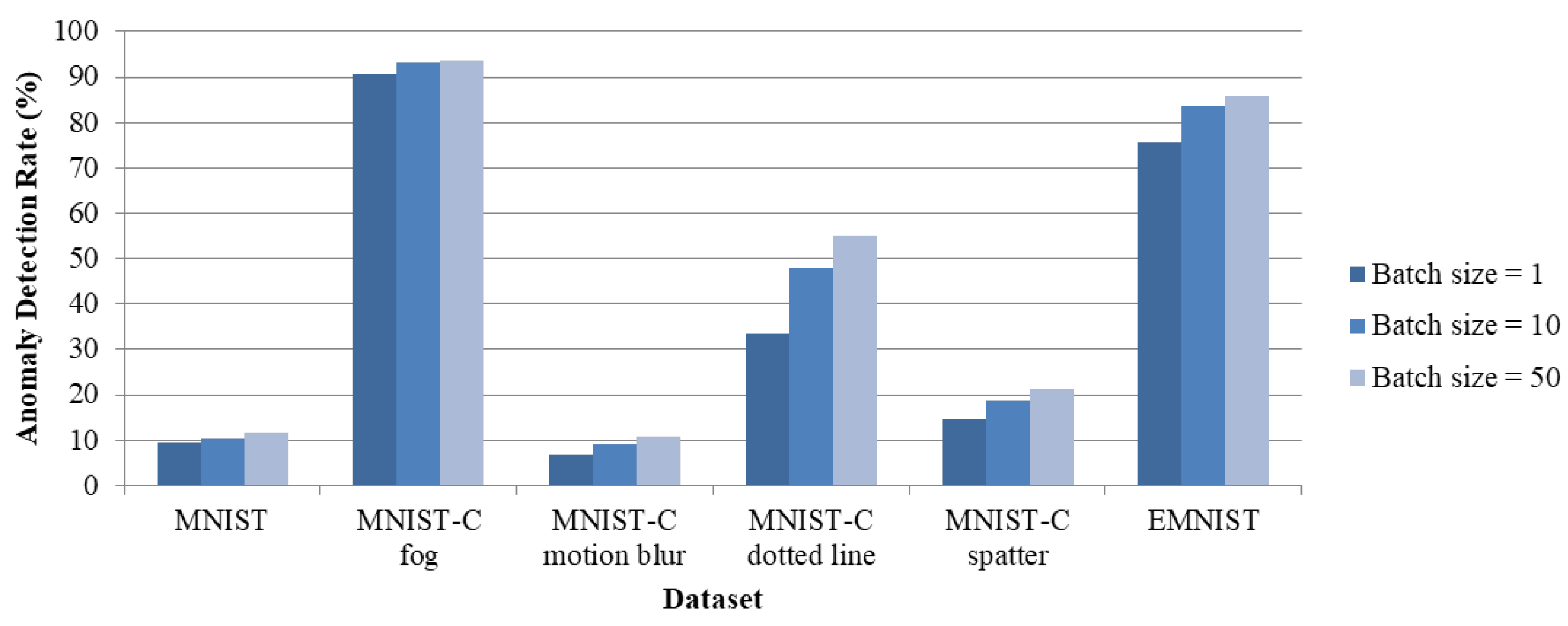
| Model Number | Training Configuration | Training Results | Anomaly Detection Rate (%) | F1 Score | |||||||||
|---|---|---|---|---|---|---|---|---|---|---|---|---|---|
| Autoencoder Architecture | Batch Size | Epochs | Final Training Loss | Training Time (s) | Inference Time (ms) | MNIST | MNIST-C Fog | MNIST-C Motion Blur | MNIST-C Dotted Line | MNIST-C Spatter | EMNIST | ||
| 1 | [196, 16, 196] | 1 | 11 | 0.0159 | 13.67 | 1.06 | 9.55 | 90.70 | 6.85 | 33.40 | 14.55 | 75.70 | 0.8173 |
| 10 | 26 | 0.0122 | 4.96 | 10.40 | 93.30 | 9.05 | 48.00 | 18.75 | 83.45 | 0.8610 | |||
| 50 | 60 | 0.0124 | 4.50 | 11.60 | 93.65 | 10.60 | 55.05 | 21.20 | 85.90 | 0.8699 | |||
| 2 | [196, 32, 196] | 1 | 13 | 0.0109 | 16.30 | 1.13 | 8.50 | 91.90 | 6.35 | 25.55 | 12.05 | 69.25 | 0.7792 |
| 10 | 29 | 0.0065 | 5.10 | 13.90 | 98.15 | 21.30 | 81.50 | 33.05 | 85.90 | 0.8599 | |||
| 50 | 61 | 0.0074 | 4.57 | 17.35 | 97.95 | 23.90 | 87.90 | 41.30 | 88.75 | 0.8612 | |||
| 3 | [196, 64, 196] | 1 | 16 | 0.0087 | 20.07 | 1.24 | 7.50 | 92.15 | 6.80 | 24.20 | 10.60 | 66.45 | 0.7640 |
| 10 | 30 | 0.0040 | 5.37 | 11.40 | 99.05 | 26.80 | 90.10 | 37.10 | 85.15 | 0.8664 | |||
| 50 | 53 | 0.0057 | 4.15 | 14.40 | 98.15 | 21.80 | 89.25 | 36.15 | 84.95 | 0.8523 | |||
| 4 | [196, 32, 32, 196] | 1 | 32 | 0.0122 | 68.04 | 1.31 | 9.60 | 92.90 | 7.65 | 36.10 | 15.20 | 75.80 | 0.8177 |
| 10 | 58 | 0.0119 | 18.01 | 14.10 | 95.00 | 14.70 | 63.20 | 26.00 | 86.35 | 0.8616 | |||
| 50 | 124 | 0.0146 | 12.49 | 12.55 | 91.70 | 12.60 | 51.30 | 21.25 | 86.80 | 0.8708 | |||
| 5 | [196, 32, 8, 32, 196] | 1 | 48 | 0.0188 | 134.42 | 1.33 | 11.85 | 88.40 | 9.95 | 38.80 | 18.90 | 86.95 | 0.8747 |
| 10 | 94 | 0.0191 | 30.97 | 12.05 | 89.20 | 10.30 | 41.55 | 17.80 | 89.80 | 0.8898 | |||
| 50 | 83 | 0.0437 | 6.36 | 6.35 | 63.20 | 0.80 | 15.55 | 4.75 | 51.30 | 0.6508 | |||
| 6 | [196, 64, 16, 64, 196] | 1 | 37 | 0.0139 | 105.63 | 1.38 | 12.55 | 90.75 | 12.85 | 42.40 | 21.55 | 87.25 | 0.8734 |
| 10 | 75 | 0.0145 | 24.79 | 15.70 | 93.80 | 20.00 | 56.55 | 28.65 | 90.25 | 0.8764 | |||
| 50 | 164 | 0.0191 | 15.16 | 11.30 | 88.70 | 11.40 | 37.60 | 16.25 | 90.25 | 0.8956 | |||
| 7 | [196, 64, 32, 32, 64, 196] | 1 | 47 | 0.0169 | 141.89 | 1.34 | 17.05 | 91.35 | 19.15 | 48.40 | 26.15 | 93.20 | 0.8866 |
| 10 | 107 | 0.0183 | 27.75 | 12.50 | 89.30 | 12.50 | 42.15 | 19.05 | 90.30 | 0.8905 | |||
| 50 | 115 | 0.0424 | 9.18 | 7.20 | 67.80 | 1.30 | 18.85 | 6.20 | 57.70 | 0.6998 | |||
| Strategy | Epochs | Anomaly Detection Rate (%) | F1 Score | |
|---|---|---|---|---|
| MNIST | EMNIST | |||
| Standard (patience = 3) | 6 | 6.25 | 47.00 | 0.6134 |
| Standard (patience = 10) | 19 | 6.45 | 48.05 | 0.6220 |
| Standard (patience = 15) | 221 | 19.25 | 91.30 | 0.8673 |
| Standard (patience = 20) | 263 | 21.45 | 91.75 | 0.8607 |
| Dual-phase (3/20) | 124 | 12.55 | 86.80 | 0.8708 |
| Model Number | Training Configuration | Training Results | Anomaly Detection Rate (%) | F1 Score | |||||||||
|---|---|---|---|---|---|---|---|---|---|---|---|---|---|
| Autoencoder Architecture | Batch Size | Epochs | Final Training Loss | Training Time (s) | Inference Time (ms) | MNIST | MNIST-C Fog | MNIST-C Motion Blur | MNIST-C Dotted Line | MNIST-C Spatter | EMNIST | ||
| 1 | [196, 16, 196] | 50 | 60 | 0.0124 | 727.18 | 9.34 | 11.50 | 93.65 | 10.30 | 54.30 | 20.95 | 85.65 | 0.8689 |
| 2 | [196, 32, 196] | 50 | 61 | 0.0074 | 1720.17 | 16.41 | 17.10 | 97.95 | 23.55 | 87.60 | 40.90 | 88.55 | 0.8612 |
| 3 | [196, 64, 196] | 10 | 30 | 0.0038 | 2547.34 | 32.21 | 11.95 | 99.10 | 27.25 | 91.20 | 37.90 | 86.00 | 0.8689 |
| 4 | [196, 32, 32, 196] | 50 | 115 | 0.0144 | 3558.55 | 21.49 | 11.35 | 91.65 | 11.25 | 46.45 | 18.75 | 85.65 | 0.8695 |
| 5 | [196, 32, 8, 32, 196] | 10 | 111 | 0.0196 | 3577.33 | 16.47 | 12.30 | 88.20 | 7.85 | 33.35 | 15.15 | 81.95 | 0.8438 |
| 6 | [196, 64, 16, 64, 196] | 50 | 158 | 0.0172 | 12618.32 | 35.48 | 12.30 | 88.80 | 11.20 | 42.35 | 18.10 | 86.10 | 0.8679 |
| 7 | [196, 64, 32, 32, 64, 196] | 10 | 42 | 0.0437 | 4281.15 | 42.07 | 6.90 | 62.60 | 0.85 | 14.55 | 5.05 | 53.10 | 0.6638 |
| Training/Federated Phase | Anomaly Detection Rate (%) | F1 Score ± | |||||||||||||||||||
|---|---|---|---|---|---|---|---|---|---|---|---|---|---|---|---|---|---|---|---|---|---|
| Digit 0 | Digit 1 | Digit 2 | Digit 3 | Digit 4 | Digit 5 | Digit 6 | Digit 7 | Digit 8 | Digit 9 | ||||||||||||
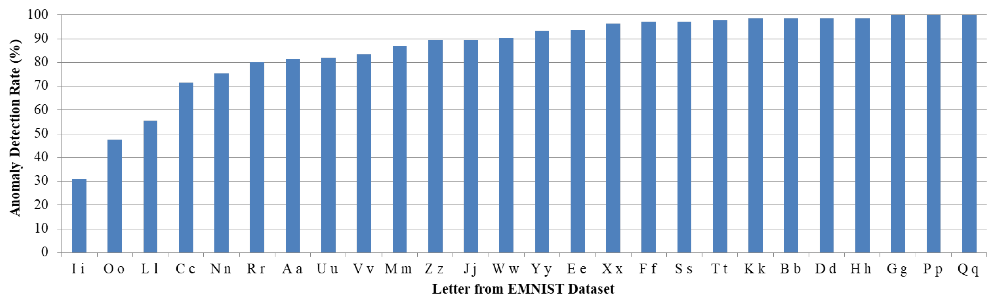
| MNIST | EMNIST | MNIST | EMNIST | MNIST | EMNIST | MNIST | EMNIST | MNIST | EMNIST | MNIST | EMNIST | MNIST | EMNIST | MNIST | EMNIST | MNIST | EMNIST | MNIST | EMNIST | ||
| train0 | 84.90 | 96.05 | 88.20 | 100.00 | 59.60 | 96.15 | 48.85 | 98.20 | 68.05 | 97.85 | 59.05 | 97.80 | 65.00 | 97.50 | 64.25 | 99.05 | 35.50 | 94.35 | 61.65 | 99.45 | 0.75 ± 0.0410 |
| fed0 | 82.40 | 99.80 | 84.35 | 99.85 | 83.20 | 99.85 | 83.70 | 99.85 | 83.70 | 99.85 | 83.85 | 99.85 | 83.30 | 99.85 | 83.85 | 99.85 | 83.75 | 99.85 | 83.90 | 99.85 | 0.70 ± 0.0013 |
| train1 | 15.45 | 81.30 | 50.25 | 97.80 | 7.15 | 68.60 | 7.35 | 75.60 | 28.40 | 86.30 | 23.80 | 88.75 | 24.10 | 86.85 | 25.45 | 87.45 | 12.90 | 81.50 | 18.20 | 87.35 | 0.82 ± 0.0220 |
| fed1 | 8.95 | 81.45 | 9.30 | 81.80 | 8.95 | 81.45 | 9.05 | 81.50 | 9.10 | 81.60 | 9.10 | 81.60 | 9.05 | 81.50 | 9.05 | 81.50 | 9.05 | 81.50 | 9.10 | 81.70 | 0.86 ± 0.0003 |
| train2 | 4.05 | 66.05 | 17.45 | 88.00 | 3.15 | 59.85 | 3.00 | 64.70 | 7.40 | 70.95 | 9.15 | 76.65 | 4.45 | 72.35 | 9.35 | 77.55 | 5.75 | 68.80 | 5.60 | 71.45 | 0.80 ± 0.0349 |
| fed2 | 1.80 | 61.85 | 1.90 | 62.15 | 1.80 | 61.85 | 1.80 | 61.90 | 1.80 | 62.00 | 1.80 | 62.00 | 1.80 | 61.90 | 1.80 | 61.90 | 1.80 | 61.90 | 1.80 | 62.00 | 0.76 ± 0.0006 |
| train3 | 1.90 | 58.30 | 8.25 | 79.55 | 1.80 | 57.65 | 1.70 | 59.40 | 3.00 | 64.05 | 4.95 | 68.80 | 1.85 | 64.35 | 4.75 | 67.80 | 5.85 | 70.75 | 2.45 | 62.65 | 0.77 ± 0.0378 |
| Training/Federated Phase | Final Training Loss | Anomaly Detection Rate (%) | F1 Score | |||||
|---|---|---|---|---|---|---|---|---|
| MNIST | MNIST-C Fog | MNIST-C Motion Blur | MNIST-C Dotted Line | MNIST-C Spatter | EMNIST | |||
| train0 | 0.0098 | 12.65 | 95.25 | 14.90 | 66.85 | 25.25 | 85.25 | 0.8615 |
| fed0 | - | 9.50 | 93.95 | 11.05 | 51.55 | 18.45 | 84.80 | 0.8729 |
| train1 | 0.0051 | 1.70 | 94.45 | 3.85 | 17.10 | 2.55 | 60.15 | 0.7433 |
| fed1 | - | 0.90 | 94.40 | 2.25 | 11.70 | 1.20 | 56.15 | 0.7151 |
| train2 | 0.0037 | 0.80 | 94.45 | 2.40 | 7.60 | 0.95 | 49.35 | 0.6573 |
| fed2 | - | 0.50 | 94.50 | 1.40 | 5.55 | 0.50 | 45.70 | 0.6252 |
| train3 | 0.0034 | 0.65 | 94.45 | 1.95 | 5.40 | 0.75 | 45.15 | 0.6193 |
| fed3 | - | 0.50 | 94.40 | 0.95 | 4.90 | 0.50 | 42.55 | 0.5949 |
| train4 | 0.0036 | 0.60 | 94.50 | 1.60 | 5.05 | 0.70 | 43.75 | 0.6062 |
| Training/Federated Phase | Configuration 1 | Configuration 2 | Configuration 3 | Configuration 4 | Configuration 5 | |||||
|---|---|---|---|---|---|---|---|---|---|---|
| F1-EMNIST | F1-Fog | F1-EMNIST | F1-Fog | F1-EMNIST | F1-Fog | F1-EMNIST | F1-Fog | F1-EMNIST | F1-Fog | |
| train0 | 0.8437 ± 0.0631 | 0.8382 ± 0.2710 | 0.8250 ± 0.0840 | 0.7530 ± 0.3593 | 0.8038 ± 0.0950 | 0.6651 ± 0.4158 | 0.7839 ± 0.1012 | 0.5783 ± 0.4456 | 0.7664 ± 0.1052 | 0.4927 ± 0.4558 |
| fed0 | 0.8720 ± 0.0020 | 0.8996 ± 0.0038 | 0.8457 ± 0.0076 | 0.8467 ± 0.0113 | 0.7584 ± 0.0176 | 0.7385 ± 0.0167 | 0.6897 ± 0.0036 | 0.6492 ± 0.0018 | 0.6707 ± 0.0002 | 0.5943 ± 0.0027 |
| train1 | 0.7726 ± 0.0218 | 0.9584 ± 0.0243 | 0.8012 ± 0.0212 | 0.9456 ± 0.0464 | 0.7790 ± 0.0626 | 0.6771 ± 0.4672 | 0.7808 ± 0.0821 | 0.5766 ± 0.4963 | 0.7675 ± 0.1012 | 0.4731 ± 0.4987 |
| fed1 | 0.7381 ± 0.0176 | 0.9620 ± 0.0008 | 0.7627 ± 0.0190 | 0.9578 ± 0.0006 | 0.8157 ± 0.0092 | 0.9229 ± 0.0017 | 0.8417 ± 0.0043 | 0.9223 ± 0.0047 | 0.8111 ± 0.0075 | 0.7859 ± 0.0081 |
| train2 | 0.7018 ± 0.0242 | 0.9646 ± 0.0119 | 0.7149 ± 0.0373 | 0.9638 ± 0.0203 | 0.7394 ± 0.0658 | 0.6846 ± 0.4724 | 0.7491 ± 0.0553 | 0.5840 ± 0.5026 | 0.7747 ± 0.0815 | 0.4788 ± 0.5047 |
| fed2 | 0.6642 ± 0.0164 | 0.9659 ± 0.0019 | 0.6480 ± 0.0256 | 0.9653 ± 0.0023 | 0.6412 ± 0.0316 | 0.9666 ± 0.0029 | 0.7473 ± 0.0214 | 0.9511 ± 0.0008 | 0.8311 ± 0.0012 | 0.8936 ± 0.0041 |
| train3 | 0.6498 ± 0.0326 | 0.9648 ± 0.0151 | 0.6558 ± 0.0453 | 0.9617 ± 0.0232 | 0.6473 ± 0.0592 | 0.6851 ± 0.4728 | 0.7368 ± 0.0354 | 0.5838 ± 0.5025 | 0.7993 ± 0.0610 | 0.4785 ± 0.5044 |
| fed3 | - | - | 0.5729 ± 0.0303 | 0.9651 ± 0.0031 | 0.5584 ± 0.0268 | 0.9532 ± 0.0023 | - | - | - | - |
| train4 | - | - | 0.6255 ± 0.0678 | 0.9558 ± 0.0314 | 0.6227 ± 0.1050 | 0.6832 ± 0.4714 | - | - | - | - |
| fed4 | - | - | 0.5384 ± 0.0271 | 0.9635 ± 0.0030 | - | - | - | - | - | - |
| train5 | - | - | 0.5976 ± 0.0661 | 0.9561 ± 0.0277 | - | - | - | - | - | - |
| Work | Device Type | Device (RAM/Frequency) | Model Type | Model Size | Inference Latency | On-Device Train | FL |
|---|---|---|---|---|---|---|---|
| [26] | - | - | SCVAE | 12 MB | 6 ms | - | - |
| [27] | - | - | Stacked AE | - | - | - | - |
| [28] | ESP32 | 520 KB/240 MHz | AE | - | - | - | - |
| [29] | STM32L476 | 128 KB/80 MHz | PCA, AE, Conv-AE | 77.55 KB, -, - | 6.428 ms, -, - | - | - |
| [30] | - | - | AE | - | - | - | - |
| [33] | Arduino Nano 33 BLE Sense | 256 KB/64 MHz | AE | - | - | ✓, OL | - |
| [34] | i5-7600K, ARM Cortex A72 | -/3.8 GHz, 4 GB/1.5 GHz | Deep Conv-AE | 2.7–273 KB | 0.366–0.746 s, 6.044–13.575 s | ✓ | - |
| [40] | i7-11700K | 64 GB/3.6 GHz | Deep AE for FL | - | - | ✓ | ✓ |
| [41] | i7-8700K, NVIDIA GeForce RTX 2080 Max-Q | 32 GB/3.7 GHz, 8 GB GPU | LSTM AE | - | - | ✓ | ✓ |
| [42] | Raspberry Pi 4, Jetson Nano | 4 GB/1.5 GHz, 4 GB GPU | AE, LSTM | 29 MB, 42 MB | 13.1 ms, 19.6 ms | ✓ | ✓ |
| [44] | - | - | WAFL-AE | - | - | ✓ | ✓ |
| [43] | - | - | AE, DNN | - | - | ✓ | ✓ |
| This work | ESP32-CAM | 520 KB/240 MHz | AE | 25–120 KB | 9–42 ms | ✓ | ✓ |
Disclaimer/Publisher’s Note: The statements, opinions and data contained in all publications are solely those of the individual author(s) and contributor(s) and not of MDPI and/or the editor(s). MDPI and/or the editor(s) disclaim responsibility for any injury to people or property resulting from any ideas, methods, instructions or products referred to in the content. |
© 2025 by the authors. Licensee MDPI, Basel, Switzerland. This article is an open access article distributed under the terms and conditions of the Creative Commons Attribution (CC BY) license (https://creativecommons.org/licenses/by/4.0/).
Share and Cite
Tanović, A.; Mezei, I. Lightweight Anomaly Detection in Digit Recognition Using Federated Learning. Future Internet 2025, 17, 343. https://doi.org/10.3390/fi17080343
Tanović A, Mezei I. Lightweight Anomaly Detection in Digit Recognition Using Federated Learning. Future Internet. 2025; 17(8):343. https://doi.org/10.3390/fi17080343
Chicago/Turabian StyleTanović, Anja, and Ivan Mezei. 2025. "Lightweight Anomaly Detection in Digit Recognition Using Federated Learning" Future Internet 17, no. 8: 343. https://doi.org/10.3390/fi17080343
APA StyleTanović, A., & Mezei, I. (2025). Lightweight Anomaly Detection in Digit Recognition Using Federated Learning. Future Internet, 17(8), 343. https://doi.org/10.3390/fi17080343