A Robust Conformal Framework for IoT-Based Predictive Maintenance

Abstract

This study, set within the vast and varied research field of industrial Internet of Things (IoT) systems, proposes a methodology to address uncertainty quantification (UQ) issues in predictive maintenance (PdM) practices. At its core, this paper leverages the commercial modular aero-propulsion system simulation (CMAPSS) dataset to evaluate different artificial intelligence (AI) prognostic algorithms for remaining useful life (RUL) forecasting while supporting the estimation of a robust confidence interval (CI). The methodology primarily involves the comparison of statistical learning (SL), machine learning (ML), and deep learning (DL) techniques for each different scenario of the CMAPSS, evaluating the performances through a tailored metric, the S-score metric, and then benchmarking diverse conformal-based uncertainty estimation techniques, remarkably naive, weighted, and bootstrapping, offering a more suitable and reliable alternative to classical RUL prediction. The results obtained highlight the peculiarities and benefits of the conformal approach, despite probabilistic models favoring the adoption of complex models in cases where the operating conditions of the machine are multiple, and suggest the use of weighted conformal practices in non-exchangeability conditions while recommending bootstrapping alternatives for contexts with a more substantial presence of noise in the data.

1. Introduction

In today’s Industry 4.0 landscape, equipment, processes, and decision support systems (DSS) are seamlessly interconnected, with a vast amount of sensor data continuously collected in real time. This interconnectivity facilitates various applications (e.g., predictive maintenance), ultimately transforming traditional manufacturing into agile, data-driven systems. The IoT plays a pivotal role in this technological shift, utilizing sensor displacements and platforms to connect devices and gather data seamlessly, enabling intelligent analytics through AI. According to Bonomi et al. [1], IoT facilitates the structuring of complex ecosystems, enabling data processing through five distinct layers (sensing, network, storage, learning, and application). The comprehensive review by Killeen and Parvizimosaed [2] also supports the structured logic mentioned by Bonomi, highlighting the crucial functions of the layers in the IoT pipeline, from the data source to the extraction of information. In most IoT architectures, the sensing layer gathers data through sensors and actuators, representing the physical part of the system, and disseminates data through the network layer, which extends the computation to other apparatuses such as cloud or fog systems. Then, the storage layer is responsible for caching and preserving data, while the learning layer employs information retrieval through advanced algorithms or data analysis. The DSS is supported by the application layer. It utilizes the valuable insight presented in a human-interpretable way to enhance practical applications or to be integrated into larger systems (e.g., networking, security, intelligent IoT). Although the layered IoT architecture mentioned above is relevant in many domains (from medical to agriculture), it is particularly beneficial when adopted in critical domains where timing responsiveness is pivotal (e.g., industrial maintenance). PdM, clearly born from the combination of AI and IoT, represents the paradigm shift from traditional maintenance strategies. The adoption of data-driven methodologies permits the forecasting of a system’s future state, ergo estimating the machine degradation pattern (prognosis) [3,4]. Conversely, this intelligent approach allows more complex anomaly detection methodologies (diagnosis) while seeking to optimize maintenance schedules, reduce unplanned downtime, and minimize production costs.

Historically, this transformation originated from the past industrial revolutions. It commenced with simple strategies, such as reactive maintenance based on visual inspections by trained craftsmen and preventive maintenance based on planned routine operations, scheduled inspections, and performance monitoring [5]. In the last century, condition-based monitoring (CbM) appeared as a pioneering data-driven approach to more effectively monitoring the health and performance of machinery through sensors. It emerged as a branch of mechanical engineering, as highlighted in the seminal work by Den [6], and then was embraced as a branch of statistics, emphasizing the importance of data analysis in maintenance decision-making processes [7]. The operational deployment of this approach involves several critical steps, with parameter selection representing a pivotal stage to identify the most relevant variables indicating the condition of the machinery [8]. By processing the set of selected parameters, it is possible to generate potential condition indicators that represent the statistical properties of the process by providing quantifiable measures of equipment health [9]. Subsequently, quality control charts, baselines, and thresholds are set for monitoring deviations from normal operating conditions [10]. In practice, the later stage involves statistical techniques to determine these control limits, identifying regions of in-control conditions, thereby highlighting abnormal behavior in the alternative machinery’s performance. The final phase of CbM comprises effective continuous monitoring with real-time data flow, intending to trigger alerts and maintenance actions when certain thresholds are exceeded [11], representing a comprehensive, data-driven management system. The CbM approach facilitates the construction of a diagnostic framework capable of timely fault detection, possibly minimizing sudden production interruptions, proactively identifying potential issues and root causes, allowing timely maintenance interventions, and enhancing the reliability and efficiency of manufacturing processes. The integration of modern and complex sensor apparatus has significantly improved the effectiveness of CbM techniques, enhancing the understanding of machinery health and contributing to operational efficiency, making these well-oiled strategies even more adaptable in the actual maintenance context; however, uncertainties inherent in analytics due to the more complex technological processes coupled with the time constraints under which decisions must be made pose significant challenges and limitations to its applicability. These limitations have catalyzed the development of PdM and its sophisticated variants, positioning them as innovative drivers for maintenance management systems promising to improve maintenance strategies and decision-making processes further.

Technically, the PdM strategies significantly depend on robust and reliable data flow. Through IoT platforms, the analytics can be conducted at the level of individual machines, manufacturing cells, factories, or across entire networks of factories via cloud solutions. However, these data sets are often fragmented across different systems and exist as isolated data islands, or “silos”, which feature varying semantics and formats, making them hardly interoperable and challenging to amalgamate within a PdM framework [12]. Christou et al. introduce a digital platform designed explicitly for PdM to address these challenges. This platform provides comprehensive support for implementing PdM applications, minimizing the effort required for deployment. The platform achieves this through middleware functions that streamline data collection, facilitate advanced data analytics, and complete the feedback loop by configuring other systems based on assets’ predictive insights [12].

Methodologically, the effectiveness of PdM systems relies heavily on the analytical capabilities provided by various data mining and machine learning techniques. These systems analyze datasets to derive predictive insights about the lifetime of assets, focusing on parameters such as RUL and time to end of life (EoL). Studies by Paolanti et al. (2018) explore the use of diverse machine learning methods in PdM, emphasizing their crucial role in the field [13]. In this context, neural networks have also been identified as particularly effective for these applications.

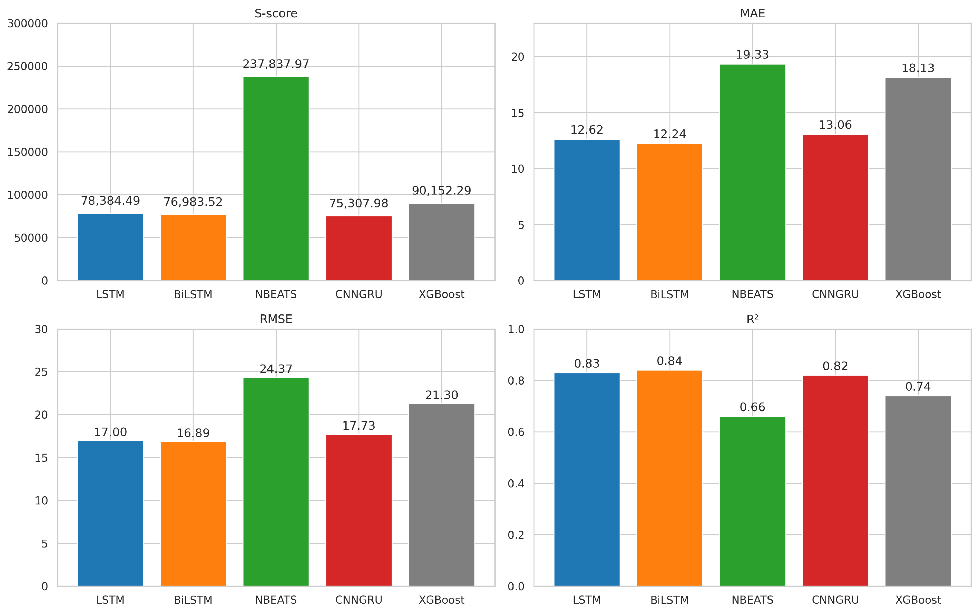
Generally, in the actual PdM research panorama, several algorithms and learning strategies have been utilized to predict the RUL [14], ranging from SL to DL architectures. Among the principal algorithms found in the literature, are statistical models such as Prophet [15], machine learning techniques like Extreme Gradient Boosting (XGBoost) [16], and other decision tree-based variants. Additionally, DL methodologies like Long Short-Term Memory (LSTM), Bidirectional LSTM (BiLSTM), Neural Basis Expansion Analysis for Time Series (N-BEATS), and Convolutional Neural Network-Gated Recurrent Unit (CNN-GRU) have been extensively applied, with significant contributions to PdM outcomes [17,18,19,20]. These approaches underscore the importance of selecting the correct algorithm based on the system and dataset’s characteristics. This is crucial, as the performance of these algorithms can significantly affect the accuracy of the RUL predictions and the overall efficiency of the maintenance strategy. However, data scarcity in PdM for critical systems such as aircraft engines is still a significant barrier to developing predictive models in real applications. In addressing this issue, Saxena et al. (2008) have contributed to the field by introducing the CMAPSS dataset [21] along with simulation paradigms and guidelines. This dataset, developed through damage propagation modeling for aircraft engine run-to-failure simulation, has become a pivotal resource for researchers and practitioners in the field of prognostics and health management, allowing for the realistic simulation and testing of PdM models and providing a vital tool at the disposal of the scientific community. Nonetheless, the field of PdM is still in need of more generalized AI research, as mentioned by Fink et al. (2020), which discusses the potential and challenges of deploying DL within prognostics and health management, emphasizing the need for future research to address the complex patterns in the data and effectively implement data-driven strategies [22]. Additionally, Tiddens et al. (2015) highlight the slow adoption rate of AI-powered prognostic strategies in decision-making, remarking on the significant gap between their potential benefits and their practical applications, highlighting the need for an intermediate framework that translates data into actionable maintenance decisions, offering more explicit guidance on practical maintenance actions [23].

While these areas have seen significant progress, a comprehensive methodological framework for reliable PdM tasks is still needed. Punctual or multi-horizon forecasting poses stringent limitations on the practical usage of the PdM algorithm in real-world conditions, both when integrated into larger optimization procedures (involving multiple components, plants, and other data sources) and even as an effective DSS serving engineers and domain experts. Moreover, sensor misreading, noise, and missingness can amplify the negative impact of these practices in a real setting, remarking the need for a more reliable solution that extends the algorithm’s forecasting power.

UQ has recently emerged as an interesting practice in time series analysis and forecasting. It refers to the unpredictability associated with future values of a data sequence due to various factors such as randomness, external influences, and incomplete information. Managing and quantifying uncertainty in time series forecasting is crucial for decision-making processes across diverse domains, including PdM, permitting the construction of a more sophisticated predictive framework that is even more essential when applied to industrial critical components or workflows. In this context, Conformal Prediction is established solidly among the most widely used techniques for estimating confidence intervals due to its practical potential (it does not require explicit assumptions about the predictive algorithm) and flexibility (it works without a predefined data distribution), opening a new potential era for refined DSS supplied by a reliable CI.

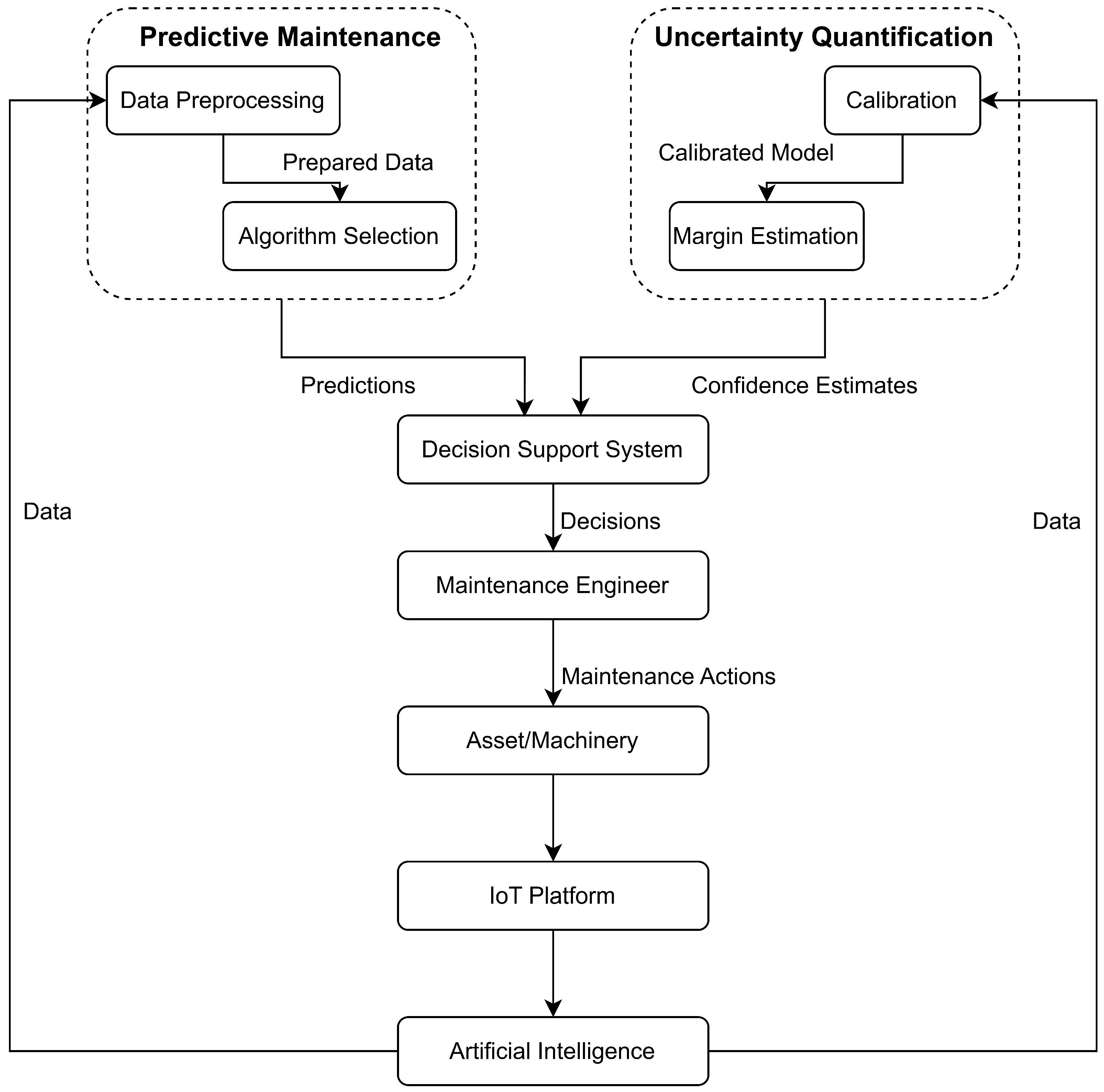
This work leverages a comprehensive overview that highlights the extensive development of research of IoT systems in PdM to offer a methodological approach to algorithm selection and CI evaluation, as presented in Figure 1, offering a tailored framework for robust IoT-enabled PdM, leading to more efficient and secure maintenance operations. In detail, the study aims to show that when sensor streams exhibit non-stationary behavior and the underlying degradation process is explicitly modeled, embedding a clamp-regulated, one-sided Conformal Prediction layer into the RUL-estimation pipeline produces statistically valid yet markedly tighter lower-bound uncertainty intervals than representative distribution-based benchmarks.

This manuscript is articulated in the following sections:

• Section 1 Introduction—motivation and problem statement
• Section 2 Time series analysis in predictive maintenance—survey of RUL models.
• Section 3 CI estimation in predictive maintenance—limits of current UQ methods.
• Section 4 CMAPSS dataset—benchmark dataset description.
• Section 5 Robust conformal prognostic for reliable predictive maintenance.
• Section 6 Experimental result and performance evaluation.
• Section 7 Discussion—practical IoT implications.
• Section 8 Conclusion—key findings and future work.

2. Time Series Analysis in Predictive Maintenance

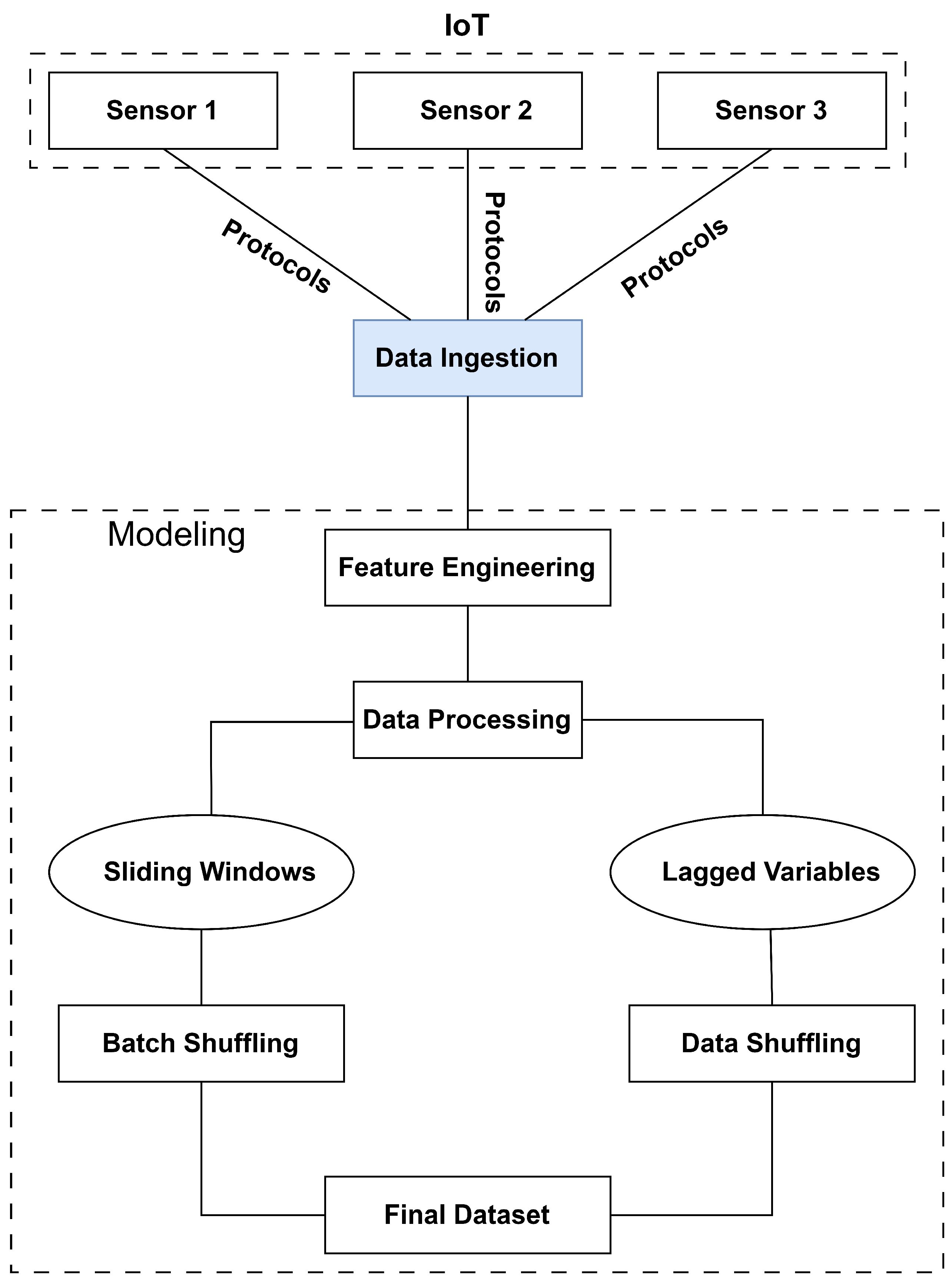
At the juncture between AI and IoT in the field of PdM, the data ensemble is the pivotal starting point in PdM data modeling by integrating historical and real-time data to form a rich dataset that underpins the PdM strategy. Through the meticulous data workflow presented in Figure 2, the IoT platforms offer sophisticated data processing techniques to synchronize and merge data flowing from multiple machines. Additionally, the platform ensures the applicability of AI models, which can access all necessary information for accurate prediction.

Through this comprehensive data structure, the development of predictive models that can accurately forecast potential machine failures using a time series analysis framework empowers organizations to make timely and informed maintenance decisions.

The last critical data processing step is transforming raw time series data into a format suitable for predictive analysis. The primary techniques utilized in this context are sliding windows and lagged variables. The sliding window technique processes time series data by employing a fixed-size window that traverses the data points sequentially, capturing contiguous subsets of the original series. Mathematically, given a time series $X=\{x_1,x_2,\dots ,x_n\}$ and a window size w, the subsets analyzed are presented in the following equations.

$$(x_i,x_{i+1},\dots ,x_{i+w-1}),\mathrm{for}\mathrm{each}i=1,\dots ,n-w+1$$

(1)

The choice of window size is critical since a too-small window might miss significant trends. In contrast, a window that is too large could oversmooth essential data fluctuations, so it should be adequately regulated by the previous correlation analysis. Similar to the sliding window, the lagged variables approach is also particularly practical in capturing the temporal dynamics. It works by shifting the time series backward by one or more periods, making it suitable for those predictive models that do not operate with a three-dimensional data batch structure. The process is mathematically described as:

$$X_{t-\mathrm{shift}}=\{x_{i-\mathrm{shift}}\mid i=1,\dots ,n\}$$

(2)

where shift is the number of periods the data is moved backward. This technique emphasizes shifting data feature-wise, offering an alternative to the three-dimensional data structure typically formed by the batches in the sliding window approach.

Focusing on the PdM practices, the main aim of this research is to predict the RUL with its progressive failure process. However, one principal peculiarity regarding PdM practices is the absence of a specific target value, as highlighted by [24]. Their work emphasizes that degradation modeling always relies on inferring the target variable from historical data rather than having explicit labels for failure events. Health prognostics is one of the core tasks in CBM, which aims to predict the RUL of machinery based on the historical and ongoing degradation trends observed through condition monitoring information [25,26,27].

In machinery, a prognostic program generally consists of four technical processes, i.e., data acquisition, health indicator (HI) construction, health stage (HS) division, and RUL prediction. It is crucial in PdM to model the target variable (e.g., RUL or degradation state), as this forms the foundation for training predictive models and establishing CI around the predictions. Among the various techniques of RUL extraction, linear modeling is often used in the early stages of RUL estimation, where degradation trends are generally used in simple linear assumptions. This linear degradation modeling can be refined through survival analysis, which provides a probabilistic framework for estimating the time until failure, defining an early RUL value, and then truncating the linear RUL value, defining “in-control regions”.

In PdM, survival analysis estimates how long a machine or its components will continue to operate effectively before failure. This estimation helps organizations plan maintenance activities proactively, thereby reducing downtime and extending the equipment’s lifespan. The Kaplan–Meier estimator, which measures the fraction of units operating over a certain amount of time without failure, provides a robust framework for understanding the machinery lifespan and failure rates.

$$\widehat{S}\left(t\right)=\prod _{t_i\le t}\left(1-{\displaystyle \frac{d_i}{n_i}}\right)$$

(3)

where $d_i$ is the number of failures observed, and $n_i$ is the number of units at risk at time $t_i$.

• Early RUL phase: initially, when a machine is new or has been recently maintained, the probability of failure is low, and thus, the RUL can be assumed to be relatively constant or decreasing very slowly.

  $$RUL\left(t\right)=R_{\mathrm{early}},\mathrm{for}t<T$$

  (4)
• Degradation phase: As the equipment ages and wear accumulates, the RUL decreases more rapidly. This phase can be modeled using a linear degradation function informed by the failure rates derived from the Kaplan–Meier analysis reaching the unit EoL.

  $$RUL\left(t\right)=R_{\mathrm{early}}-k·(t-T),\mathrm{for}t\ge T$$

  (5)

In the above formulation, T represents the transition time between the early RUL phase and the degradation phase, and k is a constant, calibrated based on historical data analyzed using the Kaplan–Meier estimator, that quantifies the degradation rate. By integrating survival analysis with the piecewise linear degradation functions, PdM models can more accurately estimate when machinery is likely to fail, not considering or learning patterns that are not probably presenting failure status but just focusing on the start of anomalous sensor drifts.

3. CI Estimation in Predictive Maintenance

In real-world situations, machine learning or AI applications are often incorrect or unreliable because of various factors, such as insufficient or incomplete data, issues arising during the modeling process, or simply the randomness and complexities of the underlying problem. These problems are critical in estimating the RUL and constructing intervals for prognostic outcomes.

CI presents a range of possible values derived from sample data, providing a measure of uncertainty around the prediction value that reflects the variability inherent in sampling [28]. CI estimation, presented in Equation (6), is divided into three key components: calibration, residual analysis, and margin estimation. Calibration involves adjusting or fine-tuning the model parameters to ensure the predictions align as closely as possible with the observed data, with the residual analysis focusing on examining the differences between the observed values and the model’s predicted values [29]. At the same time, margin estimation refers to calculating the range around the predicted value in which the actual value is expected to lie, given a certain confidence level. The formula for a CI is as follows:

$$CI=\widehat{\theta }\pm z·SE$$

(6)

where $\widehat{\theta }$ is the sample estimate, z represents the critical value corresponding to the desired confidence level, and $SE$ is the standard error of the estimate.

In classical statistical learning models, like ARIMA (Auto-Regressive Integrated Moving Average), CI is estimated based on the assumption that residuals are usually distributed by calculating the standard error of the forecast from the fitted model and estimating the CI by adding and subtracting the product of the critical value and the standard error from the predicted value [30]. In probabilistic frameworks like Prophet, CI is estimated using simulation over multiple possible future scenarios by sampling from the calibration distribution and using those simulated forecasts to compute empirical percentiles, defining the CI. In contrast, frameworks like CP present more flexible capabilities since they provide post-hoc uncertainty evaluation, adapting to any underlying forecasting model.

In the following part of this section, a detailed analysis of Prophet and Conformal strategy is presented, highlighting their internal workflows and remarking on the pros and cons when applied for uncertainty quantification in the domain of PdM.

3.1. Prophet

Prophet is an open-source forecasting tool developed by Facebook (now Meta) for time series data [31], designed to be easy to use, interpretable, and capable of handling common time series patterns such as trends, seasonality, and holidays. Principally, Prophet falls under the umbrella of the probabilistic paradigm, leveraging Bayesian posterior inference to estimate uncertainty in the forecast, not requiring forcing the time series into a stationary state (e.g., integrating the lags) and well-handling missingness and noise in the data. The time series for a piecewise linear multiplicative $y\left(t\right)$ prophet model can be shown in Equation (7):

$$y\left(t\right)=1\ast \left(g\right(t)\ast s(t)\ast h(t\left)\right)+ϵ\left(t\right)$$

(7)

where $ϵ\left(t\right)$ is the error term, and $g\left(t\right)$, $s\left(t\right)$, and $h\left(t\right)$ represent the trend, seasonal, and holiday terms.

• Trend component: The trend component is denoted as $g\left(t\right)$, which represents the non-periodic and long-term changes in the value of a time series. It captures the underlying pattern or direction of the data over time, excluding short-term fluctuations or seasonal variations. A piecewise linear function is a common approach to modeling $g\left(t\right)$, which estimates the trend as a series of connected linear segments. The mathematical formulation for $g\left(t\right)$ is presented through Equation (8):

  $$g\left(t\right)=(k+\mathbf{a}{\left(t\right)}^T\mathit{\delta })t+(m+\mathbf{a}{\left(t\right)}^T\mathit{\gamma })$$

  (8)

  where the following is true:

  −

  k: initial growth rate;

  −

  $\mathit{\delta }$: vector of rate adjustments at changepoints;

  −

  $\mathbf{a}\left(t\right)$: indicator vector for changepoints;

  −

  m: offset parameter;

  −

  $\mathit{\gamma }$: vector of offset adjustments at changepoints, defined as ${\gamma }_j=s_j{\delta }_j$.

• Seasonal component: The function $s\left(t\right)$ represents the seasonal component. It captures the seasonal effects in the data, such as daily, weekly, or yearly patterns. $s\left(t\right)$ uses a Fourier series to model these seasonal effects, a mathematical tool that decomposes periodic functions into a sum of sine and cosine terms. For seasonality modeling, the Fourier series is defined as in Equation (9).

  $$s\left(t\right)=\sum _{n=1}^N\left(a_{n}cos\left({\displaystyle \frac{2\pi nt}{P}}\right)+b_{n}sin\left({\displaystyle \frac{2\pi nt}{P}}\right)\right)$$

  (9)

  where the following is true:

  −

  N is the order of the Fourier series;

  −

  P is the period of the seasonality;

  −

  $a_n$ and $b_n$ are coefficients;

  −

  t is the time variable.

• Holidays component: The holiday component, denoted by $h\left(t\right)$. It models the effects of holidays or special events on the time series. Unlike regular seasonality, holidays often occur on irregular schedules and can significantly impact the data. To account for these effects, Prophet uses binary variables to indicate whether a given time point t falls on a holiday. Each holiday i is assigned a coefficient ${\kappa }_i$, quantifying its impact on the time series. The overall holidays component is then calculated as the sum of these effects for all relevant holidays. The mathematical expression for $h\left(t\right)$ is provided in the Equation (10).

  $$h\left(t\right)=\sum _i{\kappa }_i·\mathbb{I}(t\in {\mathrm{holiday}}_i)$$

  (10)

  where the following is true:

  −

  $h\left(t\right)$: holidays component at time t;

  −

  ${\kappa }_i$: coefficient representing the impact of holiday i;

  −

  $\mathbb{I}(t\in {\mathrm{holiday}}_i)$: indicator function that equals 1 if t falls on holiday i and 0 otherwise.

In Prophet, CI can be estimated using two primary approaches: Monte Carlo sampling and posterior predictive distributions. Monte Carlo sampling generates multiple future scenarios by randomly sampling from the model’s parameters, while posterior predictive distributions directly simulate forecasts based on the fitted model’s uncertainty. Then, these simulated forecasts are used to compute empirical percentiles (e.g., 95% CI corresponds to the 2.5th and 97.5th percentiles), which define the CI.

3.2. Conformal Prediction

CP is a robust machine learning framework that provides valid confidence measurements for individual predictions. Predictions made by ML or DL often come without the UQ, which is required for confident and reliable decision-making in the real world. Quantifying uncertainty is a prerequisite for explainability and trust in machine learning models. Using any model within the CP framework generates predictions and quantifies the confidence in those predictions. Several different approaches to quantifying uncertainty exist, such as statistical methods, Bayesian methods, and fuzzy logic methods [32].

Statistical methods are widely used for UQ and involve using probability distributions to model the uncertainty in data and prediction. Bayesian methods use prior knowledge and data to update beliefs about the uncertainty in predictions. Fuzzy logic involves using sets and membership functions to represent uncertainty in a system. Considering the CP framework, there are three primary approaches to estimating CI, such as NCP (Naive Conformal Prediction), BCP (Bootstrapping-Based Conformal Prediction), and WCP (Weighted Conformal Prediction) [33,34,35].

To perform CP, the first critical step is to calculate the nonconformity score, which measures how unusual or non-conforming the observed data are compared with the predicted values. Generally, it measures how much the model’s prediction deviates from reality. NCP is the most straightforward approach to estimating the nonconformity score. It computed the nonconformity score for each data point by the difference between observed values and predicted values. It is computed directly using this formula:

$$s_i=|Y_i-\widehat{f}\left(X_i\right)|$$

(11)

where $Y_i$ is the observed value for the i-th data point and $\widehat{f}\left(X_i\right)$ is the predicted value from the model for input $X_i$.

However, in BCP, the nonconformity score is calculated by resampling techniques. For each BCP sample b, the nonconformity score is computed by the same formula as in NCP. In BCP, multiple samples are generated from the original dataset. For each sample of BCP, the nonconformity score is calculated as the absolute difference between the predicted and observed values. The formula for calculating the nonconformity score of the BCP sample is

$$s_i^{\left(b\right)}=|Y_i-{\widehat{f}}^{\left(b\right)}\left(X_i\right)|$$

(12)

where ${\widehat{f}}^{\left(b\right)}\left(X_i\right)$ is the model trained on the i-th BCP sample.

The WCP is the extent of the NCP, which assigns weight $w_i$ to calibration points. By assigning weight $w_i$, the CP reflects the importance of the i-th calibration point (e.g., based on time proximity, relevance, or domain-specific knowledge). The formula for calculating the nonconformity score using weight is

$$s_i=w_i·|Y_i-\widehat{f}\left(X_i\right)|$$

(13)

where $w_i$ is the weight reflecting the relative importance.

After computing the nonconformity scores for the three different approaches—NCP, BCP, and WCP—the next step is to calculate the quantile threshold using the significance level $\alpha$. This threshold ensures that the CI achieves the desired coverage probability. The specific method for determining the threshold varies depending on the approach, but all rely on the $(1-\alpha )$-th quantile of the nonconformity scores.

In NCP, the quantile threshold is determined as

$$q_{1-\alpha }={\mathrm{quantile}}_{1-\alpha }\{s_1,s_2,\dots ,s_n\}$$

(14)

where $q_{1-\alpha }$ is the $(1-\alpha )$-th quantile of the calibration scores and $\{s_1,s_2,\dots ,s_n\}$ represents the set of nonconformity scores.

For BCP sample b, the quantile threshold is determined as

$$q_{1-\alpha }={\mathrm{quantile}}_{1-\alpha }\{s_1^{\left(1\right)},s_2^{\left(1\right)},\dots ,s_n^{\left(B\right)}\}$$

(15)

where B is the total number of BCP samples.

For WCP, the nonconformity score is calculated using the weight $w_i$. So, a weighted quantile is used to compute the threshold as follows:

$$q_{1-\alpha }={\mathrm{weighted}\text{\_}\mathrm{quantile}}_{1-\alpha }\{s_1,s_2,\dots ,s_n\}$$

(16)

where the weighted_quantile accounts for the relative importance of each score based on the assigned weights.

The final formula for computing the CI is the same for all three methods. To calculate the CI, include all candidate values Y that satisfy $s_{n+1}\le q_{1-\alpha }$, where $s_{n+1}$ is the nonconformity score for the new prediction and $q_{1-\alpha }$ is the quantile threshold computed differently depending on the methods as the following formula:

$$C\left(X_{n+1}\right)=\{Y:s_{n+1}\le q_{1-\alpha }\}$$

(17)

$$P(Y_{n+1}\in C_n\left(X_{n+1}\right))\ge 1-\alpha$$

(18)

This formula states that the probability of true response $Y_{n+1}$ falling within the predicted confidence set $C_n\left(X_{n+1}\right)$ is at least ($1-\alpha$).

From the performance evaluation perspective, the key metrics for CP are margin, coverage, and average width. Margin is defined as the quantile of the absolute errors or nonconformity scores, which is computed on a calibration set. If a score is taken from the target coverage percentile, then this score will be added to and subtracted from the point prediction to form the prediction interval. A higher margin result is always a wider interval, which represents the prediction intervals with more stability and reliability. In comparison, a lower margin generates narrow intervals that provide more precise estimates but are less robust. Coverage measures the robustness of the predicted interval. It refers to the proportion of times when the actual value falls within the predicted CI.

$$\mathrm{Coverage}={\displaystyle \frac{1}{N}}\sum _{i=1}^N\mathbf{1}\left\{y_i\in \left[max\{0,{\widehat{y}}_i-m\},{\widehat{y}}_i\right]\right\},$$

(19)

The coverage value is presented in Equation (19), where N is the total number of predictions, $\mathbf{1}\{·\}$ is the indicator function that evaluates to 1 if the condition is true (and 0 otherwise), and ${\widehat{y}}_i$ is the point prediction for the ith sample. The m is the margin, which determines how well the predicted intervals capture the actual value. Lowering the coverage value means that its prediction intervals often fail to capture the actual values. In contrast, a higher coverage value indicates that actual values fall within the prediction intervals. The average width measures the size of the predicted intervals. It is calculated simply as the mean of the widths of all prediction intervals. Narrower intervals are more precise but may sacrifice coverage, while wider intervals are less accurate but more reliable. The calibration set is central to this process. It is used to compute the nonconformity scores that define the margin, ensuring that the selected margin reflects the model’s performance on unseen data. This allows the integrity of the performance assessment to be maintained, as the metrics computed on the test set are not influenced by the margin selection process.

In the above sections, we have explained the Prophet and CP methodologies to compute CI for predicted values. It is visible that these two approaches have different patterns when calculating CI. Prophet incorporates seasonality, trends, and holidays through simulation-based methods (e.g., Monte Carlo sampling or posterior predictive distributions), while CP relies on nonconformity scores and quantile thresholds in different methods (e.g., NCP, BCP, and WCP) to perform CI even under non-exchangeability conditions and data drifts.

4. Commercial Modular Aeropropulsion Simulation System (CMAPSS) Dataset

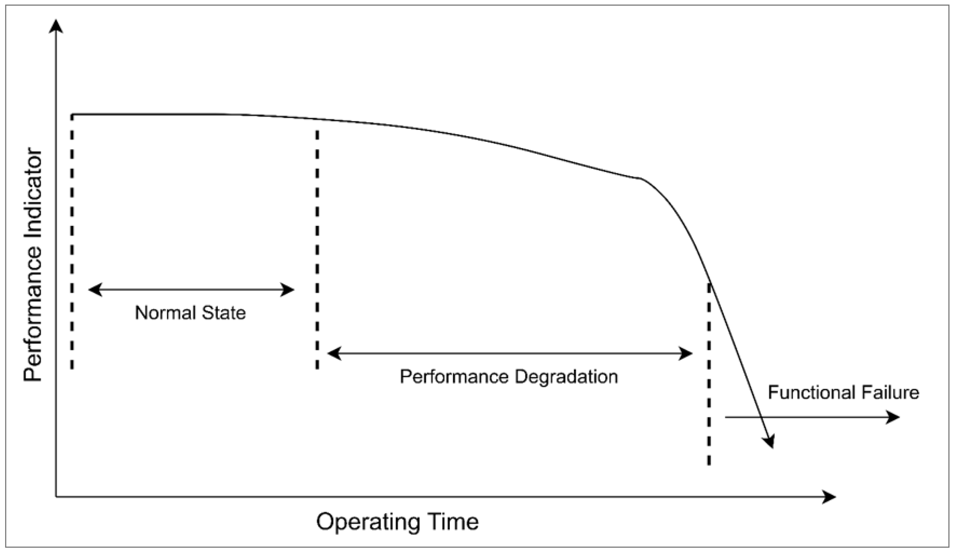
The CMAPSS simulated datasets [21], courtesy of the NASA Center of Excellence, represent a typical ensemble of a jet engine (turbofan) that operates with a faulty and complex wear system. This dataset presents a pivotal and trusted data source for diagnostic and prognostic analysis, allowing the RUL prediction of each separate unit, thereby modeling their specific and progressive failure processes. 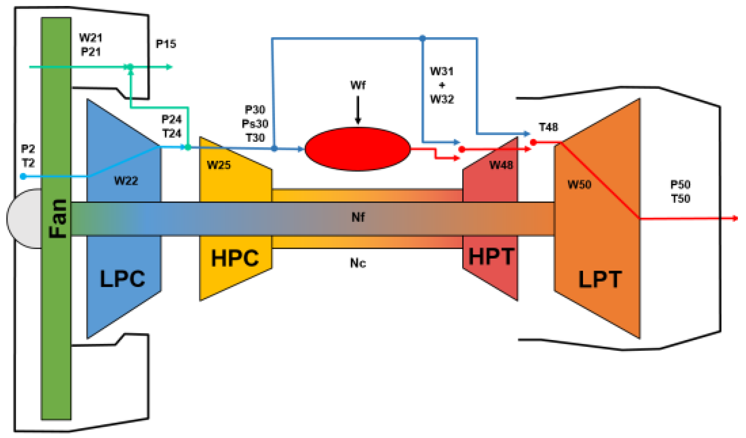Generally, engine failure refers to mechanical degradation resulting from variations in output sensor parameters caused by damage or wear, with its pattern following a typical evolutionary trajectory, which can be depicted by the curve shown in Figure 3. This curve illustrates the gradual decline in jet performance over time, supporting the analysis and prediction of engine RUL. Particularly, the CMAPSS software involves the simultaneous failures of up to five rotating sub-components, which are presented in Figure 4: fan, low-pressure compressor (LPC), high-pressure compressor (HPC), low-pressure turbine (LPT), and high-pressure turbine (HPT). In addition to component-level failures, the CMAPSS simulation environment incorporates various flight conditions that can significantly influence engine performance, including parameters such as altitude, Mach number, and throttle resolve angle (TRA), which permit more realistic modeling of a wide range of operational scenarios.

Other relevant variants of the CMAPSS have been proposed by Chao et al. [36], leveraging a more tailored and structured approach intended to represent a small fleet of aircraft better by taking advantage of the CMAPSS tool, which presents an extension of the original dataset but captures similar patterns and trends in the data, de facto incorporating its predecessor. The generation process adopted by the authors is presented in Algorithm 1.

Specifically, FD001 and FD002 consist of 100 engine units each, whereas FD003 and FD004 consist of 260 and 249 units, respectively. The specific measurements present various operational parameters, such as fuel flow, fan speed, and various temperatures and pressures throughout the turbofan engine system. These datasets could be mainly grouped into two classes, as presented in

Table 1. CMAPSS dataset overview.

Property	FD1	FD2	FD3	FD4
Engine units (train)	100	260	100	249
Operational conditions	1	6	1	6
Fault modes	1	1	2	2
Minimum lifespans (train)	128	128	146	128
Maximum lifespans (train)	362	378	526	544
Minimum cycles recorded (test)	31	21	38	19
Maximum cycles recorded (test)	303	367	475	486

:

• Single operational condition: FD1–FD3 presents a single working condition, indicating that the data were captured at specific flight settings (Mach, TRA, Altitude).
• Multiple operational condition: FD2–FD4 presents six working conditions, indicating that the data were captured at different flight settings (Mach, TRA, Altitude).

Algorithm 1: Generate Degradation Data

return Output time series of observables for each operational cycle (hours) [21].

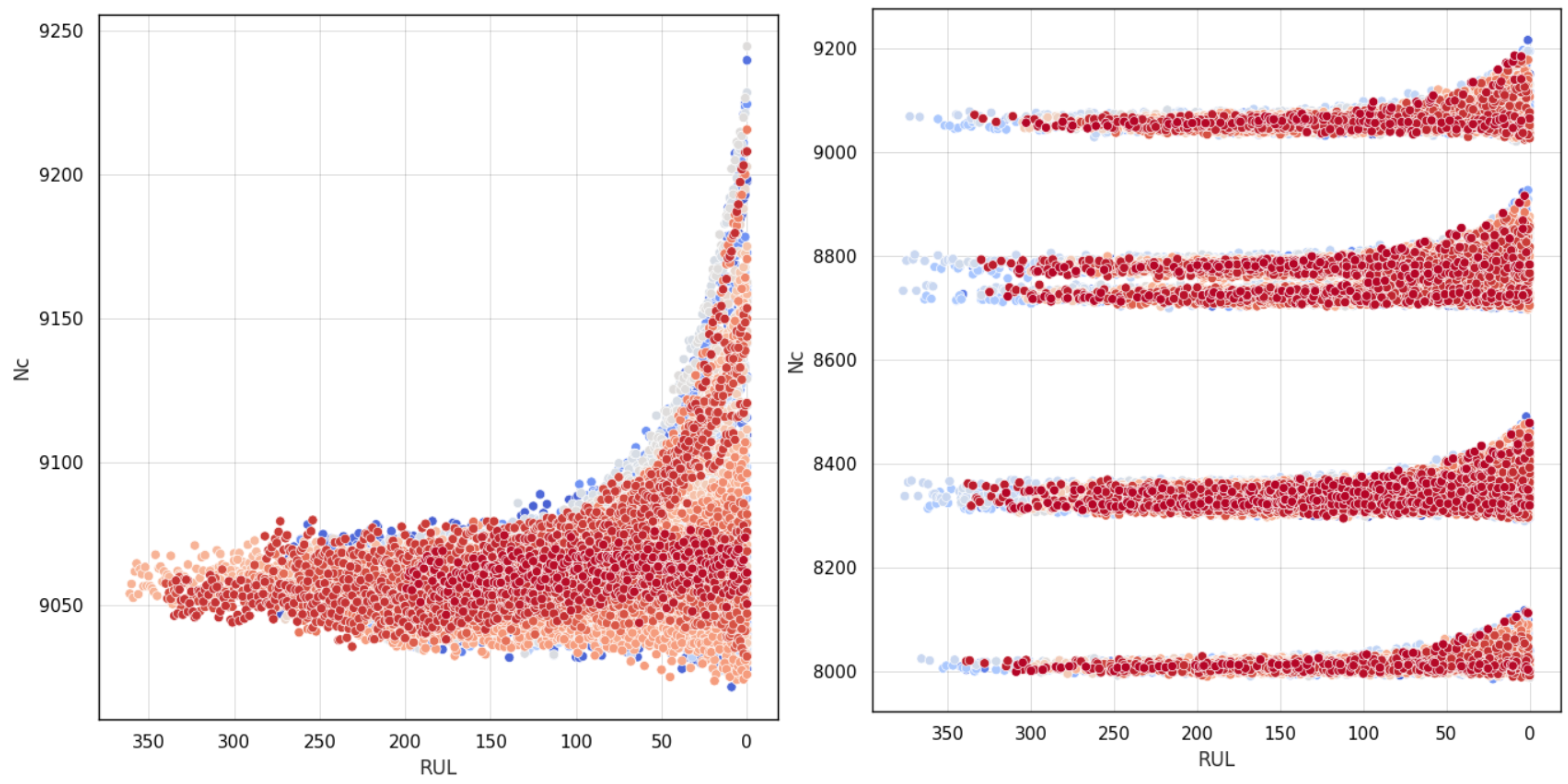
The main differences between these two classes of datasets can also be visually inspected through Figure 5. The FD1 dataset represents a singular failure modality and operational condition, while the FD2 dataset presents the same failure condition through different operational settings. In the above-mentioned figure of the RUL, presented on the axis, it is calculated following Equation (20). Basically, it represents the reverse of the number of cycles as hours [21], which is a known parameter that sets the granularity of the sensor series from the beginning till the EoL.

$$\mathrm{RUL}\left(t\right)=T-t+1.$$

(20)

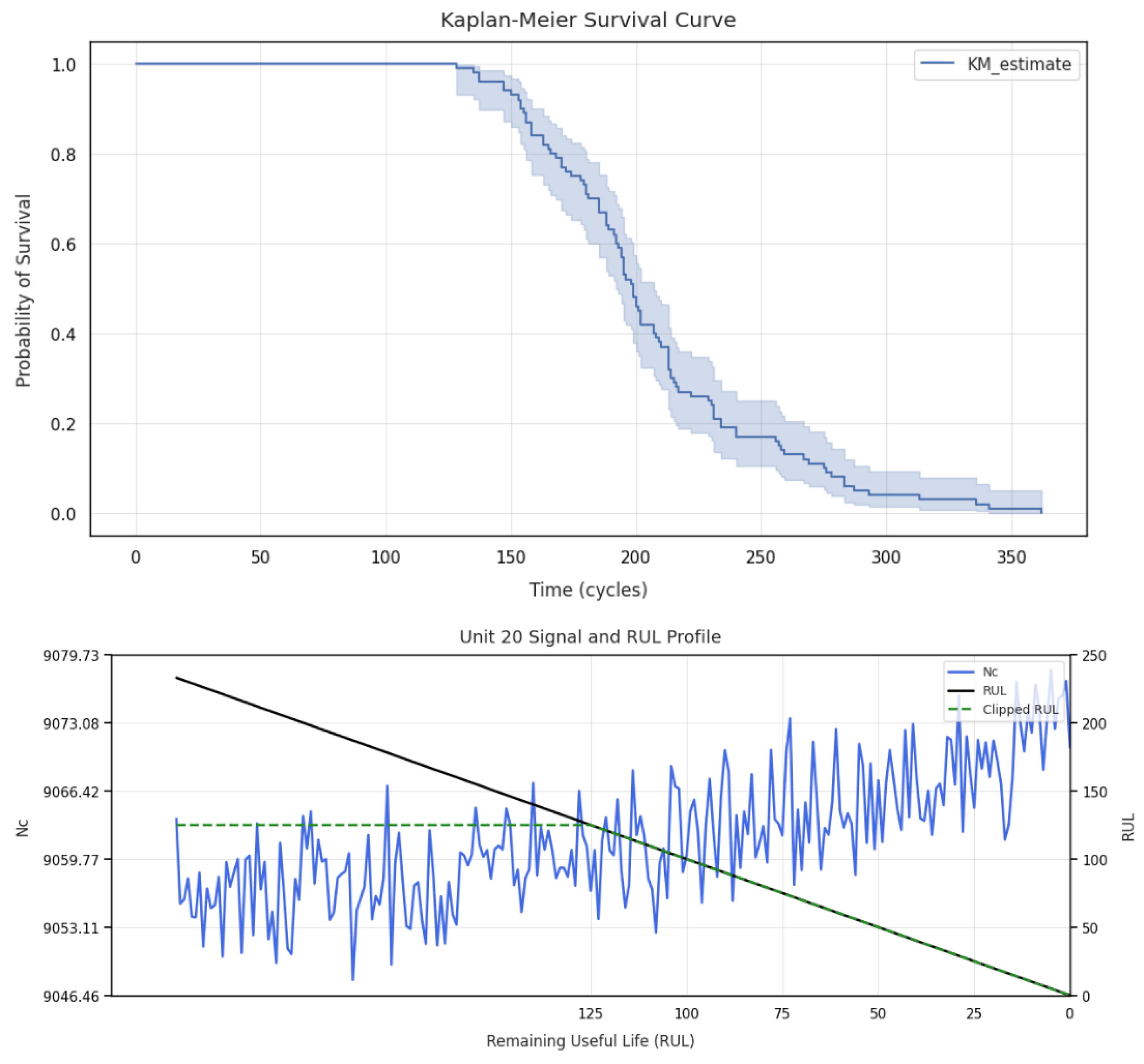
The integration of survival analysis presented in Section 2 allows us to leverage the insights gained from the Kaplan–Meier estimation to establish a more detailed RUL extraction procedure. In contrast, the CMAPSS training dataset collects the machine’s entire lifespan from the operational start to EoL without a clear indication of the RUL, which represents the latent degradation target.

The results from the tailored survival analysis, through Kaplan–Meier estimation curves, define different time (operational cycles) thresholds (for the two different classes of datasets, FD1–FD3 (single operational conditions) and FD2–FD4 (multiple operational condition), when the survival probability starts to decrease, standing at cycle 125 for the first set and cycle 150 for the second set.

Figure 6, which refers to the FD1 dataset, clearly shows how the survival threshold and the sensor drift (Nc sensor) are correlated, thereby giving the possibility of a more refined degradation analysis and RUL extraction, which determines better model training and performance, mitigating pitfalls related to internal parameter modifications in far EoL conditions.

5. Robust Conformal Prognostic for Reliable Predictive  Maintenance

In PdM, accurately forecasting RUL from sensor data is critical for ensuring timely interventions and minimizing downtime. Nonetheless, real-world constraints can lead to nuanced modeling challenges with the target RUL extraction, commonly derived under simplified assumptions such as a piecewise linear degradation model as presented in Section 4, under-representing the actual degradation patterns and especially impairing the performance of probabilistic models.

5.1. Uncertainty Quantification Methodologies in Predictive Maintenance

Bayesian models (e.g., Bayesian Neural Network, Prophet) assume that errors or residuals follow a specified distribution (e.g., normal distribution), and when the underlying degradation process is oversimplified assumptions (e.g., using the piecewise linear model as in Section 4), these models assume and leverage a pattern that does not match the true variability and complexity of the data, delivering inaccurate results when used for test inference.

Figure 7 represents the problem of leveraging the FD2 dataset from the CMAPSS data collection. The prophet algorithm, introduced in Section 3.1, overfits the data distributions and produces statistically coherent “probabilistic gaps” that fail to capture the actual sensor-based dynamics. Overestimating the piecewise linear trend imposed in the RUL extraction phase can make an impractical strategy for real-world applications where degradation does not strictly follow a piecewise linear path.

Conversely, CP, introduced in Section 3.2, provides a more flexible and distribution-free CI adapted to the actual degradation pattern inherent in the data, permitting practitioners to apply a UQ strategy to independently evaluate the modeling and the CI estimation. Despite the advantages of the CP approach for time series analysis, it necessitates regulation for real PdM applications since it does not inherently embed maintenance domain knowledge, such as the physical requirement that RUL must decrease over time. In fact, if not adequately regulated, the conformal intervals can fluctuate in response to short-term sensor noise, causing large, erratic swings in the predicted intervals and making this practice unfeasible for effective maintenance planning. This tension between purely probabilistic modeling and the need for physically coherent forecasts highlights the motivation for a robust CP framework that regulates prediction and the CI intervals, supporting a rational application to IoT-enabled PdM.

This methodology is the most embodied core of this work. Firstly, it enforces the monotonicity in the predicted RUL sequence (e.g., preventing any non-decreasing segments), which aligns with the real-world nature of degradation processes. After that, to refine the conformal intervals by comparing multiple margin estimators, such as naive quantile, exponential weighting, or bootstrap—and selecting the methodology with the largest coverage. This methodological application ensures that while the coverage guarantees of CP are maintained, it will strengthen predictive margins through a conservative approach. The final intervals remain physically plausible, respecting the PdM practice. Practically, this regulated CP strategy is found especially valuable for PdM decision-making, as it yields intervals that are both statistically valid. To reflect the true component wear while permitting optimized scheduled interventions aiming to preserve the estimation confidence through a more refined CI. Leveraging this tool, a maintenance engineer can combine domain knowledge and a data-driven approach. Looking at both RUL prediction and interval estimation and applying maintenance strategies that reduce unexpected failures to optimize resource allocation and productivity in industrial environments.

5.2. Robust Conformal Prognostic Design

The proposed prognostic workflow, presented in Figure 8, begins by generating RUL estimations from prognostic algorithms. To compare the validation performances, these initial predictions passed through a regulation step where non-increasing monotonicity is enforced to ensure that RUL does not inappropriately increase over time. This represents a critical constraint in most degradation processes.

Next, the framework proceeds to the calibration and residuals phase, where the regulated predictions are compared against true values from a calibration set (training set) to compute residuals, and the margin estimators are applied to these residuals to quantify the uncertainty. Specifically, this work considers the three main strategies introduced in Section 3.2 (naive, bootstrapping, weighted margin), which are commonly applied in time series conformal applications:

• Naive margin (Quantile 1$-\alpha$) uses a straightforward quantile-based approach.
• Bootstrap margin (median bootstrap) leverages resampling to obtain robust estimates of variability.
• Weighted margin (exponential weighting) accounts for time-varying or instance-specific importance.

The latter phase consists of comparing or combining the calculated margin with the final confidence. To further halve (without considering a superior CI) and conservatively adjust to avoid excessively wide intervals (selecting the appropriate confidence value $\alpha$), reflecting engineering judgment and domain requirements for safety and cost considerations. Given these conditions, the outlined approach constructs the final prediction interval, intentionally bounded above by the regulated prediction. It preserves the strictly decreasing RUL trajectory and mitigates undue sensitivity to sensor noise. The CI estimation provides coverage that aligns with the desired confidence levels. It gives the possibility to evaluate the proximity to the EoL score, which gives an idea of the model’s conservativeness by calculating the time window distance between the conformal critical status (when CI predicts RUL = 0) and the actual EoL (when validation RUL = 0) to allow engineers and practitioners to evaluate whether immediate intervention is warranted or if further analysis is possible before triggering timely interventions.

Overall, this end-to-end pipeline offers a coherent, physically plausible, and statistically reliable combination of conformal calibration and decision-oriented. The proposed forecasting framework avoids common pitfalls related to probabilistic methods (which may overfit idealized trends) and unregulated conformal approaches (which can be unduly influenced by sensor noise). This delivers robust intervals that expand the timely estimation of RUL, streamline maintenance scheduling, and ultimately improve the reliability and cost-effectiveness of PdM programs.

5.3. Experimental Setting

This section aims to present the background and experimental settings of the aforementioned prognostic workflow, introduced in Section 5.2. It offers a coherent strategy to evaluate different algorithms and select the best learning approach. To inherently better capture the patterns between the data and the RUL, it compares the different CI estimation approaches.

In PdM, the same types of equipment or ensembles of assets can operate under different conditions and noise levels, generating simple or more complex degradation patterns. This peculiarity highlights the need for a rigorous selection of a learning strategy supported by extensive experimentation. The CMAPSS dataset, introduced in Section 4, represents a well-known case study in PdM. It will be used within this experimentation, utilizing a unit-wise train validation splitting as 80% for training and 20% for validation, with a context window for batch and lag generation set to 30 lags (which is a standard size for DL strategies).

5.3.1. Algorithm Selection and Rationale

Critical for the algorithm selection and subsequent hyperparameter selection are the data characteristics and the relative predictive maintenance problem:

• High-dimensional multi-rate sensor streams: each turbofan in CMAPSS produces 21–24 heterogeneous channels whose interactions are highly non-linear [21].
• Regime switches and concept drift: the sensors’ drift effects violate the covariance-stationarity required by autoregressive and statistical models.
• Piece-wise-linear RUL target: RUL is not directly observed but constructed ex-post from survival information;

Following the characteristics of the predictive maintenance problem, learning mechanisms selected for this evaluation span from DL architectures, including LSTM, BiLSTM, NBEATS, and a hybrid CNN-GRU architecture, to ML techniques and XGBoost regressor, serving to benchmark simple and more advanced strategies through different learning mechanisms. An overview of the selected hyperparameters for each model is presented in

Table 2. Hyperparameter setting of the implemented models.

Model	Hyperparameters
LSTM	3 LSTM layers with 300, 250, and 200 units (tanh activation)
	Dropout rate: 0.5 after each LSTM layer
	Batch Normalization after each LSTM layer
	Dense layer with 100 neurons (ReLU) and final single output neuron
	Optimizer: Adam, Learning rate: 0.0005
	Batch size: 32, Epochs: configurable (50–100)
BiLSTM	Same hyperparameters of LSTM but with BiLSTM layers
NBEATS	2 Fully connected dense blocks
	Each block: 2 dense layers with 256 neurons (ReLU activation)
	Optimizer: Adam, Learning rate: 0.001
CNN-GRU	1D Convolutional layer: 64 filters, kernel size 3 (ReLU)
	GRU layer with 100 units
	Dense layers: 50 neurons followed by a single-neuron output
	Optimizer: Adam, Learning rate: 0.001
XGBoost	Maximum tree depth: 60
	Learning rate: 0.01, Number of estimators: 200
	Subsample ratio: 0.8, Colsample ratio: 0.8

.

5.3.2. Performance Metrics and Evaluation Procedure

Model performances have been properly evaluated using several metrics, including Mean Squared Error (MSE), Mean Absolute Error (MAE), Root Mean Squared Error (RMSE), and the Coefficient of Determination ($R^2$). In addition, a custom S-score, given by Saxena et al. [21], is employed to evaluate prognostic performance by asymmetrically penalizing over-estimations and under-estimations. More precisely, the S-score, defined as in Equation (21), is chosen as the principal metric for model selection since its straightforward impact in PdM practices is due to its weighted approach near EoL.

$$S=\sum _i\left\{\begin{array}{cc}exp\left(-{\displaystyle \frac{{\mathrm{rul}}_{\mathrm{pred},i}-{\mathrm{rul}}_{\mathrm{true},i}}{13}}\right)-1,\hfill & \mathrm{if}{\mathrm{rul}}_{\mathrm{pred},i}<{\mathrm{rul}}_{\mathrm{true},i},\hfill \\ exp\left({\displaystyle \frac{{\mathrm{rul}}_{\mathrm{pred},i}-{\mathrm{rul}}_{\mathrm{true},i}}{10}}\right)-1,\hfill & \mathrm{otherwise}.\hfill \end{array}\right.$$

(21)

5.3.3. Uncertainty-Quantification Techniques

To complement punctual predictions with reliable uncertainty estimates, CP intervals are computed, with the selected hyperparameters of these conformal strategies listed in

Table 3. Conformal methods and their key hyperparameters.

Method	Hyperparameters
Naive Margin	$\alpha =0.05$; Margin = $(1-\alpha )$
Weighted Exponential Margin	$\alpha =0.05$; Weights: $w_i=exp\left({\displaystyle \frac{i}{n/5}}\right)$
Bootstrap Margin	$\alpha =0.05$; $B=200$ bootstrap samples;

.

Concerning the CI estimation, the benchmarking of different CP strategy methodologies is implemented using the calibration set for the entire training set and then computing the coverage as the fraction of calibration samples, as presented in Equation (19). The CP pipeline internally selects the margins that achieve the highest coverage on the calibration set. It ensures that the chosen CI meets the desired coverage level while effectively balancing the width of the prediction intervals and the predictive performance and chooses the best strategic approach. Among the aforementioned triplet, analyze and adopt the CP procedure, which provides the overall highest coverage. Additionally, to understand the conservativeness of the CP, the proximity to the EoL score is calculated using the validation sets as the distances between the conformal and actual EoL for each unit, with a smaller value of ${\Delta }_{\mathrm{index}}$ indicating that the predicted interval captures the timing of the EoL closely, while a larger value suggests a misalignment between the predicted and actual events. In conclusion, the proposed experimental pipeline, applied across the CMAPSS datasets, aims to facilitate a comprehensive comparison between advanced DL architectures and classical ML methods for RUL prediction while giving a solid framework to evaluate different conformal strategy integrations.

6. Experimental Results and Performance Evaluation: A Case Study on CMAPSS Datasets

To evaluate the effectiveness of the proposed Robust Conformal Prognostic methodology, different experiments on the four CMAPSS datasets have been conducted, referring to the workflow of Section 4 and adopting the design and performance evaluation settings of Section 5.3.

In particular, the FD2 dataset is fully evaluated in Section 6.1, as it represents a complex and realistic scenario with high operational variability, ensuring a comprehensive assessment of the proposed approach and allowing for a qualitative benchmark against previous methodologies such as Conformal Prediction and probabilistic confidence estimation, whose results are presented in Section 5. Conversely, the aggregated results for the other datasets are provided in Section 6.1, serving as supplementary validation to support the overall findings. Specifically, LSTM and BiLSTM exhibit particularly steady convergence, likely reflecting their capacity to capture long-range temporal dependencies in the sensor data, while N-BEATS experiences a rapid initial descent but then plateaus at relatively higher loss values, highlighting its modest capabilities when applied in a complex data environment.

6.1. Detailed Performance Analysis on FD004

A broader perspective on the training process can be obtained by examining the aggregated loss curves, as presented in Figure 9.

The hybrid architecture CNN-GRU surpasses the other metrics in terms of training loss by continuing to decline smoothly, effectively handling the noisy pattern in the sensor through its convolutional masks acting as a feature engineering layer and managing the slight non-stationarity in degradation trajectories.

Moving to the final predictive performance, Figure 10 compares the S-score, MAE, RMSE, and $R^2$ for LSTM, BiLSTM, N-BEATS, CNN-GRU, and XGBoost. These lower performances despite DL approaches are possibly due to the combination of its simpler learning approach and the large number of features coming from the preprocessing stage, presented in Section 2, which limits its overall capabilities. In detail, the BiLSTM achieves consistently low MAE and RMSE, reflecting its stability and accuracy in modeling sensor-driven degradation signals. CNNGRU demonstrates resilience to outliers, as evidenced by its favorable S-score. Thus, both appear to be strong choices in this particular PdM scenario.

Moving to the uncertainty scores assessment, the results regarding the calibration metrics are presented in

Table 4. Naive, weighted, and bootstrap conformal methods evaluation using FD2.

Method	Margin	Coverage
Naive	32.92	0.476
Weighted	40.57	0.510
Bootstrap	41.66	0.513

. The conformal scores highlight that the bootstrap approach attains coverage probabilities closest to the desired ($1-\alpha$) while retaining moderate interval widths, indicating a practical compromise between excessive conservatism and insufficient coverage, with bootstrap showing similar reliability but producing marginally broader intervals. These findings underscore the advantages of the bootstrapping conformal strategy in balancing interval tightness with robust coverage, which refines the naive’s ability to adapt to a noisy environment.

The further analysis conducted analyzing the CP metrics on the validation set, presented in Figure 11, shows a coverage distribution that spans from near 0.0 to 1.0, with a moderate median value that is particularly noteworthy given a uniform margin selection approach yielding moderate overall performance. Similarly, the EoL Proximity distribution also presents a moderate alignment between predicted and actual EoL indices, with a subset showing considerable deviations collectively showing that even without strict unit-wise calibration, the model attains reasonably moderate metrics.

6.2. Visual Analysis of Conformal Prediction Intervals

In order to provide an insightful and practical visualization of a single engine unit, Figure 12 offers a detailed view of how weighted calibration performs at $\alpha =0.05$. The orange curve signifies the clamp-regulated RUL prediction, while the green-shaded region indicates the conformal lower bound. Thanks to weighted tendency, which refers to an estimator that tracks recent residuals more closely. The interval is sufficiently tight to convey meaningful uncertainty estimates but remains broad enough to encapsulate abrupt changes in degradation levels.

This flexibility surpasses that of purely probabilistic bounds or naive row-based conformal intervals, which may fail to adapt when sensor signals shift dramatically. Figure 13, on the other hand, expands the analysis to multiple engine units, each concatenated on the x-axis.

Every colored block corresponds to a separate unit’s non-increasing RUL forecast and weighted-based CI. Units with higher starting RULs display narrower CIs that grow gradually, whereas those nearing their EoL reveal broader intervals early on, capturing the heightened sensor volatility. The uniform behavior across units reinforces weighted’s capability to deliver consistent, scenario-adaptive intervals that balance coverage and interval tightness to reduce variability in PdM.

6.3. Aggregate Performance Evaluation

Table 5. Combined Metrics Evaluation of CMAPSS datasets: predictive and UQ algorithms.

Metric	FD1	FD2	FD3	FD4
Model Metrics
Model	NBEATS	CNN-GRU	NBEATS	BiLSTM
MSE	347.67	300.32	226.29	505.239090
MAE	14.34	13.06	10.610778	17.281365
RMSE	18.64	17.73	15.04	22.477524
R2	0.86	0.82	0.911	0.800323
S-score	24069	75307	22870	273456
Conformal Metrics
Method	Weighted	Bootstrap	Weighted	Weighted
Coverage	0.505	0.513	0.423	0.488
Margin	40.171	41.63	36.06	64.52

presents a comprehensive view of both the point estimate metrics and the conformal metrics across all four FD subsets. These results highlight the variability in model accuracy under different operating conditions and fault modes while also illustrating the effectiveness of conformal calibration in quantifying predictive uncertainty. The highest $R^2$ values and the lowest error metrics (MSE, MAE, RMSE) for the FD1–FD3 dataset class are achieved using the N-BEATS model, suggesting that the chosen architectures can capture sensor behavior more effectively when fewer operating regimes and clearly defined fault modes are involved. Conversely, FD4 poses the most significant challenge due to its complexity and broader operational variability, as evidenced by higher S-scores and slightly inflated error metrics, proposing more complex architectures as the best option for the RUL estimation.

The CP patterns are consistent with Section 3, where the weighted approach proved more adaptive by assigning larger weights to recent residuals in exchangeable conditions, whereas bootstrap instead seems to be more suitable for datasets with slight drifts and a noticeable amount of noise. The metrics underline the difficulty of maintaining highly precise uncertainty intervals in non-stationary environments, with the robust conformal framework helping to keep deviations within a useful range for practical maintenance actions.

7. Discussion

The extensive experimentation described in Section 6 illustrates the practical value of the Robust Conformal Prognostic framework when applied to the CMAPSS dataset. Models such as CNN-GRU and BiLSTM consistently demonstrate superior performance, particularly in the FD4–FD2 datasets (see Section 4), suggesting that their capacity to capture both temporal dependencies and localized signal variations is instrumental in handling complex operational regimes. However, NBEATS’ present performance plateaus at a higher error level, capturing abrupt shifts in sensor readings may require additional architectural modifications or domain-specific regularizations, especially in more complex scenarios (FD2–FD4). In particular, the weighted margin approach, discussed in Section 3.2, demonstrates the most stable coverage performance across a range of scenarios; in fact, by emphasizing recent residuals, it adeptly adjusts interval widths whenever sensor data exhibit sudden changes, presenting sufficiently tight CI while also remaining flexible enough to encompass unexpected degradation trajectories. Generally, By coupling deep-learning prognostics with distribution-free, clamp-regulated Conformal Prediction, the proposed framework does more than improve accuracy; it operationalizes machine trustworthiness in streaming environments. The resulting pair—RUL point estimate and validated lower-bound—constitutes an intelligence signal upstream that IoT platforms can readily consume. In a fully AI-enabled stack, this signal becomes a catalyst for closed-loop autonomy: edge gateways can down- or up-sample sensors according to risk, cloud-based optimizers can resequence production or logistics, and digital-twin layers can run “what-if” scenarios driven by calibrated failure horizons. Because the interval is guaranteed valid irrespective of data drift or regime shifts, it provides a robust decision substrate across heterogeneous devices, locations, and update cycles, extending its value beyond the single-asset case.

8. Conclusions

In conclusion, the Regulated Conformal Prognostic framework presented in this paper provides a comprehensive and adaptable approach to PdM under diverse operating conditions and fault modes. By synthesizing DL architectures, conformal theory, and domain-specific constraints, it ensures that RUL estimates are both statistically well-calibrated and physically coherent. The methodology effectively balances accuracy and interval tightness while maintaining desirable coverage properties, ensuring that maintenance planners can rely on the intervals produced without incurring excessive conservatism. The experimental evidence supports the notion that monotonic regulation appreciably enhances the practical utility of RUL forecasts. Specifically, enforcing strictly non-increasing trajectories aligns with real-world degradation processes, mitigating the detrimental effects of sensor noise and abrupt operational shifts. Moreover, the weighted margin estimator stands out for its ability to adapt to local trends in the residual distribution, thereby delivering a compelling blend of coverage stability and predictive adaptability. Overall, the results attest to the efficacy of combining DL architectures and conformal calibration for high-fidelity prognostics, offering clear pathways for integration into industrial PdM workflows. Future research could extend this framework by exploring additional domain constraints, applying more advanced learning strategies to adapt the models across equipment types, or incorporating data augmentation strategies to handle data-scarce regimes. In doing so, the outlined Conformal Prognostic methodology can become an even more versatile and powerful tool for advancing reliability, cost-effectiveness, and safety in complex engineering systems.

References

1. Bonomi, F.; Milito, R.; Natarajan, P.; Zhu, J. Big data and internet of things: A roadmap for smart environments. Stud. Comput. Intell. 2014, 546, 169–186. [Google Scholar]
2. Killeen, P.; Parvizimosaed, A. An AHP-Based Evaluation of Real-Time Stream Processing Technologies in IoT; Course report; Faculty of Engineering, University of Ottawa: Ottawa, ON, Canada, 2018. [Google Scholar]
3. Mobley, R. An Introduction to Predictive Maintenance; Butterworth-Heinemann: Oxford, UK, 2002. [Google Scholar] [CrossRef]
4. Zhang, W.; Yang, D.; Wang, H. Data-Driven Methods for Predictive Maintenance of Industrial Equipment: A Survey. IEEE Syst. J. 2019, 13, 2213–2227. [Google Scholar] [CrossRef]
5. Sirvio, K. Intelligent Systems in Maintenance Planning and Management. Intell. Syst. Ref. Libr. 2015, 87, 221–245. [Google Scholar] [CrossRef]
6. Den Hartog, J. Mechanical Vibrations; Courier Corporation: North Chelmsford, MA, USA, 2008. [Google Scholar]
7. Jardine, A.; Lin, D.; Banjevic, D. A review on machinery diagnostics and prognostics implementing condition-based maintenance. Mech. Syst. Signal Process. 2006, 20, 1483–1510. [Google Scholar] [CrossRef]
8. Fernandes, M.; Canito, A.; Bolón-Canedo, V.; Conceição, L.; Praça, I.; Marreiros, G. Data analysis and feature selection for predictive maintenance: A case-study in the metallurgic industry. Int. J. Inf. Manag. 2019, 46, 252–262. [Google Scholar] [CrossRef]
9. Zhou, H.; Huang, X.; Wen, G.; Lei, Z.; Dong, S.; Zhang, P.; Chen, X. Construction of health indicators for condition monitoring of rotating machinery: A review of the research. Expert Syst. Appl. 2022, 203, 117297. [Google Scholar] [CrossRef]
10. Saidy, C.; Xia, K.; Kircaliali, A.; Harik, R.; Bayoumi, A. The Application of Statistical Quality Control Methods in Predictive Maintenance 4.0: An Unconventional Use of Statistical Process Control (SPC) Charts in Health Monitoring and Predictive Analytics; Springer: Cham, Switzerland, 2020; pp. 1051–1061. [Google Scholar] [CrossRef]
11. Cai, Y.; Teunter, R.H.; de Jonge, B. A data-driven approach for condition-based maintenance optimization. Eur. J. Oper. Res. 2023, 311, 730–738. [Google Scholar] [CrossRef]
12. Christou, I.T.; Kefalakis, N.; Zalonis, A.; Soldatos, J.; Bröchler, R. End-to-End Industrial IoT Platform for Actionable Predictive Maintenance. IFAC-PapersOnLine 2020, 53, 173–178. [Google Scholar] [CrossRef]
13. Paolanti, M.; Romeo, L.; Felicetti, A.; Mancini, A.; Frontoni, E.; Loncarski, J. Machine Learning Approaches for Predictive Maintenance. In Proceedings of the 2018 14th IEEE/ASME International Conference on Mechatronic and Embedded Systems and Applications (MESA), Oulu, Finland, 2–4 July 2018. [Google Scholar]
14. Kumar, S.; Raj, K.K.; Cirrincione, M.; Cirrincione, G.; Franzitta, V.; Kumar, R.R. A Comprehensive Review of Remaining Useful Life Estimation Approaches for Rotating Machinery. Energies 2024, 17, 5538. [Google Scholar] [CrossRef]
15. Bhatnagar, A.; Wang, H.; Xiong, C.; Bai, Y. Improved Online Conformal Prediction via Strongly Adaptive Online Learning. arXiv 2023, arXiv:2302.07869. [Google Scholar] [CrossRef]
16. Chen, T.; Guestrin, C. XGBoost: A Scalable Tree Boosting System. In Proceedings of the 22nd ACM SIGKDD International Conference on Knowledge Discovery and Data Mining, San Francisco, CA, USA, 13–17 August 2016; pp. 785–794. [Google Scholar] [CrossRef]
17. Yousuf, S.; Khan, S.A.; Khursheed, S. Remaining Useful Life (RUL) Regression Using Long–Short Term Memory (LSTM) Networks. Microelectron. Reliab. 2022, 139, 114772. [Google Scholar] [CrossRef]
18. Guo, X.; Wang, K.; Yao, S.; Fu, G.; Ning, Y. RUL Prediction of Lithium Ion Battery Based on CEEMDAN-CNN BiLSTM Model. Energy Rep. 2023, 9, 1299–1306. [Google Scholar] [CrossRef]
19. Oreshkin, B.N.; Carpov, D.; Chapados, N.; Bengio, Y. N-BEATS: Neural Basis Expansion Analysis for Interpretable Time Series Forecasting. arXiv 2019, arXiv:1905.10437. [Google Scholar]
20. Azyus, A.F.; Wijaya, S.K.; Naved, M. Prediction of Remaining Useful Life Using the CNN-GRU Network: A Study on Maintenance Management. Softw. Impacts 2023, 17, 100535. [Google Scholar] [CrossRef]
21. Saxena, A.; Goebel, K.; Simon, D.; Eklund, N. Damage propagation modeling for aircraft engine run-to-failure simulation. In Proceedings of the 2008 International Conference on Prognostics and Health Management, Denver, CO, USA, 6–9 October 2008. [Google Scholar] [CrossRef]
22. Fink, O.; Wang, Q.; Svensen, M.; Dersin, P.; Lee, W.J.; Ducoffe, M. Potential, challenges and future directions for deep learning in prognostics and health management applications. Eng. Appl. Artif. Intell. 2020, 92, 103678. [Google Scholar] [CrossRef]
23. Tiddens, W.; Braaksma, A.; Tinga, T. The Adoption of Prognostic Technologies in Maintenance Decision Making: A Multiple Case Study. Procedia CIRP 2015, 38, 171–176. [Google Scholar] [CrossRef]
24. Lei, Y.; Li, N.; Guo, L.; Li, N.; Yan, T.; Lin, J. Machinery health prognostics: A systematic review from data acquisition to RUL prediction. Mech. Syst. Signal Process. 2018, 104, 799–834. [Google Scholar] [CrossRef]
25. Roemer, M.; Byington, C.; Kacprzynski, G.; Vachtsevanos, G.; Goebel, K. Prognostics. In Systems Health Management with Aerospace Applications; Johnson, S., Gormley, T., Kessler, S., Mott, C., Patterson-Hine, A., Reichard, K., Scandura, P., Jr., Eds.; John Wiley & Sons, Ltd.: Hoboken, NJ, USA, 2011; pp. 281–295. [Google Scholar]
26. Vachtsevanos, G.; Goebel, K. Basic principles. In Integrated Vehicle Health Management: Perspectives on an Emerging Field; Jennions, I., Ed.; SAE International: Warrendale, PA, USA, 2011; pp. 55–66. [Google Scholar]
27. Goebel, K.; Vachtsevanos, G. Algorithms and their impact on integrated vehicle health management. In Integrated Vehicle Health Management: Perspectives on an Emerging Field; Jennions, I., Ed.; SAE International: Warrendale, PA, USA, 2011; pp. 67–76. [Google Scholar]
28. Simundic, A.M. Confidence interval. Biochem. Medica 2008, 18, 154–161. [Google Scholar] [CrossRef]
29. Microsoft. Automate Model Training with the ML.NET CLI—ML.NET. 2024. Available online: https://learn.microsoft.com/en-us/dotnet/machine-learning/automate-training-with-cli (accessed on 25 March 2025).
30. Hyndman, R.J.; Athanasopoulos, G. Forecasting: Principles and Practice. OTexts. 2021. Available online: https://otexts.com/fpp3/ (accessed on 25 March 2025).
31. Žunić, E.; Korjenić, K.; Hodžić, K.; Đonko, D. Application of Facebook’s Prophet Algorithm for Successful Sales Forecasting Based on Real-World Data. Int. J. Comput. Sci. Inf. Technol. (IJCSIT) 2020, 12, 23–36. [Google Scholar] [CrossRef]
32. Manokhin, V. Practical Guide to Applied Conformal Prediction in Python: Learn and Apply the Best Uncertainty Frameworks to Your Industry Applications; Packt Publishing Ltd.: Birmingham, UK, 2023. [Google Scholar]
33. Qian, W.; Zhao, C.; Li, Y.; Ma, F.; Zhang, C.; Huai, M. Towards Modeling Uncertainties of Self-explaining Neural Networks via Conformal Prediction. arXiv 2024, arXiv:2401.01549. [Google Scholar] [CrossRef]
34. Guo, C.; Pleiss, G.; Sun, Y.; Weinberger, K.Q. On Calibration of Modern Neural Networks. arXiv 2020, arXiv:2109.12156. [Google Scholar]
35. Barber, R.F.; Candès, E.J.; Ramdas, A.; Tibshirani, R.J. Conformal Prediction Beyond Exchangeability. arXiv 2022, arXiv:2202.13415. [Google Scholar] [CrossRef]
36. Arias Chao, M.; Kulkarni, C.; Goebel, K.; Fink, O. Aircraft Engine Run-to-Failure Dataset under Real Flight Conditions for Prognostics and Diagnostics. Data 2021, 6, 5. [Google Scholar] [CrossRef]
Figure 1. Graphical Overview of the robust IoT-enabled PdM framework.
Futureinternet 17 00244 g001
Figure 2. Data workflow in real-time IoT environment: sensors, ingestion, and data processing.
Futureinternet 17 00244 g002
Figure 3. Visualization of a typical turbofan degradation pattern.
Futureinternet 17 00244 g003
Figure 4. Turbofan Engine System, Saxena et al. [21].
Futureinternet 17 00244 g004
Figure 5. Exploratory data analysis of FD1–FD2: each color representing a different machine ID.
Futureinternet 17 00244 g005
Figure 6. Survival analysis, Linear RUL, and early RUL extraction for FD1.
Futureinternet 17 00244 g006
Figure 7. Example of UQ methodology using Unit 260 of CMAPSS: Probabilistic Model (Prophet) and Conformal Predictions via BiLSTM.
Futureinternet 17 00244 g007
Figure 8. Regulated Conformal Prognostic Design.
Futureinternet 17 00244 g008
Figure 9. Aggregated FD2 loss curves for LSTM, BiLSTM, N-BEATS, and CNN-GRU, illustrating differences in convergence behaviors.
Futureinternet 17 00244 g009
Figure 10. Final FD2 performance metrics for LSTM, BiLSTM, NBEATS, CNN-GRU, and XGBoost.
Futureinternet 17 00244 g010
Figure 11. Weighted CP performance evaluation in FD2 validation set.
Futureinternet 17 00244 g011
Figure 12. Single-unit conformal interval for unit 43 with weighted calibration at α = 0.05 , illustrating a stable yet adaptive lower bound.
Futureinternet 17 00244 g012
Figure 13. Multi-unit conformal intervals aligned on the x-axis, with each segment depicting clamp-regulated predictions and weighted-based bounds for a distinct engine unit.
Futureinternet 17 00244 g013