Article

Explainable Artificial Intelligence Approach for Improving Head-Mounted Fault Display Systems

IMT Nord Europe, Center for Digital Systems, University of Lille, F-59000 Lille, France
*
Author to whom correspondence should be addressed.
These authors contributed equally to this work.
Future Internet 2024, 16(8), 282; https://doi.org/10.3390/fi16080282
Submission received: 3 July 2024 / Revised: 29 July 2024 / Accepted: 31 July 2024 / Published: 6 August 2024
(This article belongs to the Special Issue Artificial Intelligence-Enabled Internet of Things (IoT))

Abstract

:
To fully harness the potential of wind turbine systems and meet high power demands while maintaining top-notch power quality, wind farm managers run their systems 24 h a day/7 days a week. However, due to the system’s large size and the complex interactions of its many components operating at high power, frequent critical failures occur. As a result, it has become increasingly important to implement predictive maintenance to ensure the continued performance of these systems. This paper introduces an innovative approach to developing a head-mounted fault display system that integrates predictive capabilities, including deep learning long short-term memory neural networks model integration, with anomaly explanations for efficient predictive maintenance tasks. Then, a 3D virtual model, created from sampled and recorded data coupled with the deep neural diagnoser model, is designed. To generate a transparent and understandable explanation of the anomaly, we propose a novel methodology to identify a possible subset of characteristic variables for accurately describing the behavior of a group of components. Depending on the presence and risk level of an anomaly, the parameter concerned is displayed in a piece of specific information. The system then provides human operators with quick, accurate insights into anomalies and their potential causes, enabling them to take appropriate action. By applying this methodology to a wind farm dataset provided by Energias De Portugal, we aim to support maintenance managers in making informed decisions about inspection, replacement, and repair tasks.

1. Introduction

Artificial intelligence has catalyzed significant changes, propelling more companies into the Industry 4.0 and 5.0 eras. Recently, numerous machine learning-based tools have been developed and deployed across various industrial applications. These tools utilize data-driven analytical methods to predict and diagnose system health during operations [1,2]. In the energy sector, particularly within wind energy systems, these approaches provide numerous competitive advantages, including reduced maintenance costs and enhanced system efficiency and reliability [3].
More precisely for predictive maintenance (PdM) purposes, numerous techniques have been developed and refined in recent years for anomaly detection [4]. For this, several methodologies based on supervised learning can be examined, including multilayer perceptron (MLP) [5] and manifold learning [6,7]. Additionally, unsupervised methods, such as DBSCAN—a density-based clustering algorithm—have proven effective in identifying anomalous data [8]. Throughout this research, AI has shown significant promise and capability in addressing fault detection problems. Notably, studies such as [9,10] have highlighted the effectiveness of the LSTM model in capturing long-term dependencies by selectively updating and retrieving information, thus integrating past behavior into the diagnostic model to predict future conditions (normal or abnormal). However, for maintenance to be genuinely effective, greater emphasis must be placed on fault management. Simply enhancing the maintenance program is insufficient for today’s advanced physical systems.
In this context, one approach is to equip the supervision system with a mechanism for interpreting the encountered problems. The main challenge is to detect the occurrence of an anomaly and provide a plausible cause or explanation, allowing human operators to determine the appropriate response quickly [11]. This is where explainable artificial intelligence (XAI) becomes valuable, promoting a shift towards contextual, human-centered, understandable, and reliable explanations [12]. Initially, Explainable AI (XAI) concentrated on developing methods to make black-box models more understandable, like deep neural networks. This encompasses a range of model-agnostic techniques such as Anchor [13], LIME [14], LORE [15], LUX [16], and SHAP [17]. Additionally, there are model-specific approaches that utilize gradient-based deviations from the reconstruction of input features [18] or the internal features of particular machine learning algorithms. An example is GradCam [19], specifically designed for deep neural networks. Alongside these research works, another emerging trend emphasizes the development of efficient glass-box models [20], which are inherently interpretable. Examples include explainable boosting machines [21] and, more recently, prototype deep neural networks. Regardless of the underlying techniques the XAI methods aim to explain the model’s decisions by describing the relationship between the model input and output. This description can be presented in various forms [22], such as feature importance, feature impact, decision rules, prototypes, and examples. Providing these explanations builds end-user trust in the model and enhances understanding, which can be used to model debugging, data debiasing, etc., contributing to boosting the model performance.
In this paper, we propose enhancing transparency, confidence, and intelligibility in decision automation systems by leveraging the interpretability of AI models. In other words, the paper introduces a methodology to design a head-mounted fault display system that combines predictive capabilities (through deep learning model integration) with anomaly explanations (focusing on model transparency and comprehensibility) to enhance predictive maintenance tasks. In essence, it presents a methodology to design an efficient system that interactively presents identified faults through an explicative Head Mounted Fault Display (xHMFD) system. This system is developed from sampled and recorded data generated by the physical system and data generated by a deep neural diagnoser model. The integrated solution will go beyond detecting the required anomaly. As such, it will also provide insight into the unusual behavior of the wind turbine for each component, as well as their criticality. This allows the maintenance manager to optimally adapt their maintenance program to the observed anomaly.
However, it is important to note that over the past few decades, head-mounted display systems have been extensively utilized to monitor complex systems, demonstrating their effectiveness [23,24]. Alves et al. [25] extended the use of these systems beyond monitoring to support maintenance tasks. In their approach, videos, images, and 3D animations assist technicians during maintenance operations, enabling less specialized personnel to perform these tasks. While these applications are effective, augmented reality (AR) may not always be suitable, as it requires technicians to physically travel to wind farms, which can be both costly and time-consuming. To address this issue, some research has explored using mixed reality (MR) for remote maintenance [26]. In this approach, the maintenance manager uses an augmented reality device to display instructions, while the technician receives the manager’s view on their computer. This highlights the limited adoption of virtual reality (VR) among researchers, primarily due to the need for the physical maintenance and visual assessment of machinery.
Our paper addresses this challenge by proposing the integration of a 3D model created from sampled and recorded data with a deep neural diagnoser model. This innovative approach aims to identify and locate anomalies in the head-mounted fault display system using virtual reality, but it also provides tangible explanations to maintenance operators to facilitate their tasks. As a proof of concept, we apply the methodology to a wind farm dataset provided by EDP (Energias De Portugal) company. Feasibility and performance are discussed in this paper.

2. Explicative Head-Mounted Fault Display System Design

This section outlines the design of an explicative head-mounted fault display system using virtual reality. This system integrates predictive capabilities via deep learning models with anomaly explanations, focusing on transparency and comprehensibility to improve predictive maintenance tasks. However, designing a head-mounted fault display system using VR involves several key steps, each integrating hardware and software components to ensure an effective and user-friendly system. In other terms, the primary goal is to design an effective head-mounted fault display system using virtual reality that enhances fault detection, localization, and explanation, and predictive maintenance capabilities, improving operational efficiency and providing a more immersive and informative user experience, particularly in the case of wind turbine maintenance. Below are the main steps to guide the design process.

2.1. System Architecture

The solution follows the architecture illustrated in Figure 1 designed to function on a VR headset as well as on a computer, guaranteeing that the user can access the application even in the case that no functional headset is available. In other terms, the application works similarly on the computer and the xHMFD system versions, the only difference being the movement and interaction controls.
As illustrated in Figure 1, the system is divided into three components: (i) the failure diagnoser server and model, and (ii) the Unity server, part of the system core, for overall implementation. A robust computer system capable of handling VR applications and real-time data processing is particularly selected in this case to support the application. (iii) The last part is the clients using the application. One selects a VR headset that offers high resolution, comfortable wear, and reliable tracking. The interaction between the different parts is as follows. First, the failure diagnoser model receives data from the wind turbines via the Unity server and uses the deep learning model to predict potential issues. Second, the Unity server acts as the core of the application, storing all turbine information, which it then passes on to the various clients and the anomaly diagnoser server. Finally, the clients are the application instances running on virtual reality devices, displaying the wind farm and the associated data collected via the application running on the computer. Let us notice that sensor data from the turbines are sent to the Unity server, which serves as a mediator between the clients and the anomaly detection server. When the server receives new data, it updates the clients with the latest information. Additionally, it sends the data to the fault diagnoser server, which predicts the current state of the turbines and compares it with the actual status. Any identified anomalies are reported to the Unity server, allowing the computer application to visualize them and provide this information to clients for further action.

2.2. User Interface Design

The user interface should be designed with a human-centered approach to encourage the maintenance operators to interact with computers in an intuitive, human-like manner. Then, the main objective is to create an enjoyable experience for both novice and expert users, making the interface feel natural to the user rather than being inherently “natural”. In this context, the literature highlights several advanced human–machine interfaces (HMIs) for monitoring and controlling factory machinery. An illustrative example is shown in Figure 2. This interface employs various technologies to enhance human–machine interaction, thereby improving efficiency and user experience in industrial settings. Several key applications of these technologies can be identified. (i) Human-centered approach: utilizing touch, voice recognition, or natural language processing to create intuitive interfaces [28]. (ii) Multimodal interaction methods: combining touch, voice, and gesture for a seamless user experience [29,30]. (iii) Adaptive systems: designing AI and machine learning-based systems that learn user preferences and behaviors to provide personalized interactions and predictive functionalities [31]. These technologies collectively enhance the usability, accessibility, and efficiency of human–machine interactions, making them more intuitive and effective for various applications [2,32,33].
In the last few years, one has witnessed an explosion in VR hardware and applications. VR experiences range from the mundane to the wondrous, their complexity and utility varying greatly [24,27]. In this paper, one proposes to develop an xHMFD system, integrating an explainable decision-making system. Its primary function is remotely monitoring machines and generating health performance indicators, allowing managers to easily understand the system’s processes and operations. Secondly, it supports the decision-making process regarding the type of maintenance required in specific situations and increases user interaction impact, the user’s proficiency, and their ability to stay focused on the issue.
To meet these requirements, the interface is designed to present information clearly and intuitively, enabling the operator to maintain the system easily and efficiently. This involves creating visual representations of data, such as 3D models of the wind turbine, text boxes and charts displaying performance measurements, and alerts highlighting potential issues. The system will integrate also some interactive elements that allow users to manipulate the display, zoom into specific components, and last but not least, access detailed explanations about an abnormal situation.

2.3. Fault Diagnoser Model Computation

As aforementioned, the problem addressed in this paper is to determine the occurrence of an anomaly and give a plausible cause (or explanation) so that human operators can quickly determine what action to perform. To determine if the system is in an abnormal situation over time, we use the LSTM model in this study. LSTM is particularly well suited for time series analysis due to its ability to capture long-term dependencies, handle varying sequence lengths, and adapt to the temporal dynamics of the data. Their flexible architecture and proven success in various applications make them a powerful tool for time series forecasting and related tasks [34,35]. The LSTM concept improves over traditional recurrent neural networks (RNNs), and it was designed to address their limitations, such as the vanishing gradient problem. Hereafter, we have the principle of LSTM model formulation.

2.3.1. LSTM Diagnoser Model

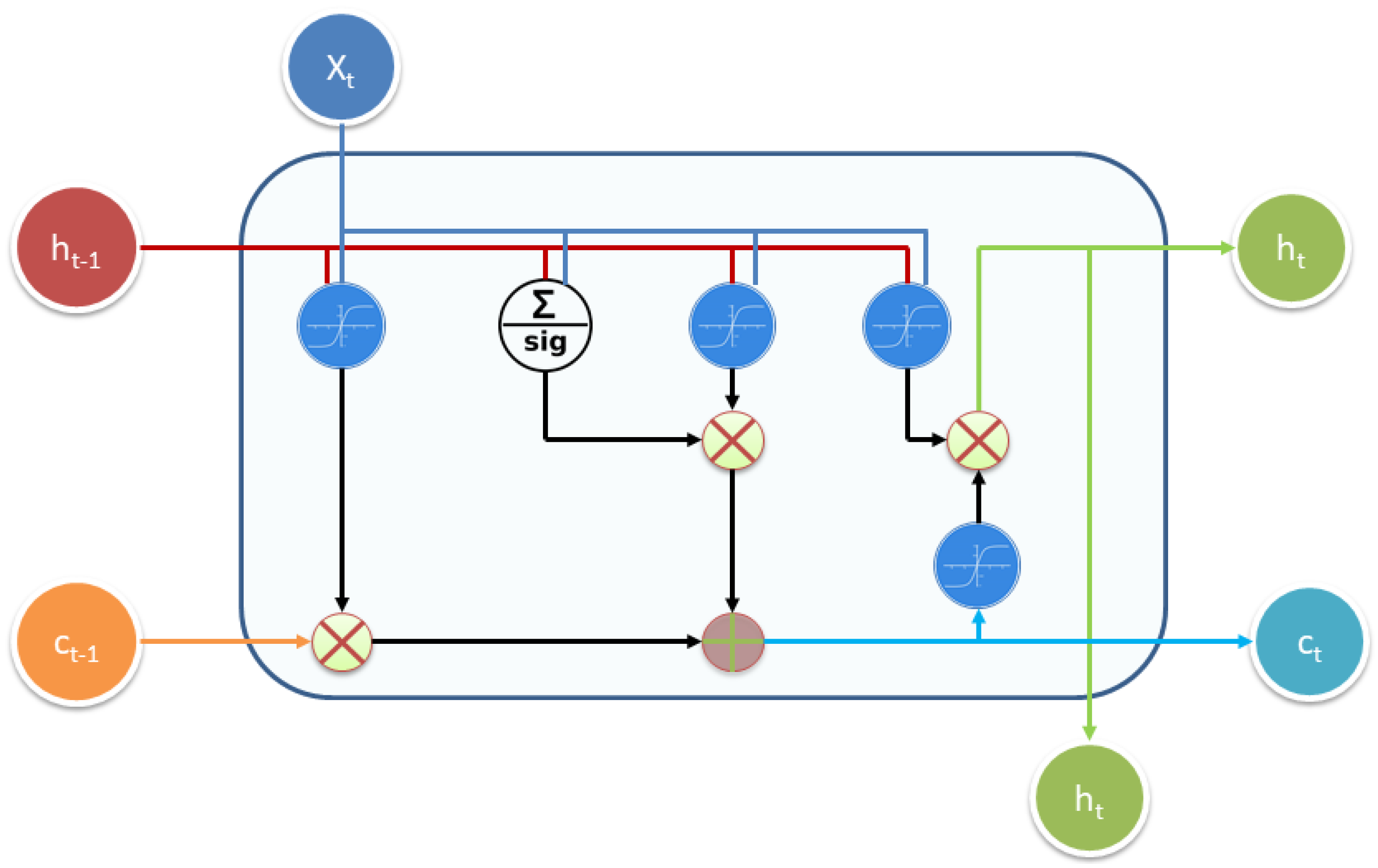
Figure 3 provides a basic diagram of the structure of a long short-term memory (LSTM) unit. At first glance, the diagram may seem complex. However, focusing on the inputs and outputs clarifies its function. The network has three primary inputs: x t , the input at the current time step; h t 1 , the output from the previous LSTM unit; and c t 1 , the “memory” from the previous unit, which is arguably the most crucial input. Regarding outputs, h t is the current unit’s output, while c t represents the current memory state. Therefore, for instance, for one single unit, the model decides by considering the current input, previous output, and previous memory. It generates a new output and alters its memory. The performed computation follows the following equations:
f t = σ c ( W f × x t + U f × h t 1 + b f ) i t = σ g ( W i × x t + U i × h t 1 + b i ) h t = σ c ( W h × x t + U h × h t 1 + b h ) c t = σ c ( W c × x t + U c × h t 1 + b c ) c t = f t c t 1 + i t c t h t = h t σ c ( c t )
where σ g and σ c are, respectively, a sigmoid and an activation function “tanh”. Let us notice that the repeated module structure can vary depending on the application as argued into [35] and the reference herein. Then, one has a model considering x t n training inputs, where n = { 1 , 2 , , n x } , with different past memories of order q = { 1 , 2 , , n q } . Furthermore, several key points should be noted from the equations:
  • These equations apply to a single time step only. They need to be recalculated for each subsequent time step.
  • The weight matrices ( W f , W i , W o , W c , U f , U i , U h , U c ) and biases ( b f , b i , b h , b c ) are fixed and do not vary with time. This implies that the same weight matrices are used across different time steps to compute the outputs.
The core concept of an LSTM network is to learn a standard representation of input data that allows for the reconstruction of the original input with minimal information loss. This is particularly useful for time series data, as LSTMs can capture temporal dependencies. Additionally, LSTM models are adept at modeling long-term dependencies and memory in time series data, making them well suited for tasks such as anomaly detection in dynamic systems like wind energy. Notably, studies such as [9,10] have highlighted the effectiveness of the LSTM model in capturing long-term dependencies by selectively updating and retrieving information, thus integrating past behavior into the diagnostic model to predict future conditions (normal or abnormal).

2.3.2. Predicting the Future Normal Expected Turbine Behavior

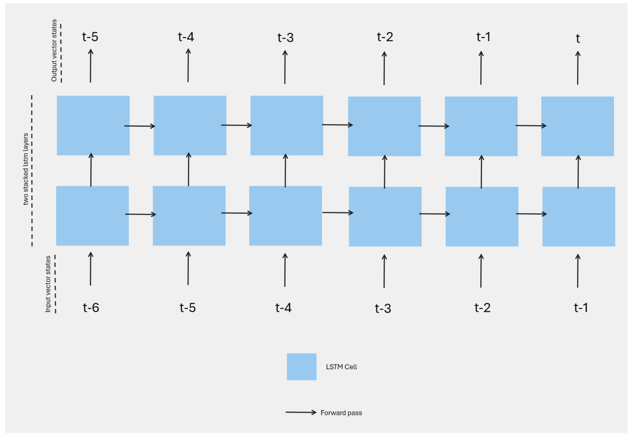
The model is trained as a sequence-to-sequence model using the available data to predict future sensor states of the system. Considering that the number of errors during the observation time is significantly narrower compared to the period when the system is functioning normally, we chose to use two stacked LSTM layers preceded by an embedding layer to encode the sensory data. The overall model architecture with the capacity to predict non-linear dynamics is presented in Figure 4 [36,37]. In its simple form and derived from relations (1), the model can be defined as follows:
h t = Γ ( x t n ) .
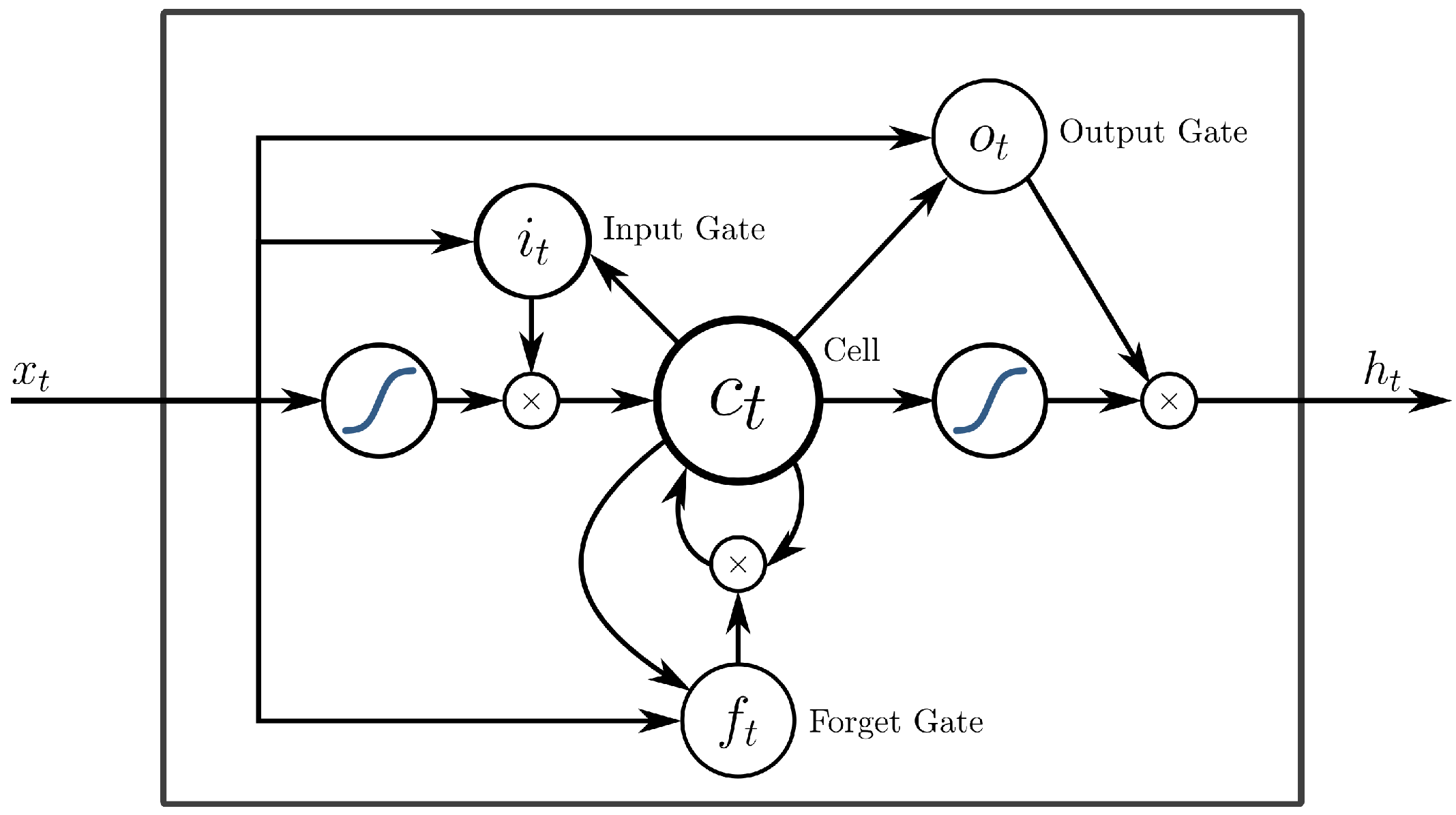
The training of the function Γ parameters is performed with a defined time window k defining the recurrent model. Then, the input sequence is defined as x t n : { S t n , S t + 1 n , , S t + k 1 n } while the output sequence is h t : { S t + 1 , S t + 2 , , S t + k } , where t is the current timestamp, and S n is the system state vector of n training inputs. As presented in Figure 5, each cell in the stacked LSTM architecture is composed by the following:
  • Input Gate i t : modulates the incorporation of input signal x t into the cell state c t [10].
  • Forget Gate f t : applies a decay factor to the cell state, allowing the model to forget irrelevant past information as depicted in [10].
  • Output Gate o t : determines the contribution of the cell state to the output signal h t [9].
  • Cell State c t : serves as the memory component of the LSTM, updated by the input and forget gates [38].
Moreover, during the training phase, we use the Huber loss function defined as:
l t = 1 2 δ ( h t h t ^ ) 2 , if | h t h t ^ | < δ | h t h t ^ | 1 2 δ , otherwise
where t is the training timestamp index, and h t and h t ^ are respectively the recorded data and the output predicted by the LSTM model. δ determines the transition point between the quadratic and linear regions of the Huber loss function. Huber loss combines the advantages from both the L1 and the mean squared error (MSE) loss functions. It prevents gradient exploding by using the L1 loss in extremities where the gradient will be independent of the error itself (constant gradient) while maintaining the smoothness of the cost function around the minimization objective.

2.3.3. Selecting Reliable Sensor Data

Let us recall that the methodology aims to assist maintenance managers and operators by simplifying and targeting their tasks to implement the appropriate maintenance strategy for specific issues. Then, to develop an effective maintenance decision support system using models like LSTM as the diagnoser, it should be transparent and comprehensible to generate explanations and provide specific inferences about the failure (including its severity and complexity) that one can validate against the domain knowledge. In this context, minimizing the input variables to be monitored is essential, as each variable can explain the event in multiple ways. Therefore, it is necessary to identify a possible subset of characteristic variables so that, for N features, the explanation of anomalies is the most plausible allowing the analysis of some statistical measurements associated with the components represented by each feature. This could simplify a targeted maintenance strategy.
The aim at this stage is to scrutinize the variables to identify those most relevant for accurately describing the behavior of a group of components. In practice, within a system with multiple components, each component typically has dedicated sensors monitoring its state. However, in wind energy systems with high levels of interconnections, a sensor designed to monitor one component may also provide valuable data for observing another component. Figure 6 illustrates an example of cross-correlation between a group of features and components. It can be observed that the behavior of each component is defined by a few key measurements, represented by different sensors M i . The objective is to select the key sensors that determine the dynamics of the global system as illustrated by the circles with red borders in the figure.
Let us note that this procedure is performed offline, so the relevant features are selected ahead of time, before real-time implementation. Furthermore, the variable selection process is carried out in two stages. First, we analyze each component separately to determine the most relevant feature using a standard Particle Swarm Optimization (PSO) algorithm. In the second stage, we apply a global optimization approach that considers the interactions among various components. The approach uses simple displacement rules to iteratively refine the number of features, progressively converging towards an optimal solution. Each iteration updates the variables based on their current velocity, the best solution found so far, and the best solutions in their neighbouring. Thus, one can ensure the identification of the most critical variables for describing the overall system behavior, while also managing time complexity and limiting the number of sensors considered.
Therefore, to effectively characterize the behavior of a group of components, we suggest iteratively identifying the optimal correlated features and influencing parameters of the entire system by examining the relationship between its component and feature. So, let us consider the subsequent clustering function g : x t 2 x t , containing measures from m sensors, defined by:
g ( x t ) = { x t m | x t m } .
Then, we can compute the component-related clustering and sensor-origin clustering η : x t C × 2 x t by the following relation:
η ( x t m ) = s Ω x t m , g x t m
with Ω ( x t m ) assigning the sub-vector state x t m to the appropriate component class such that:
arg max P ( x t m , t ) = ϕ η ( x t m ) , η ( x t n ) , with m n .
In this relation, P ( u m ( t ) , t ) represents the Pearson cross-correlation between a set of sensor m to describe the behavior of another component to which it does not directly belong. To maximize the cross-correlation, we adopt the following updating rule:
P ( x t m , t + 1 ) = λ P ( x t m , t ) + j = 1 2 c j r j ( γ t m ) .
This formulation enables a nuanced analysis of the statistical measurements concerning the components they represent that could simplify a targeted maintenance strategy. In Equation (7), r j is a random number between 0 and 1, while the constants λ and c j are specific to the PSO algorithm. The term γ m ( t ) denotes the position that has yielded the best h ( x ) value for each feature so far. These positions are updated with each iteration to reflect the optimal feature settings ( h * ( x ) = d ) discovered up to that point.
Lastly, since multiple features are evaluated to identify the optimal solution, each feature can be updated concurrently. It is sufficient to collect the updated values for each iteration. To ensure the convergence of the optimal cross-correlation, one verifies whether the global cross-correlation between each attribute and feature meets the required criteria.
Then,
P q ( x t m , t ) Λ Break , Otherwise Continue
where Λ represents the performance desired and defined for the experiment and q = 1 , , n q is the iteration number allowing us to verify condition (8).
Once persistent sensors are determined, one can follow the dynamic behavior of the system by the following metric. Let us define Δ S t m , for a given sensor indexed with m at timestamp t, the deviation estimating how unusual or unexpected the observed data are for the learned ordinary turbine functioning manifold:
Δ S t m = i = 0 p ( d i , t m d ^ i , t m ) 2 .
Then, anomalies are defined using the following rule:
ϵ t m = 1 , if Δ S t m τ m : abnormal situation 0 , otherwise
In these equations, p is the number of features in the sub-vector state, i defines the i t h element of the sub-vector. τ m is a threshold determined empirically and depends on the model prediction accuracy. In other terms, if the diagnoser model accurately represents the system’s behavior and the most relevant features well describe the abnormal situation, the threshold can be adjusted empirically to reduce false alarms.

2.3.4. Failure Analysis and Processing

As the previous system helps us understand and identify the primary influential factors contributing to the root cause of a failure, it becomes feasible to enhance both the diagnosis and precluding future incidents by leveraging the dynamics inherent in each variable. Consequently, one can analyze the divergence, d r , to transition the input variable d r from a faulty operating state to normal operating one d r ˜ by considering the following expressions:
d r = ( d ˜ r d r )
where d ˜ and d represent the relearned and faulted input vectors, respectively, and r denotes the number of remaining features that most significantly contribute to the anomaly.
By examining these divergences, the contribution of each feature to the occurrence of faults can be explained. The proportion of the contribution of the ith input variable to all deviations is given by [18]:
C t i = d i t j = 1 r d t j 100
Finally, all these outputs of the diagnoser model are now coupled with a VR application that simulates in real time the wind farm behavior and displays automatically identified faults (detected and localized). When the diagnoser model identifies an anomaly (according to relation (10)), the diagnoser server sends it to the Unity server, which checks if this anomaly has already occurred on the associated turbine or not. If this is the case, we assess whether the time frame between the most recent occurrence of the anomaly and its current manifestation is within a certain threshold (limit of the occurrence number during the observation). The persistence indicator over time is calculated by counting the number of times s τ the jth relevant feature crosses the limited threshold within a sliding window of length k as follows:
p j , t = 1 k × τ = t ( k 1 ) t s j , τ
Depending on the result of this calculation, the irregularity increases and may become significant, thus becoming critical above a certain threshold. Depending on the presence and risk level of an anomaly, the parameter concerned is displayed in a specific color. In this paper, “WHITE” defines normal behavior, “ORANGE” a warning, and “RED” a critical anomaly. The maintenance manager can use this information to identify and prevent future critical faults.

3. Results and Discussion

In this paper, we apply the methodology for wind farm monitoring by designing a customized head-mounted fault display system that integrates predictive capabilities (through deep learning models) with anomaly explanations (focusing on model transparency and comprehensibility) for effective predictive maintenance tasks.
Wind farms are essentially composed of a set of wind turbines which convert kinetic wind energy into mechanical energy, which is then transformed into electrical energy for various uses (Figure 7). These turbines are crucial for the renewable energy infrastructure, providing a sustainable and environmentally friendly alternative to fossil fuels. They play a major role in the transition to renewable energy by harnessing wind power to generate clean electricity, contributing to a sustainable and resilient energy future. Despite facing challenges, advancements in technology and increasing efficiency continue to make wind energy an integral part of the global energy landscape. However, wind turbines are complex systems susceptible to faults that can impact performance and increase maintenance costs. For example, issues in the hydraulic system, such as pressure drops or air content in the oil, and sensor failures that measure various parameters can stem from electrical or mechanical problems, each affecting turbine operation differently. In this context, it is essential to assist maintenance managers and operators by simplifying and targeting their tasks to implement the appropriate maintenance strategy for specific issues. That involves first determining the persistent features that allow the observation of each component’s behavior, which is necessary for generating explanations and drawing specific inferences about the failure.
The dataset provided by Energias De Portugal (https://www.edp.com/en/innovation/open-data (accessed on 25 March 2024)) is utilized for the computation test of the methodology. It includes measurements from multiple wind turbines, recorded every ten minutes over a two-year period, from 1 January 2016 to 1 September 2017, totaling 87,208 samples per turbine. The dataset features 81 sensors distributed across 12 turbine components (such as the gearbox, generator, and transformer) as well as environmental factors (including wind speed, wind direction, and ambient temperature). Statistical metrics like standard deviation, minimum and maximum values, average sensor observations, and signal descriptors provide comprehensive insights.

3.1. Diagnoser Model Validation

The effectiveness of the methodology is primarily ensured by the performance of the diagnoser. The accuracy of the forecasting model is critical, with the error needing to be as low as possible for effective anomaly detection.
The diagnoser model is developed using the following process: 80% of the available data, comprising 350,764 training examples, are used. The model is trained with a batch size of 256 over 300 epochs, utilizing stochastic gradient descent as the optimizer. The δ parameter in the Huber loss function is tuned in a cross-validation manner. We keep δ = 1 to limit the influence of some part of our data points which poorly fit the model. As shown in Table 1, the model’s performance exceeds the requirements for the anomaly detection task, achieving a mean squared error (MSE) of 0.18. The table also presents the model’s mean absolute error (MAE) and mean relative error (MRE) metrics for selected features.
Using these statistical metrics, thresholds can be proposed for each variable. If these thresholds are exceeded, according to Equation (10), the behavior of the variable is deemed abnormal, indicating potential failures in the related functionalities. The lower the MRE for each variable, the better the system can distinguish between normal and abnormal behaviors.

3.2. Fault Diagnosis

The service record document failures highlight five critical electrical and mechanical components—namely, the gearbox, generator, generator bearing, transformer, and hydraulic unit. These failures occurred on various dates across multiple wind turbines. Additionally, the study incorporates reports detailing 22 errors in various turbine parts, including transformers, generators, and hydraulic groups. The failure observed for the turbine number 7 is detailed in Table 2.
In what follows, we propose to discuss the relationships between the identified anomalies and reported faults to identify and locate faults. In Figure 8, the first reported error is marked with a vertical dashed line, and anomalies detected in each principal component are represented by dots using our approach. Before the error on 30 April 2016, multiple anomalies in the nacelle direction were detected, indicating a failure in regulating the turbine direction according to the wind. This could be due to natural wind direction irregularities in an offshore context or a mismatch in the regulation latency with wind direction variations, leading to asymmetrical stress on the blades and increased generator bearing temperature.
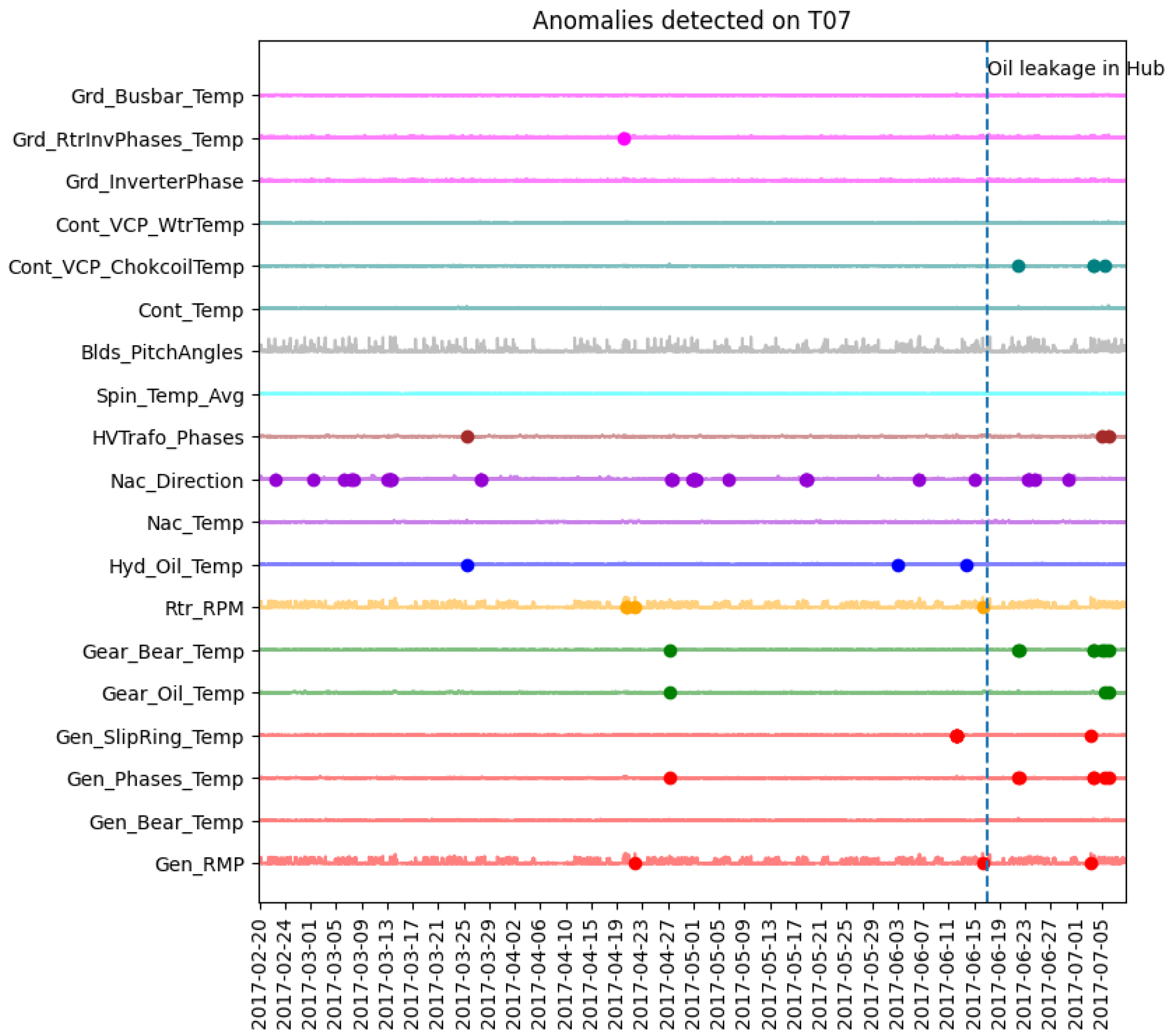
Figure 9 shows the system issuing alerts for wind turbine components before detecting an oil leakage in the hub on 12 March 2019 (marked by a vertical dashed line). The hub, central to the rotor with attached blades, experienced oil leakage, suggesting a potential issue with the hydraulic system that uses oil to transmit power and pressure to actuators. An oil leakage can impair the hydraulic system’s functionality and efficiency, causing damage to the components. Before the leakage, the system detected an anomaly in the hydraulic oil temperature, represented by blue dots on the graph. Maintaining optimal oil temperature is crucial for performance and viscosity. Deviations can affect fluid flow and pressure, leading to issues like cavitation, corrosion, and wear, potentially contributing to oil leakage.
Additionally, alerts were issued for the generator SlipRing temperature, shown in red on the graph. The SlipRing enables electrical power and signal transmission between the rotating and stationary parts of the generator. Elevated SlipRing temperatures may indicate malfunctions or poor contact, leading to sparks, arcs, electrical noise, and generator damage. Such damage can affect oil quality and viscosity, potentially contributing to oil leakage from the generator [39].
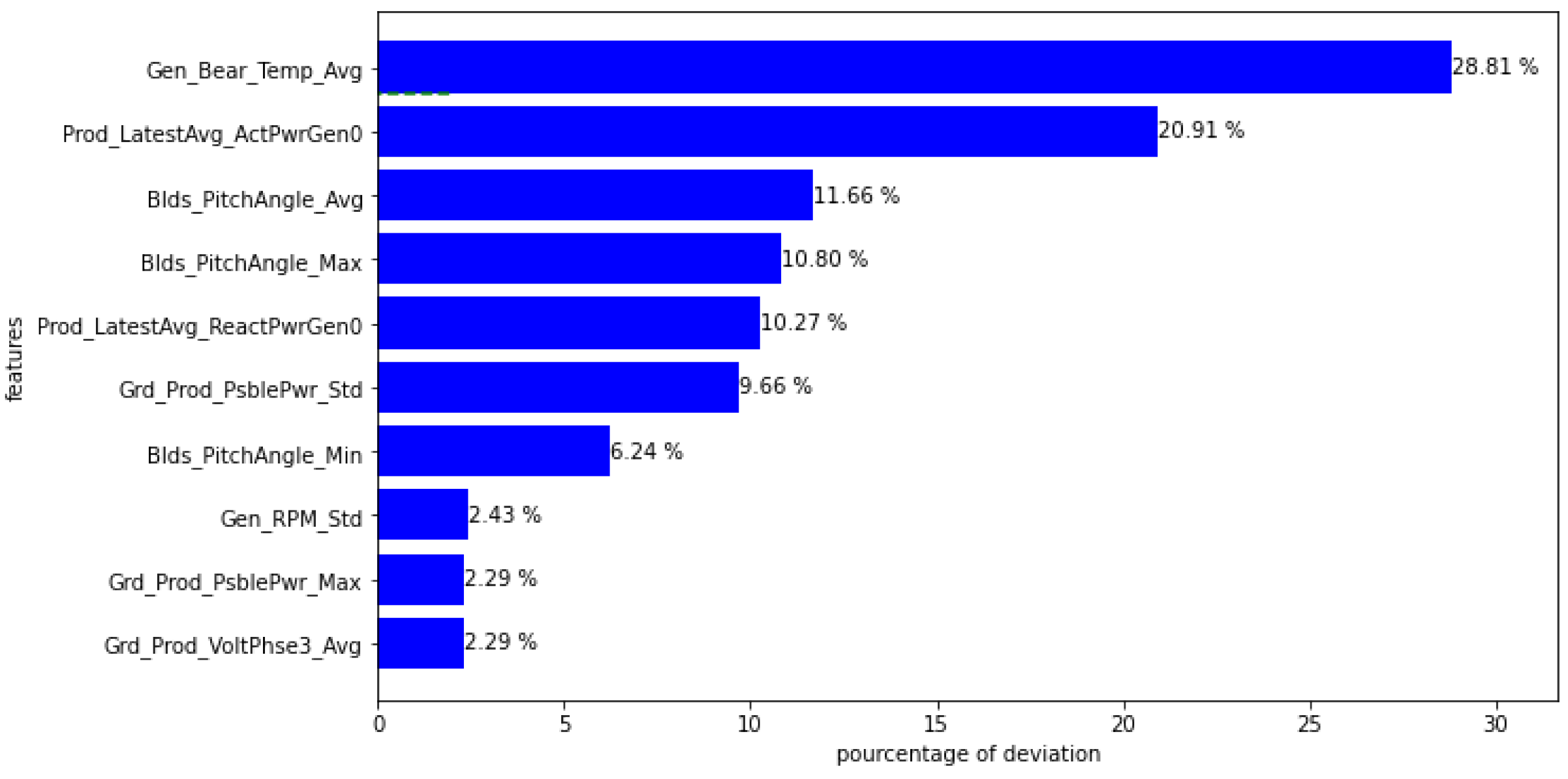
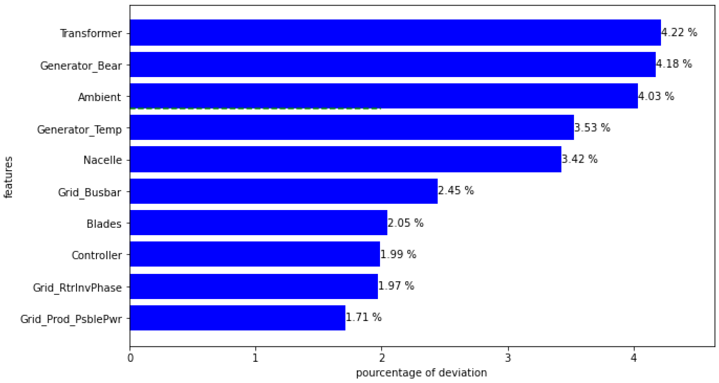
Each parameter can be analyzed and compared to see which deviates the most according to the investigated anomaly (cf. Section 2.3.4). Two scenarios are considered in Figure 10 and Figure 11. In Figure 10, the system alerted operators to a significant rise in the generator bearings’ temperature. Conversely, Figure 11 shows a significant deviation in three wind turbine components: the transformer, generator bearings, and ambient temperature. Initially considered a warning anomaly, this could escalate to a critical anomaly if the deviations persist, according to Equation (13).
Histograms inform maintenance operators about any deviations of each feature from its normal value. Figure 10 illustrates the detection of an anomaly and a significant temperature increase in the generator bearings. Figure 11 provides an example, where significant deviations in the transformer, generator bearings, and ambient temperature are observed.
The results are clear: not all variables are affected by a given problem, regardless of the failed component. This underscores the rationale for minimizing the number of characteristics to be observed while maximizing the relationships each variable may have with a specific issue.

3.3. Persistent Feature Selection

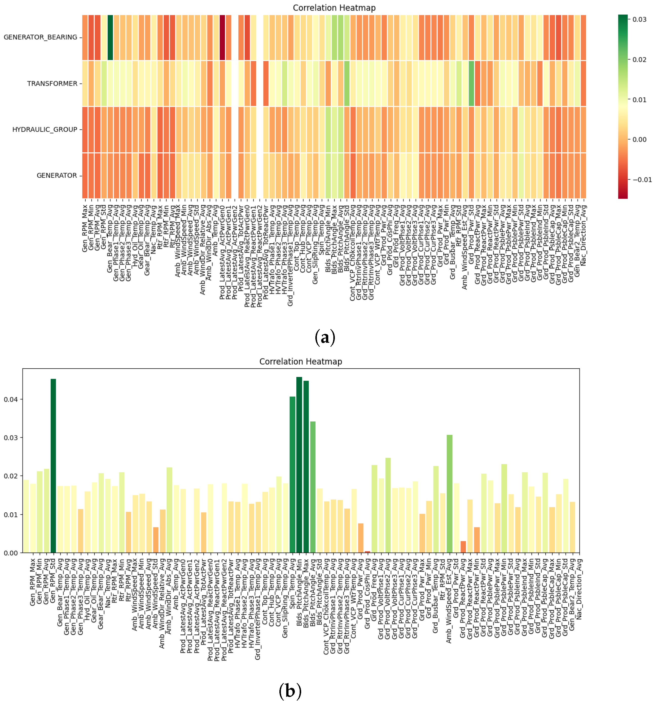
To identify the impact of individual features, we conduct a correlation study between the 81 available features and the recorded problems as detailed in Section 2.3.3. Figure 12 presents a heat map illustrating the correlation between each feature (x-axis) and problems related to specific components (y-axis).
The heat map reveals a high correlation between problems related to the generator bearing and the recorded temperature of the generator bearing. Consequently, for this example, all features that do not meet a minimum correlation threshold with our targets are omitted from the rest of the study to refine the findings.
These initial insights indicate that certain variables are more influential than others. Highly correlated variables are directly related to the occurrence of errors, making the results intuitive and explainable. By applying an arbitrary threshold, we streamline the detection model, reducing the number of variables from 81 to 21 (Table 3).

3.4. Customized HMFD Application

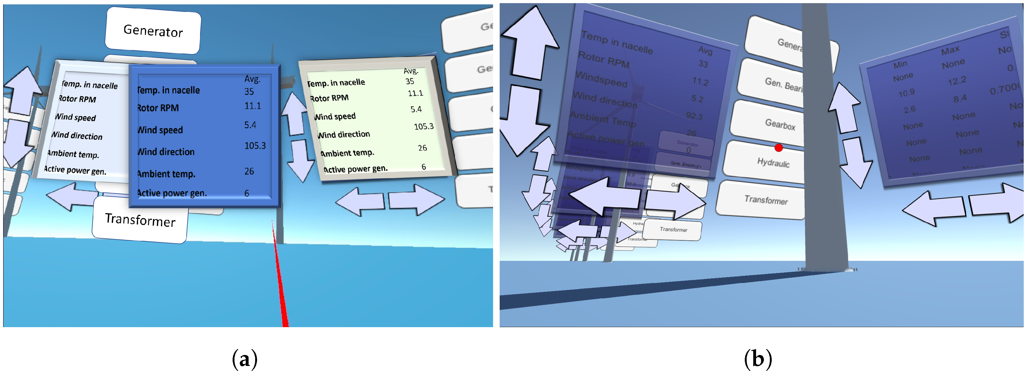
The final stage in our methodology is the integration of the insights presented above into the VR application. The application functions similarly on both the computer and the headset versions, ensuring accessibility even if no functional headset is available. The primary difference between the two versions lies in the movement and interaction controls. Figure 13 illustrates this interaction and the user’s placement within a 3D model representation of a wind turbine field. Each turbine is accompanied by a panel displaying readings from various common turbine sensors and a set of buttons allowing the user to navigate different locations within the wind turbine. Interaction relies on controllers emitting rays, like the red one shown in Figure 13, with the weather data display following the position of the left controller.
The HMFD interaction method, demonstrated in Figure 13a, uses controllers emitting rays, while the computer version uses a simple cursor, represented by the red circle in Figure 13b. Inside a wind turbine, users can view models of central units, including generators and transformers, providing access to data linked to specific components.
Figure 14a illustrates the detection of anomalies on a wind turbine component. The potentially faulty component is highlighted with a particle effect. When one wants to display the data associated with sensors whose behavior is abnormal, one highlights them by changing the writing color. If the user is outside a wind turbine, detected anomalies are displayed as shown in Figure 14b,c. In this scenario, a generator anomaly is indicated by the red highlighting of the button granting access to it. While comparing Figure 14b,c, two levels of anomaly detection become apparent. Figure 14b represents a typical warning, while Figure 14c indicates a critical anomaly, escalating from a warning due to frequent occurrences. In this example, critical errors are defined as anomalies that occur 7 times in the last 30 days.
Using this information, maintenance operators can promptly decide whether to investigate further on site or replace a part, thus saving time.

4. Conclusions

This paper presented a proof of concept for using explainable artificial intelligence to enhance head-mounted fault display systems. To help operators understand the importance of their tasks, we provide information on the parameters causing problems and their criticality. We introduce a novel approach to evaluate the contribution of each feature to all possible subsets of other features. Additionally, the integrated diagnoser model enables early identification and localization of anomalies. By linking identified anomalies with manually recorded problems, we provide valuable insights to the maintenance manager.
The prediction model shows satisfactory forecasting accuracy (around 7%) across various components but can be further improved by leveraging meteorological data and refining the model architecture and hyperparameters. The system effectively detects issues before they occur and operates efficiently without GPU support. It has also proven capable of detecting most reported issues well in advance, alerting relevant components, and running efficiently on lightweight models without needing GPU support.
Future work could explore other sequence-to-sequence architectures, such as transformers, which could enhance prediction accuracy and reduce false alarms due to their effectiveness in current state-of-the-art tasks like speech recognition and language models. Additionally, the system could evolve from a decision-aid tool to a complete decision-maker. By conducting a more in-depth analysis of the relationship between anomalies and critical faults, the model could provide prescriptions and the actions required to maintain wind farm operations rather than merely serving as an alert system.

Author Contributions

Conceptualization: A.B. and L.R. Methodology: L.R. Software: A.B. and L.C. Validation: L.R. Formal analysis: A.B., L.C. and L.R. Investigation: A.B. and L.C. Data curation: A.B. and L.R. Writing—original draft preparation: A.B., L.C. and L.R. Writing—review and editing: A.B. and L.R. Project administration: L.R. All authors have read and agreed to the published version of the manuscript.

Funding

This document is the result of the research in the framework of the XPM (eXplainable Predictive Maintenance) project funded by the French National Research Agency (ANR-21-CHR4-0003) under the CHIST-ERA program (CHIST-ERA-19-XAI-012).

Data Availability Statement

In this paper we use open data available on: https://www.edp.com/en/innovation/open-data (accessed on 25 March 2024).

Conflicts of Interest

The authors declare no conflicts of interest. The funders had no role in the design of the study; in the collection, analyses, or interpretation of data; in the writing of the manuscript; or in the decision to publish the results.

Abbreviations

The following abbreviations are used in this manuscript:
VRVirtual reality
ARAugmented reality
MSEMean squared error
MAEMean absolute error
MREMean relative error
HMFDHead mounted fault display
AIArtificial Intelligence
XPMeXplainable Predictive Maintenance
XAIeXplainable Artificial Intelligence
SHAPSHapley Additive exPlanation
LIMELocal Interpretable Model-Agnostic Explanations
DBSCANDensity-Based Spatial Clustering of Applications with Noise
LUXLocal Uncertain Explanation
LORELOcal Rule-based Explanation
PdMPredictive Maintenance
LSTMLong short-term memory
PSOParticle Swarm Optimization
PoCProof of concept
RNNRecursive neural network
HMIHuman–machine interface

References

  1. Udo, W.; Muhammad, Y. Data-Driven Predictive Maintenance of Wind Turbine Based on SCADA Data. IEEE Access 2021, 9, 162370–162388. [Google Scholar] [CrossRef]
  2. Sayed-Mouchaweh, M.; Rajaoarisoa, L. Explainable Decision Support Tool for IoT Predictive Maintenance within the context of Industry 4.0. In Proceedings of the 21st IEEE ICMLA, Nassau, Bahamas, 12–14 December 2022; pp. 1492–1497. [Google Scholar] [CrossRef]
  3. Fitouri, C.; Fnaiech, N.; Varnier, C.; Fnaiech, F.; Zerhouni, N. A Decison-Making Approach for Job Shop Scheduling with Job Depending Degradation and Predictive Maintenance. IFAC-PapersOnLine 2016, 49, 1490–1495. [Google Scholar] [CrossRef]
  4. Gow, R.; Rabhi, F.A.; Venugopal, S. Anomaly detection in complex real-world application systems. IEEE TNSM 2017, 15, 83–96. [Google Scholar] [CrossRef]
  5. Zhang, J.; Wang, P.; Yan, R.; Gao, R.X. Deep Learning for Improved System Remaining Life Prediction. Procedia CIRP 2018, 72, 1033–1038. [Google Scholar] [CrossRef]
  6. Rhodes, J.S. Supervised Manifold Learning via Random Forest Geometry-Preserving Proximities. arXiv 2023, arXiv:2307.01077. [Google Scholar]
  7. Wang, H.; Yao, L.; Wang, H.; Liu, Y.; Li, Z.; Wang, D.; Hu, R.; Tao, L. Supervised Manifold Learning Based on Multi-Feature Information Discriminative Fusion within an Adaptive Nearest Neighbor Strategy Applied to Rolling Bearing Fault Diagnosis. Sensors 2023, 23, 9820. [Google Scholar] [CrossRef] [PubMed]
  8. Jain, P.; Bajpai, M.; Pamula, R. A Modified DBSCAN Algorithm for Anomaly Detection in Time-Series Data with Seasonality. Int. Arab JIT 2022, 19, 23–28. [Google Scholar] [CrossRef] [PubMed]
  9. Van Houdt, G.; Mosquera, C.; Nápoles, G. A review on the long short-term memory model. Artif. Intell. Rev. 2020, 53, 5929–5955. [Google Scholar] [CrossRef]
  10. Yu, Y.; Si, X.; Hu, C.; Zhang, J. A Review of Recurrent Neural Networks: LSTM Cells and Network Architectures. Neural Comput. 2019, 31, 1235–1270. [Google Scholar] [CrossRef]
  11. Rajaoarisoa, L.; Kuk, M.; Bobek, S.; Sayed-Mouchaweh, M. Hybrid and co-learning approach for anomalies prediction and explanation of wind turbine systems. Eng. Appl. Artif. Intell. 2024, 133, 108046. [Google Scholar] [CrossRef]
  12. Bobek, S.; Nowaczyk, S.; Gama, J.; Pashami, S.; Ribeiro, R.P.; Taghiyarrenani, Z.; Veloso, B.; Rajaoarisoa, L.; Szelazėk, M.; Nalepa, G.J. Why Industry 5.0 Needs XAI 2.0? In Proceedings of the Conference on eXplainable Artificial Intelligence (xAI-2023), Lisbon, Portugal, 26–28 July 2023. [Google Scholar]
  13. Ribeiro, M.T.; Singh, S.; Guestrin, C. Anchors: High-precision model-agnostic explanations. In Proceedings of the Thirty-Second AAAI Conference on Artificial Intelligence and Thirtieth Innovative Applications of Artificial Intelligence Conference and Eighth AAAI Symposium on Educational Advances in Artificial Intelligence (AAAI’18/IAAI’18/EAAI’18), New Orleans, LA, USA, 2–7 February 2018; pp. 1527–1535. [Google Scholar]
  14. Ribeiro, M.T.; Singh, S.; Guestrin, C. “Why Should I Trust You?”: Explaining the Predictions of Any Classifier. In Proceedings of the 22nd ACM SIGKDD International Conference on Knowledge Discovery and Data Mining (KDD ’16), New York, NY, USA, 13–17 August 2016; pp. 1135–1144. [Google Scholar] [CrossRef]
  15. Guidotti, R.; Monreale, A.; Ruggieri, S.; Pedreschi, D.; Turini, F.; Giannotti, F. Local Rule-Based Explanations of Black Box Decision Systems. arXiv 2018, arXiv:1805.10820[cs]. [Google Scholar] [CrossRef]
  16. Bobek, S.; Nalepa, G.J. Introducing Uncertainty into Explainable AI Methods. In Proceedings of the Computational Science—ICCS 2021, Krakow, Poland, 16–18 June 2021; Paszynski, M., Kranzlmüller, D., Krzhizhanovskaya, V.V., Dongarra, J.J., Sloot, P.M.A., Eds.; Springer International Publishing: Cham, Switzerland, 2021; pp. 444–457. [Google Scholar]
  17. Lundberg, S.M.; Erion, G.; Chen, H.; DeGrave, A.; Prutkin, J.M.; Nair, B.; Katz, R.; Himmelfarb, J.; Bansal, N.; Lee, S.I. From local explanations to global understanding with explainable AI for trees. Nat. Mach. Intell. 2020, 2, 56–67. [Google Scholar] [CrossRef]
  18. Randriarison, J.; Rajaoarisoa, L.; Sayed-Mouchaweh, M. Faults explanation based on a machine learning model for predictive maintenance purposes. In Proceedings of the 7th Edition in the Series of the International Conference on Control, Automation and Diagnosis, Rome, Italy, 10–12 May 2023; pp. 01–06. [Google Scholar] [CrossRef]
  19. Selvaraju, R.R.; Das, A.; Vedantam, R.; Cogswell, M.; Parikh, D.; Batra, D. Grad-CAM: Why did you say that? Visual Explanations from Deep Networks via Gradient-based Localization. arXiv 2016, arXiv:1610.02391. [Google Scholar]
  20. Rudin, C. Stop explaining black box machine learning models for high stakes decisions and use interpretable models instead. Nat. Mach. Intell. 2019, 1, 206–215. [Google Scholar] [CrossRef] [PubMed]
  21. Lou, Y.; Caruana, R.; Gehrke, J.; Hooker, G. Accurate Intelligible Models with Pairwise Interactions. In Proceedings of the 19th ACM SIGKDD International Conference on Knowledge Discovery and Data Mining (KDD ’13), New York, NY, USA, 11–14 August 2013; pp. 623–631. [Google Scholar] [CrossRef]
  22. Kuk, M.; Bobek, S.; Veloso, B.; Rajaoarisoa, L.; Nalepa, G.J. Feature Importances as a Tool for Root Cause Analysis in Time-Series Events. In Proceedings of the Computational Science—ICCS 2023, Prague, Czech Republic, 3–5 July 2023; Mikyška, J., de Mulatier, C., Paszynski, M., Krzhizhanovskaya, V.V., Dongarra, J.J., Sloot, P.M., Eds.; Springer Nature: Cham, Switzerland, 2023; pp. 408–416. [Google Scholar] [CrossRef]
  23. Kostoláni, M.; Murín, J.; Kozák, Š. Intelligent predictive maintenance control using augmented reality. In Proceedings of the 22nd ICPC19, Strbske Pleso, Slovakia, 11–14 June 2019; pp. 131–135. [Google Scholar] [CrossRef]
  24. Cachada, A.; Barbosa, J.; Leitño, P.; Gcraldcs, C.A.; Deusdado, L.; Costa, J.; Teixeira, C.; Teixeira, J.; Moreira, A.H.; Moreira, P.M.; et al. Maintenance 4.0: Intelligent and Predictive Maintenance System Architecture. In Proceedings of the 2018 IEEE 23rd International Conference on Emerging Technologies and Factory Automation (ETFA), Torino, Italy, 4–7 September 2018; Volume 1, pp. 139–146. [Google Scholar] [CrossRef]
  25. Alves, F.; Badikyan, H.; Antonio Moreira, H.J.; Azevedo, J.; Moreira, P.M.; Romero, L.; Leitao, P. Deployment of a Smart and Predictive Maintenance System in an Industrial Case Study. In Proceedings of the 2020 IEEE 29th International Symposium on Industrial Electronics (ISIE), Delft, The Netherlands, 17–19 June 2020; pp. 493–498. [Google Scholar] [CrossRef]
  26. Wolfartsberger, J.; Zenisek, J.; Wild, N. Data-Driven Maintenance: Combining PdM and Mixed Reality-Supported Remote Assistance. Procedia Manuf. 2020, 45, 307–312. [Google Scholar] [CrossRef]
  27. Bouzidi, A.; Claeys, L.; Randrianandraina, R.; Rajaoarisoa, L.; Wannous, H.; Sayed-Mouchaweh, M. Deep learning for a customised head-mounted fault display system for the maintenance of wind turbines. In Proceedings of the 2024 International Conference on Control, Automation and Diagnosis (ICCAD), Paris, France, 15–17 May 2024; pp. 1–6. [Google Scholar] [CrossRef]
  28. Alm, C. Language as Sensor in Human-Centered Computing: Clinical Contexts as Use Cases. Lang. Linguist. Compass 2016, 10, 105–119. [Google Scholar] [CrossRef]
  29. Hanheide, M.; Bauckhage, C.; Sagerer, G. Combining environmental cues & head gestures to interact with wearable devices. In Proceedings of the 7th International Conference on Multimodal Interfaces, ICMI ’05, New York, NY, USA, 4–6 October 2005; pp. 25–31. [Google Scholar] [CrossRef]
  30. Luo, H.; Du, J.; Yang, P.; Shi, Y.; Liu, Z.; Yang, D.; Zheng, L.; Chen, X.; Wang, Z.L. Human–Machine Interaction via Dual Modes of Voice and Gesture Enabled by Triboelectric Nanogenerator and Machine Learning. ACS Appl. Mater. Interfaces 2023, 15, 17009–17018. [Google Scholar] [CrossRef] [PubMed]
  31. Wambsganss, T. Designing Adaptive Argumentation Learning Systems Based on Artificial Intelligence. In Proceedings of the Extended Abstracts of the 2021 CHI Conference on Human Factors in Computing Systems (CHI EA ’21), New York, NY, USA, 8–13 May 2021. [Google Scholar] [CrossRef]
  32. Kyösti, P.; Reed, S.; Sjödin, S. A Decision Support Tool for Optimising Support Site Configuration of Functional Products. Procedia CIRP 2014, 22, 175–180. [Google Scholar] [CrossRef]
  33. Galanti, R.; de Leoni, M.; Monaro, M.; Navarin, N.; Marazzi, A.; Di Stasi, B.; Maldera, S. An explainable decision support system for predictive process analytics. Eng. Appl. Artif. Intell. 2023, 120, 105904. [Google Scholar] [CrossRef]
  34. Lachekhab, F.; Benzaoui, M.; Tadjer, S.A.; Bensmaine, A.; Hamma, H. LSTM-Autoencoder Deep Learning Model for Anomaly Detection in Electric Motor. Energies 2024, 17, 2340. [Google Scholar] [CrossRef]
  35. Kothadiya, D.; Bhatt, C.; Sapariya, K.; Patel, K.; Gil-González, A.B.; Corchado, J.M. Deepsign: Sign Language Detection and Recognition Using Deep Learning. Electronics 2022, 11, 1780. [Google Scholar] [CrossRef]
  36. Lindemann, B.; Müller, T.; Vietz, H.; Jazdi, N.; Weyrich, M. A survey on long short-term memory networks for time series prediction. Procedia CIRP 2021, 99, 650–655. [Google Scholar] [CrossRef]
  37. Siami-Namini, S.; Tavakoli, N.; Namin, A.S. The performance of LSTM and BiLSTM in forecasting time series. In Proceedings of the 2019 IEEE International Conference on Big Data (Big Data), Los Angeles, CA, USA, 24 February 2020; IEEE: Piscataway, NJ, USA, 2019; pp. 3285–3292. [Google Scholar]
  38. Staudemeyer, R.C.; Morris, E.R. Understanding LSTM—A tutorial into long short-term memory recurrent neural networks. arXiv 2019, arXiv:1909.09586. [Google Scholar]
  39. Teimourzadeh Baboli, P.; Babazadeh, D.; Raeiszadeh, A.; Horodyvskyy, S.; Koprek, I. Optimal temperature-based condition monitoring system for wind turbines. Infrastructures 2021, 6, 50. [Google Scholar] [CrossRef]
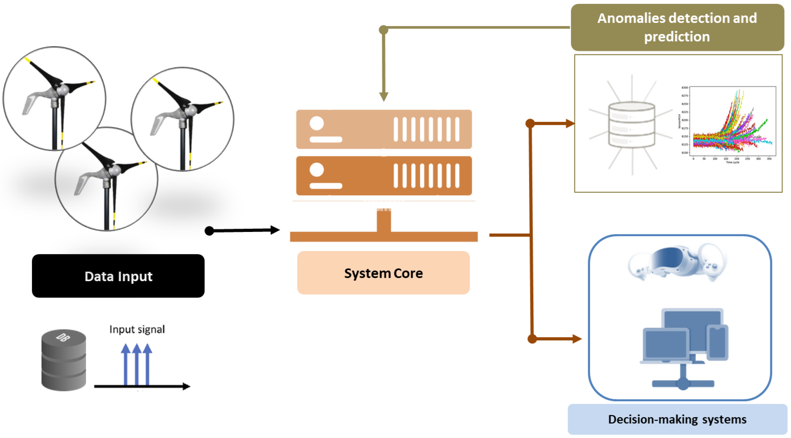
Figure 1. Real-time head-mounted fault system architecture [27].
Futureinternet 16 00282 g001
Figure 2. Example of the human–machine interface view both on the computer and the headset systems.
Futureinternet 16 00282 g002
Figure 3. The basic diagram of the long short-term memory (LSTM) neural network [35].
Futureinternet 16 00282 g003
Figure 4. Diagnoser model architecture.
Futureinternet 16 00282 g004
Figure 5. Standard simplified diagram of an LSTM cell.
Futureinternet 16 00282 g005
Figure 6. Relationship example between a group of features vs. a group of components.
Futureinternet 16 00282 g006
Figure 7. Wind turbine systems with their different components.
Futureinternet 16 00282 g007
Figure 8. Detected anomalies before the first reported malfunction of the turbine T07 (generator bearing).
Futureinternet 16 00282 g008
Figure 9. Detected anomalies before the third reported malfunction of the turbine T07 (hydraulic group).
Futureinternet 16 00282 g009
Figure 10. Detection and explanation of a significant rise in the generator bearings’ temperature.
Futureinternet 16 00282 g010
Figure 11. Detection and explanation of a rise in the transformer’s temperature.
Futureinternet 16 00282 g011
Figure 12. Correlations between each feature and instances of system malfunction. (a) For each component. (b) Zoom display with the generator bearing component.
Futureinternet 16 00282 g012
Figure 13. Windfarm monitoring clients’ views: (a) HMFD interface, (b) PC interface.
Futureinternet 16 00282 g013
Figure 14. (a) Detected warning view in generator component. (b) Warning anomaly view in the windfarm. (c) Critical anomaly view in the windfarm.
Futureinternet 16 00282 g014
Table 1. Prediction accuracy of some of the variables [27].
ComponentVariableAverage ValueMAEMRE
GeneratorRotation per Minute1121.7495.188.48%
GeneratorBearing Temperature48.463.637.5%
GeneratorPhase 1 Temperature63.103.415.4%
GeneratorPhase 2 Temperature63.592.964.66%
GeneratorPhase 3 Temperature63.312.894.57%
Hydraulic groupOil Temperature34.461.163.38%
Gear boxOil Temperature49.201.653.36%
Gear boxBearing Temperature54.762.234.07%
Table 2. Example maintenance records for turbine number 07.
Turbine IDComponentTimestampRemarks
T07GENERATOR_BEARING30 April 2016 T12:40:00High temperature in generator bearing (replaced sensor)
TRANSFORMER10 July 2016 T03:46:00High-temperature transformer
TRANSFORMER23 August 2016 T02:21:00High-temperature transformer. Transformer refrigeration repaired
HYDRAULIC_GROUP17 June 2017 T11:35:00Oil leakage in hub
GENERATOR_BEARING20 August 2017 T06:08:00Generator bearings damaged
GENERATOR21 August 2017 T14:47:00Generator damaged
Table 3. The 21st top variables required for the test [11].
Feature IDComponentFeature DescriptorUnitFeature Description
01GeneratorGen_RPM_Max[rpm]Maximum generator rpm in latest average period
02GeneratorGen_RPM_Std[rpm]Std. generator rpm in latest average
03GeneratorGen_Phase1_Temp_Avg[°C]Average temperature inside generator in stator windings phase 1
04GeneratorGen_Phase3_Temp_Avg[°C]Average temperature inside generator in stator windings phase 3
05GeneratorHyd_Oil_Temp_Avg[°C]Oil Average temperature in Humidification system
06RotorRtr_RPM_Avg[rpm]Average speed of the Rotor
07ProductionProd_LatestAvg_ActPwrGen0[Wh]Active power - generator disconnected (yaw motor hydraulic motor etc.)
08ProductionProd_LatestAvg_ActPwrGen1[Wh]Active power—generator connected in delta
09ProductionProd_LatestAvg_ActPwrGen2[Wh]Active power—generator connected in star
10TransformerHVTrafo_Phase1_Temp_Avg[°C]Average temperature in HV transformer phase L1
11TransformerHVTrafo_Phase2_Temp_Avg[°C]Average temperature in HV transformer phase L2
12GridGrd_InverterPhase1_Temp_Avg[°C]Average temperature measured by the IGBT-driver on the grid side inverter
13SpinnerSpin_Temp_Avg[°C]Average temperature in the nose cone
14BladesBlds_PitchAngle_Min[°]Average angle
15ControllerCont_VCP_WtrTemp_Avg[°C]Average temperature on the VCP-board
16GridGrd_Prod_ReactPwr_Max[kVAr]Maximum grid reactive power
17GridGrd_Prod_PsblePwr_Max[kW]Maximum possible grid active power
18GridGrd_Prod_PsbleInd_Max[kVar]Maximum possible inductive reactive power
19GridGrd_Prod_PsbleCap_Max[kVar]Maximum possible capacitive reactive power
20GridGrd_Prod_CurPhse2_Avg[A]Averaged current in phase 2
21GridGrd_Prod_CurPhse3_Avg[A]Averaged current in phase 3
Disclaimer/Publisher’s Note: The statements, opinions and data contained in all publications are solely those of the individual author(s) and contributor(s) and not of MDPI and/or the editor(s). MDPI and/or the editor(s) disclaim responsibility for any injury to people or property resulting from any ideas, methods, instructions or products referred to in the content.