Resource Allocation for Federated Learning with Heterogeneous Computing Capability in Cloud–Edge–Client IoT Architecture

Abstract

A federated learning (FL) framework for cloud–edge–client collaboration performs local aggregation of model parameters through edges, reducing communication overhead from clients to the cloud. This framework is particularly suitable for Internet of Things (IoT)-based secure computing scenarios that require extensive computation and frequent parameter updates, as it leverages the distributed nature of IoT devices to enhance data privacy and reduce latency. To address the issue of high-computation-capability clients waiting due to varying computing capabilities under heterogeneous device conditions, this paper proposes an improved resource allocation scheme based on a three-layer FL framework. This scheme optimizes the communication parameter volume from clients to the edge by implementing a method based on random dropout and parameter completion before and after communication, ensuring that local models can be transmitted to the edge simultaneously, regardless of different computation times. This scheme effectively resolves the problem of high-computation-capability clients experiencing long waiting times. Additionally, it optimizes the similarity pairing method, the Shapley Value (SV) aggregation strategy, and the client selection method to better accommodate heterogeneous computing capabilities found in IoT environments. Experiments demonstrate that this improved scheme is more suitable for heterogeneous IoT client scenarios, reducing system latency and energy consumption while enhancing model performance.

1. Introduction

In wireless deployments of federated learning (FL), the network consists of numerous Internet of Things (IoT) devices, which exhibit significant differences in hardware performance, such as processor speed, memory capacity, and battery life [1]. These differences contribute to the heterogeneity of clients [2], a common characteristic of IoT environments. For example, smartphones typically have more storage space and greater processing capabilities compared to smartwatches and other IoT devices like sensors or wearables. In synchronous FL, IoT clients are responsible for updating local models and uploading these updates to a central server. However, when heterogeneous IoT clients attempt to synchronize model updates, devices with weaker computing capabilities require more time to complete local model updates, causing them to fall behind. This heterogeneity among IoT clients poses challenges to FL [3]: it may lead to inefficiencies in the system, as the varying computation speeds and resources of different clients can create bottlenecks in overall system performance; it also increases uncertainty and instability in the system, as the diverse states of IoT devices can lead to system failures, data loss, or communication disruptions. Therefore, to address the heterogeneity among different IoT clients in large-scale FL scenarios, aggregation strategies need to be adjusted [4].

To address the challenges caused by heterogeneous computing capabilities among clients, this paper proposes an improved three-tier FL algorithm based on enforced synchronization. Specifically, a model dropout–based enforced synchronization strategy is designed to ensure that heterogeneous clients transmit their model parameters to the edge servers simultaneously, thereby mitigating issues related to client-side waiting and model staleness. Building on this, we further optimize the similarity-based client pairing by incorporating computational heterogeneity, introducing a Shapley-value-based reward and penalty mechanism, and jointly considering both contribution and computing capability for client selection and bandwidth resource allocation. Experimental results demonstrate the effectiveness of the proposed approach, achieving superior performance over baseline methods in terms of latency, energy consumption, and final model accuracy.

The remainder of this paper is organized as follows: Section 2 reviews related works; Section 3 formulates the problem; Section 4, Section 5, Section 6 and Section 7 present the proposed methodology in detail; Section 8 provides simulation results; and Section 9 concludes the paper.

2. Related Works

In the context of three-tier FL architectures, researchers have primarily explored three categories of methods to address the inefficiency of training caused by resource heterogeneity across clients [5].

The first category involves introducing asynchronous or semi-asynchronous update mechanisms, whereby the cloud or edges are not required to wait for all slow clients to complete their local training before performing aggregation. This approach reduces latency associated with synchronization delays. For example, Wang et al. [6] proposed an asynchronous FL algorithm that allows clients to upload updates without global synchronization, significantly alleviating the bottleneck caused by straggling devices. However, asynchronous updates may introduce the problem of stale gradients, where model updates from slow clients are based on outdated global models, thus degrading convergence accuracy. To address this, some studies propose weighted asynchronous aggregation, dynamically adjusting each client’s contribution to the global model based on its computing capability, thereby mitigating the negative impact of delayed updates from low-resource clients [7,8].

The second category of methods aims to accommodate client heterogeneity by reducing the computational burden on clients, either by shrinking the model size or by updating only a portion of the model parameters. For instance, model dropout mechanisms have been employed to reduce the workload for weak clients. Dun et al. [9] proposed an asynchronous distributed dropout approach, in which only a subset of neurons participates in local updates at each client during training rounds. Specifically, the model is partitioned by layers, and different subsets of neurons in each layer are assigned to different clients. High-capability clients update the less frequently used (and more computationally intensive) parameters, while low-capability clients are responsible for updating the frequently used and critical parts, thereby accelerating convergence. Similarly, other studies allow clients to train sub-models of varying complexity (e.g., shallow or compact models), which are then fused using zero-padding or knowledge distillation during aggregation, balancing participation despite capability differences [3]. However, under the three-tier architecture, the number and computational distribution of clients served by different edge nodes may vary significantly, resulting in imbalanced update frequencies and quality at the edge.

The third category addresses the challenge from a system scheduling perspective by incorporating resource-aware coordination in the cloud–edge–client collaborative aggregation process. For example, some studies propose selecting clients for each training round based on indicators such as computing power, communication bandwidth, and data volume [10]. The earlier FedCS algorithm [11] follows this idea by filtering out clients that do not meet resource requirements, thereby excluding slow devices from aggregation to reduce per-round latency. However, naively eliminating weak clients may compromise model generalization. To overcome this, more refined scheduling approaches have emerged in recent years. Ko et al. [12] proposed a joint optimization of client selection and wireless bandwidth allocation by formulating a Markov decision process (MDP) model, which derives the optimal allocation strategy while ensuring data diversity across devices, thereby simultaneously reducing training latency and preserving model accuracy. Additionally, Chen et al. [13] investigated resource-aware strategies for optimizing both communication and computation in wireless IoT networks, dynamically adjusting the global aggregation frequency and local resource allocation based on network conditions to improve FL efficiency under heterogeneous settings. While these strategies alleviate inefficiencies caused by client heterogeneity at the system level, they often reduce or suppress the participation of low-performance clients [14].

In summary, to address the issue of uneven computing capabilities among clients in cloud–edge–client FL systems, existing studies have proposed various mechanisms including asynchronous updates, partial model updates, and resource-aware scheduling to improve aggregation efficiency and model performance. Nonetheless, challenges remain in ensuring the reliability of asynchronous convergence, balancing aggregation across edges, and effectively leveraging the contributions of weak clients.

3. Problem

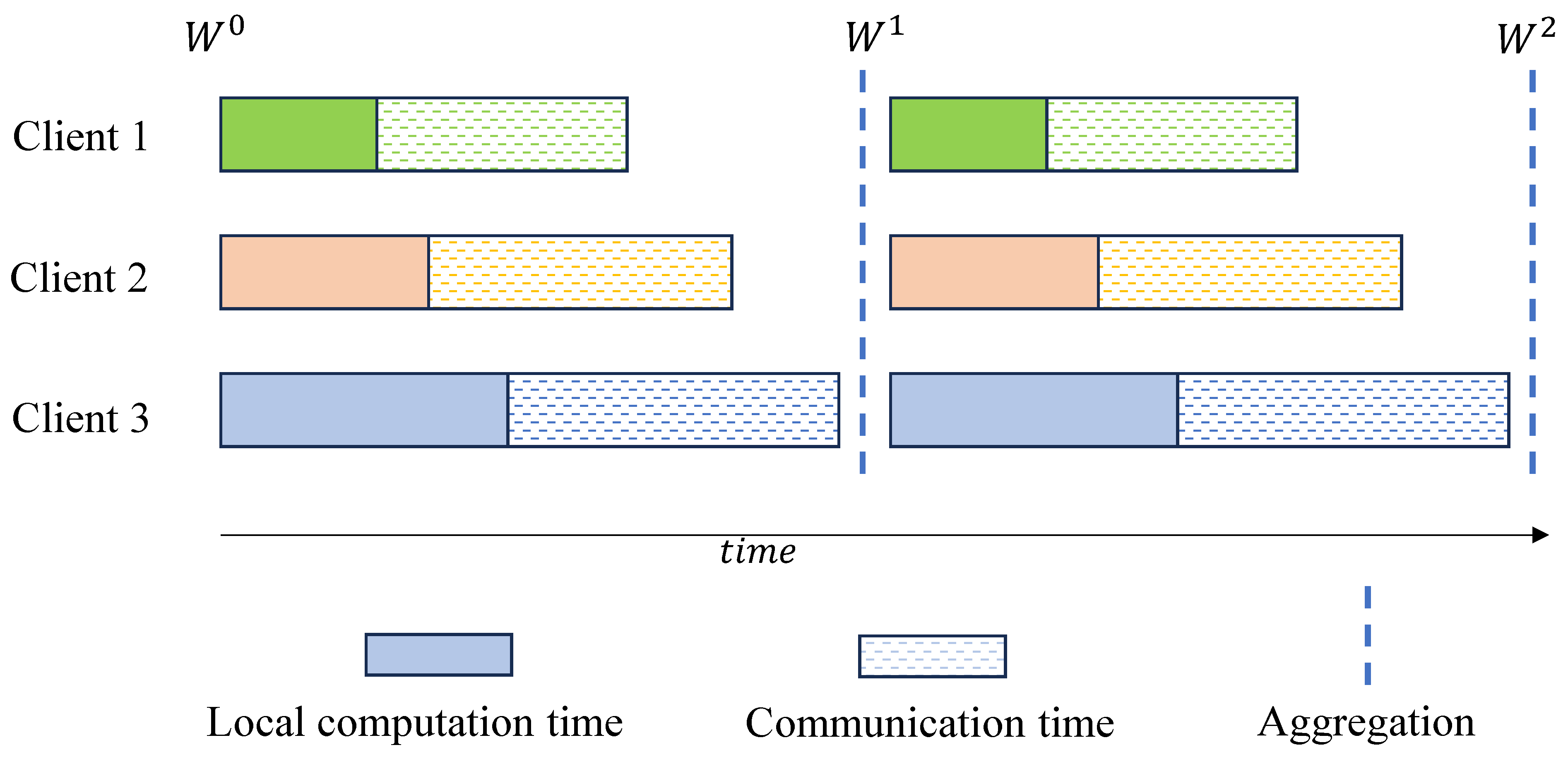
In the training process of wireless FL, a significant portion of the system’s time consumption comes from communication overhead, while the local computation time of clients generally accounts for only about one-tenth of the communication time. Figure 1 shows the synchronous FL training process of three clients. Starting training at the same time, due to the considerable differences in computing capability among the clients, when using the same size data samples for training, clients with higher computing capability (such as Client 1) complete the training first, while clients with weaker computing capability (such as Clients 2 and 3) lag behind. Since each client occupies the same proportion of bandwidth exclusively, the communication time with the edge after completing local training is equal. In this case, high-computing-capability clients send their local models to the edge first, but the edge needs to wait to collect local models sent by all clients before aggregation. Hence, high-computing-capability clients (such as Clients 1 and 2) experience some waiting time. Although this does not impact the overall delay in a single round, if this phenomenon is scaled to all rounds globally and with a large number of clients sharing limited bandwidth, it inevitably results in a significant amount of time wasted.

4. Client–Edge Pairing Based on Similarity and Heterogeneous Computing Capabilities

A way to pair clients and edges based on model similarity is detailed in [15] without considering heterogeneity of clients. However, when there are significant differences in client computing capabilities, this method has drawbacks: although the paired clients under each edge maintain dissimilar data distributions, their computing capabilities may vary greatly. If a synchronous aggregation strategy is maintained, high-computing-capability clients wait for low-computing-capability clients, resulting in extremely long waiting times [16]. Therefore, this section proposes to consider heterogeneous computing capabilities in the pairing method, ensuring that the paired clients under each edge maintain dissimilar data distributions and similar computing capabilities. The specific improvement method is as follows.

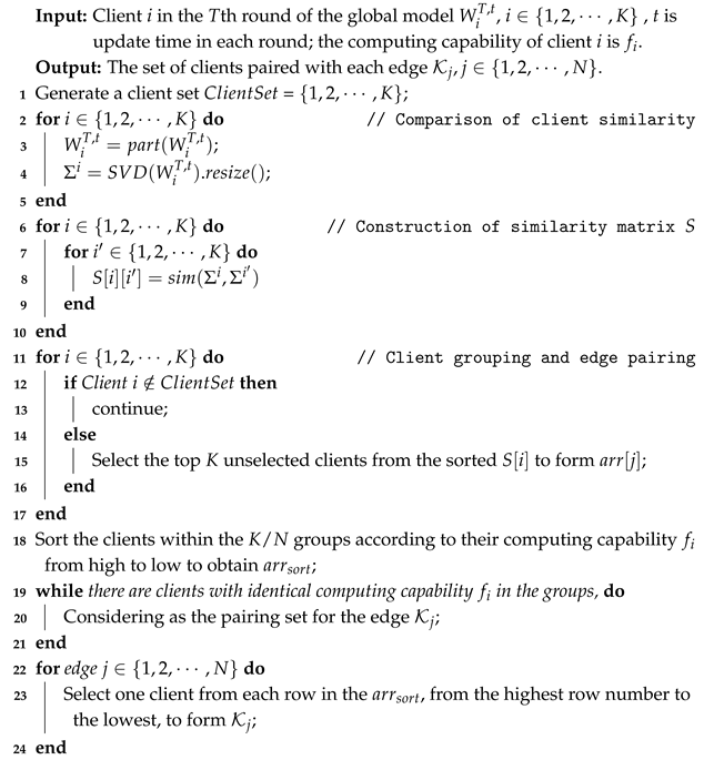
First, we construct a similarity matrix S and group the similarities into $K/N$ groups so that the data distribution characteristics of the clients within each group are approximately similar. Next, we introduce the consideration of heterogeneous computing capabilities: since there are significant differences in computing capabilities among clients within each group, we sort the computing capabilities within each group to obtain the sorted groups. Finally, when the cloud pairs each edge, if there are clients with the same computing capability in each group, they naturally cluster and form a pair for one of the edges. If there are no clients with exactly the same computing capability between groups or if partial matching has been completed, the remaining unselected clients are paired by the edge according to the sorted computing capability, from high to low, based on the sorted row numbers. The specific method is given in Algorithm 1. The paired clients under each edge maintain dissimilar data distributions but similar computing capabilities.

Algorithm 1: Client–edge pairing based on similarity and heterogeneous computing capabilities

The proposed client–edge pairing algorithm acts as a pre-processing module in the training process of a three-tier FL architecture. It performs client grouping based on local model similarity and heterogeneous computing capabilities. Since the algorithm does not directly participate in parameter optimization or model updates, it preserves the convergence properties of standard FL algorithms such as FedAvg or FedProx. By assigning clients with similar model structures to the same edge server, the algorithm reduces intra-group heterogeneity and enhances the quality of local aggregations, thereby improving the stability of global convergence. Moreover, the sorting of clients by computing capability ensures that low-resource devices are only assigned lightweight update tasks, enabling timely synchronization and reducing training latency caused by stragglers.

The computational complexity of Algorithm 1 mainly consists of three parts: singular value decomposition (SVD) of each client’s model, pairwise similarity computation, and client grouping with sorting. We let K denote the number of clients and d the dimensionality of the model parameters. Then, the overall time complexity is $\mathcal{O}\left(K{d}^3+K^{2}d+KlogK\right)$, where $\mathcal{O}\left(K{d}^3\right)$ arises from SVD operations for K clients, $\mathcal{O}\left(K^{2}d\right)$ comes from computing pairwise similarities, and $\mathcal{O}\left(KlogK\right)$ results from sorting clients based on their computing capabilities. In practice, the computational cost can be reduced by employing low-rank approximations or truncated SVD, which significantly speeds up the feature extraction step and enhances scalability for large-scale deployments.

5. Enforced Synchronization Strategy Based on Model Dropout

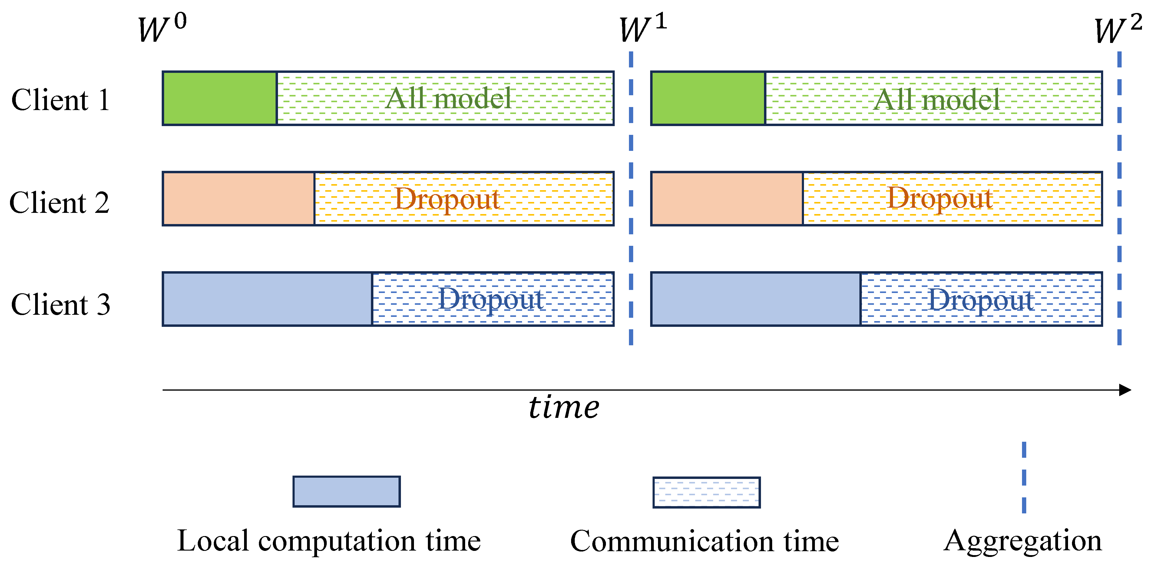
In the previous section, we re-paired the clients based on model similarity and computing capabilities. Although the computing capabilities of clients under the same edge are similar, they are not identical, resulting in some waiting time. This section proposes an enforced synchronization method based on model dropout for client transmissions. Clients with higher computing capability can transmit the entire model, while clients with lower computing capability perform dropout operations on the model using the algorithm in this section, ensuring that all clients’ local models reach the edge simultaneously, as shown in Figure 2.

As a regularization technique, dropout was first introduced in neural network methods to prevent overfitting by making some neurons’ activation values stop working with a certain probability during forward propagation. This prevents the model from relying too heavily on local features and thus improves model generalization [17]. In this section, a fixed proportion of neuron values are set to zero to reduce the pressure and delay of model transmission. We assume that all edges can beforehand know the computing capabilities of each client. Taking a specific edge as an example, when clients complete local updates, if all clients have equal computing capabilities, the entire model can be directly transmitted. If the computing capabilities are unequal, the client with the highest computing capability is used as the baseline. Since each client is allocated equal bandwidth, the time to transmit the entire model is equal, denoted as $T^{cmp}$. The dropout proportion $q_i^M$ for each client’s model can be obtained using the following formula:

$$q_i^M={\displaystyle \frac{T_i^{\mathrm{com}}}{T_{*}^{\mathrm{com}}}}=1-{\displaystyle \frac{T_i^{\mathrm{cmp}}-T_{*}^{\mathrm{cmp}}}{T_{*}^{\mathrm{com}}}}$$

(1)

where $T_{*}^{com}$ and $T_{*}^{cmp}$ represent the time required for the client with the highest computing capability under that edge to perform local updates and model transmission, respectively. To ensure the effectiveness of this method, it is necessary to guarantee that $q_i^M\in (0,1]$. Therefore, the number of local updates needs to be controlled within a reasonable range to avoid the situation where $T_i^{cmp}>T_{*}^{com}+T_{*}^{cmp}$.

When clients transmit model parameters to the edge, they follow the agreed-upon protocol using the dropout proportion $q_i^M$ calculated by Equation (1) to apply dropout to the local model parameters before retransmitting. This selection of dropout parameters is referred to as the mask $M_i^{T,t}$. The generation of this mask can achieve an approximately pseudo-random effect based on some client identifier (such as version number or timestamp of the sent model). In the mask, the parameters to be sent are set to one and those not to be sent are set to zero, with the same dimensions as the model. This work employs lightweight identifiers—such as random seeds or hash signatures—instead of explicitly transmitting masks. Edge nodes can reconstruct the corresponding masks based on the client identifiers and use them to complete the missing portions of the uploaded model parameters. Bandwidth estimation indicates that the overhead introduced by this mechanism constitutes only a minimal fraction of the total uplink data volume, making its transmission latency negligible on typical IoT devices. The completed client model parameters ${\tilde{W}}_{loca{l}_i}^{T,t}$ are

$${\tilde{W}}_{{\mathrm{local}}_i}^{T,t}\leftarrow W_{{\mathrm{local}}_i}^{T,t}\odot M_i^{T,t}+\nu ·W_{{\mathrm{edge}}_j}^{T,t-1}\odot {\left(M_i^{T,t}\right)}^c$$

(2)

where ${\left(M_i^{T,t}\right)}^c$ denotes the complement of the mask; ⊙ denotes the Hadamard product between matrices; the unsent model parameters are replaced with the previous round’s edge model $W_{edg{e}_j}^{T,t-1}$. The proportion is controlled by the hyper-parameter $\nu \in [0,1]$. Once the edge reconstructs all clients’ local models, it can proceed with synchronous aggregation.

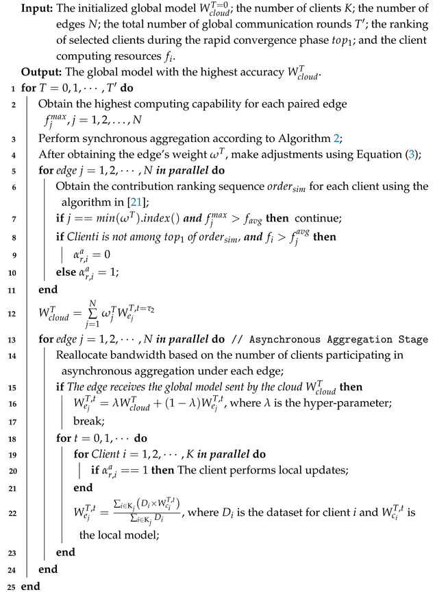
The proposed enforced synchronization strategy based on model dropout, as described in Algorithm 2, is designed to mitigate the impact of heterogeneous computing capabilities among terminal clients in a three-tier FL architecture. By selectively transmitting masked sub-models and enforcing synchronous local updates, the algorithm ensures that all clients—regardless of computing capacity—complete their updates within a fixed number of iterations, thereby aligning their upload timings to the edge servers. This structured synchronization, together with dropout-based model reconstruction at the edge level, enhances the consistency of aggregation and reduces the staleness of updates. Consequently, the method improves convergence stability and ensures the contribution of weak clients without degrading the global model quality. When built upon convergent federated optimization algorithms such as FedAvg, this strategy preserves theoretical convergence while empirically accelerating the training process by reducing idle waiting time and minimizing gradient variance during aggregation.

The computational complexity of Algorithm 2 can be broken down as follows. Each client performs ${\tau }_1$ local updates on a partial model of size $\alpha d$, where d is the dimensionality of the global model and $\alpha$ in (0, 1] is the dropout ratio. The local update cost is thus $\mathcal{O}\left({\tau }_1\alpha d\right)$. Dropout masking and identifier encoding incur negligible overhead. Each edge server reconstructs $K/N$ masked models per round, with a reconstruction cost of $\mathcal{O}\left(\alpha d\right)$ per model. Aggregation and weighting involve an additional $\mathcal{O}\left(Kd\right)$ across all edges. The total complexity per round is $\mathcal{O}\left(K{\tau }_1\alpha d+K\alpha d+Nd\right)$, which is significantly lower than full-model synchronous updates. Moreover, the model compression via dropout reduces communication cost and training latency, making the algorithm well-suited for resource-constrained edge environments.

Algorithm 2: Enforced Synchronization Strategy Based on Model dropout [18]

6. Contribution-Based Aggregation Strategy Optimization Based on Heterogeneous Computing Capabilities

A high-contribution edge model essentially reflects the characteristics of the local dataset more effectively. In homogeneous client scenarios [19], since each client performs the same number of computations, the SV can directly reflect the importance of the dataset to the global model. However, when clients have different computing capabilities and can perform different numbers of local training iterations, directly using the SV as a measure of contribution is inappropriate, as it violates the principle of collaborative fairness in FL. Therefore, this section aims to design a contribution-based aggregation optimization strategy.

In the previous section, we grouped clients with similar computing capabilities into clusters, ensuring that the clients paired with each edge have similar computing capability. Through the dropout method, we also maintained consistent local iteration counts within each cluster, although the iteration counts differ between clusters. If we directly use the SV as the consideration for contribution weight, it may result in a loss of global model accuracy due to insufficient computing capability from originally high-contributing clients. Therefore, this section introduces a reward–punishment mechanism into the weights. 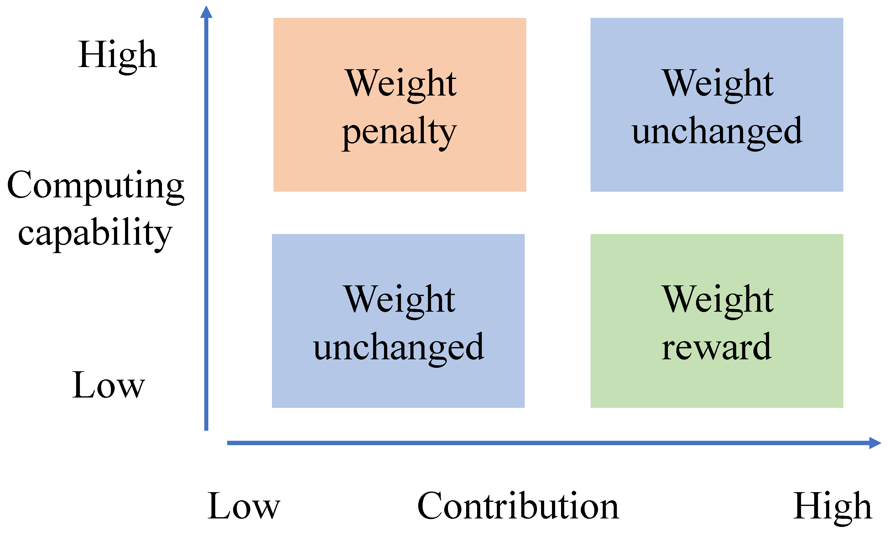Figure 3 presents a quadrant chart, where the horizontal axis represents client contribution and the vertical axis represents client computing resources. By calculating the contribution within each cluster (i.e., SV) and the average computing capability of each cluster, we can influence the weights. The specific explanation is as follows.

Clients within clusters with lower average computing capability have performed fewer local iterations compared to those with higher computing capability; thus, their local models should be less effective at feature extraction. Similarly, clients within clusters with higher average computing capability have performed more iterations and should have better feature extraction capabilities. Therefore, in the upper left and lower right quadrants of the quadrant chart, the SV can be directly used as a weight reference without any rewards or penalties. However, if a cluster with lower average computing capability has an SV higher than the average SV, it indicates that the local data within that cluster are of higher quality and better represents the global model. Thus, a reward factor ${\chi }_i$ (corresponding to the upper right quadrant in the chart) can be introduced to increase the proportion of this edge model in the subsequent weighting, thereby tilting the global model towards this edge model. Conversely, if a cluster with higher average computing capability has an SV lower than the average SV, it is the least desirable situation. It implies that the local data under high-computing-capability clients are of lower quality, offering limited features for the model to learn from. Thus, a penalty factor ${\xi }_i$ (corresponding to the lower left quadrant in the chart) can be introduced to decrease the proportion of this edge model in the subsequent weighting, causing the global model to slightly diverge from this edge model.

Note that this method is limited to appropriate adjustments of SV. If the reward and penalty factors are too large, it may lead to overcorrection, making it difficult for the global model to converge. After analyzing the rewards and penalties for each edge model, we can start optimizing the aggregation weights with the following formula:

$${\omega }_i^T=\left\{\begin{array}{c}{\displaystyle \frac{{\chi }_i{\xi }_{i}as{v}_i}{{\sum }_{i=0,as{v}_i\ge 0}^{i=K}{\chi }_i{\xi }_{i}as{v}_i}},as{v}_i\ge 0,\hfill \\ 0,as{v}_i<0.\hfill \end{array}\right.$$

(3)

where $as{v}_i$ is accumulative SV for client i. If no rewards or penalties are applied to the model, then ${\chi }_i$ and ${\xi }_i$ are both 1.

7. IoT Wireless Resource Allocation Scheme

When clients are homogeneous, it is sufficient to reduce the participation of low-contribution clients in aggregation, thereby allocating more bandwidth resources to high-contribution clients. This allows for more local training to reduce the edge’s local loss function, thereby influencing the global average loss function. However, when clients are heterogeneous, it is necessary to consider that high-contribution clients may consume significant energy and take longer computation times during local calculations. This means they cannot perform multiple iterations within the same energy consumption or time frame. Therefore, this section comprehensively considers contribution and heterogeneous computing capability, selecting clients and allocating bandwidth resources based on the principle of fairness.

The main idea is to optimize client selection within a given time frame during the asynchronous aggregation phase. Specifically, this involves adjusting whether each client i participates in the asynchronous aggregation during the rth round of global aggregation, denoted as ${\alpha }_{r,i}^a$. From a fairness perspective, the contribution of edges and clients (obtained by calculating the Shapley Value (SV) or model similarity) within the same number of training and aggregation cycles can directly reflect data quality [20]. According to the approach from the previous section, edges or clients with higher computing capability should inherently possess stronger data feature extraction capabilities, while those with lower computing capability should be given some tolerance in terms of model performance.

In the specific algorithm, this is reflected as follows: when it is necessary to exclude an edge with a low SV, the maximum computing resource $f_j^{max}$ of the clients under that edge must be considered (since the number of local training iterations after dropout depends on the maximum computing capability under the edge). If $f_j^{max}$ ranks low among all computing capabilitys, it is considered tolerable and is not excluded; however, if $f_j^{max}$ ranks high, it is considered intolerable and can be excluded. Similarly, when using model similarity to assess client contribution and selecting the top clients, the computing capability $f_i$ of clients under each edge needs to be sorted from high to low. If a client has low contribution and ranks low in computing capability, it is considered tolerable, as its data have not been reasonably utilized due to limited computing resources. By allocating more bandwidth resources and training opportunities to it, its model contribution can be improved. Conversely, if a client has low contribution but ranks high in computing capability, it indicates that its local data quality is low. Even with high computing capability, its contribution to the global model is minimal and it is considered intolerable, thus excluded from the client selection strategy. Algorithm 3 provides a detailed explanation using the rapid convergence phase as an example, with the same logic applying to the performance enhancement phase.

In each round, client computation (local updates) for selected participants is $\mathcal{O}\left(K_s{\tau }_{1}d\right)$, where $K_s$ is the number of participating clients. Contribution ranking and participation decision per edge costs $\mathcal{O}(KlogK)$, assuming sorted ranking. Bandwidth reallocation and edge-level aggregation per edge is $\mathcal{O}\left(K_{j}d\right)$, with $K_j$ clients under edge j. Thus, the overall complexity per round is $\mathcal{O}\left(K_s{\tau }_{1}d+NKlogK+N{K}_{j}d\right)$, which scales efficiently due to selective update and avoids full participation overhead. Additionally, the ranking mechanism filters out high-delay or low-impact clients, reducing unnecessary gradient computation and improving resource utilization.

Although Algorithm 3 involves several decision layers to jointly optimize fairness, efficiency, and resource utilization, its modular structure allows for adaptation in practice. For instance, the prioritization step could be replaced by a heuristic rule or sorted by lightweight metrics such as historical reliability or compute availability. While the current design aims to demonstrate the theoretical upper-bound of achievable performance, further simplification tailored to specific deployment contexts is a promising direction for future research.

Algorithm 3: IoT Wireless Resource Allocation Algorithm [21]

8. Simulations

8.1. Simulation Settings

The FL architecture consists of one cloud server, six edge servers, and thirty clients. The system latency primarily comprises three components: first, the computation delay incurred by local training on the client devices and the transmission delay associated with uploading local models; second, the latency at the edge servers, including the time required for edge aggregation, as well as the transmission delay for distributing the aggregated edge models to clients and uploading them to the cloud server; and finally, the latency at the cloud server for performing global aggregation and distributing the global model back to the edge servers. The specific calculation method follows the approach in [22], and the wireless network parameters used in our experiments are listed in

Table 1. Wireless Network Scenario Parameter Settings.

Parameter	Value
Computation cycles per bit $c_i$	30 cycles/bit
Capacitance coefficient $a_i/2$	$2\times {10}^{-26}$
Bandwidth B	$1\times {10}^6$ Hz
Client transmit power $p_i$	0.5 W
Channel gain $h_i$	$1\times {10}^{-8}$
Power spectral density of noise $N_0$	$1\times {10}^{-10}$ W

.

The experiments are conducted on the MNIST [23], CIFAR10 [24], and FashionMNIST [25] datasets, with the target accuracy set to 90% for the MNIST and 80% for the other two datasets. Each client is allocated different computing capability, specifically CPU frequencies $f_i$, randomly assigned from the range $[5,10,15,20]\times {10}^8$. Due to heterogeneity of clients, both synchronous and asynchronous aggregation strategies need to be adjusted. The number of synchronous aggregations for each edge and client is fixed at 2, and the number of asynchronous aggregations at 8. The number of local training iterations for clients paired under each edge is no longer fixed but is determined by the client with the highest computing capability, calculated based on the fixed number of aggregations. 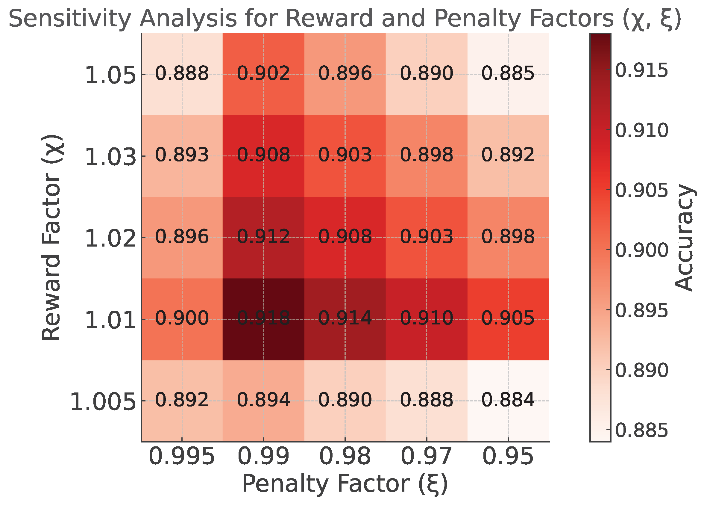To avoid introducing additional delays, the synchronous aggregation time is controlled to be less than the time taken by a client with computing capability $f=1\times {10}^9$ to perform 10 local training iterations as a baseline. The time for asynchronous aggregation should not exceed the communication time between the edge and the cloud. 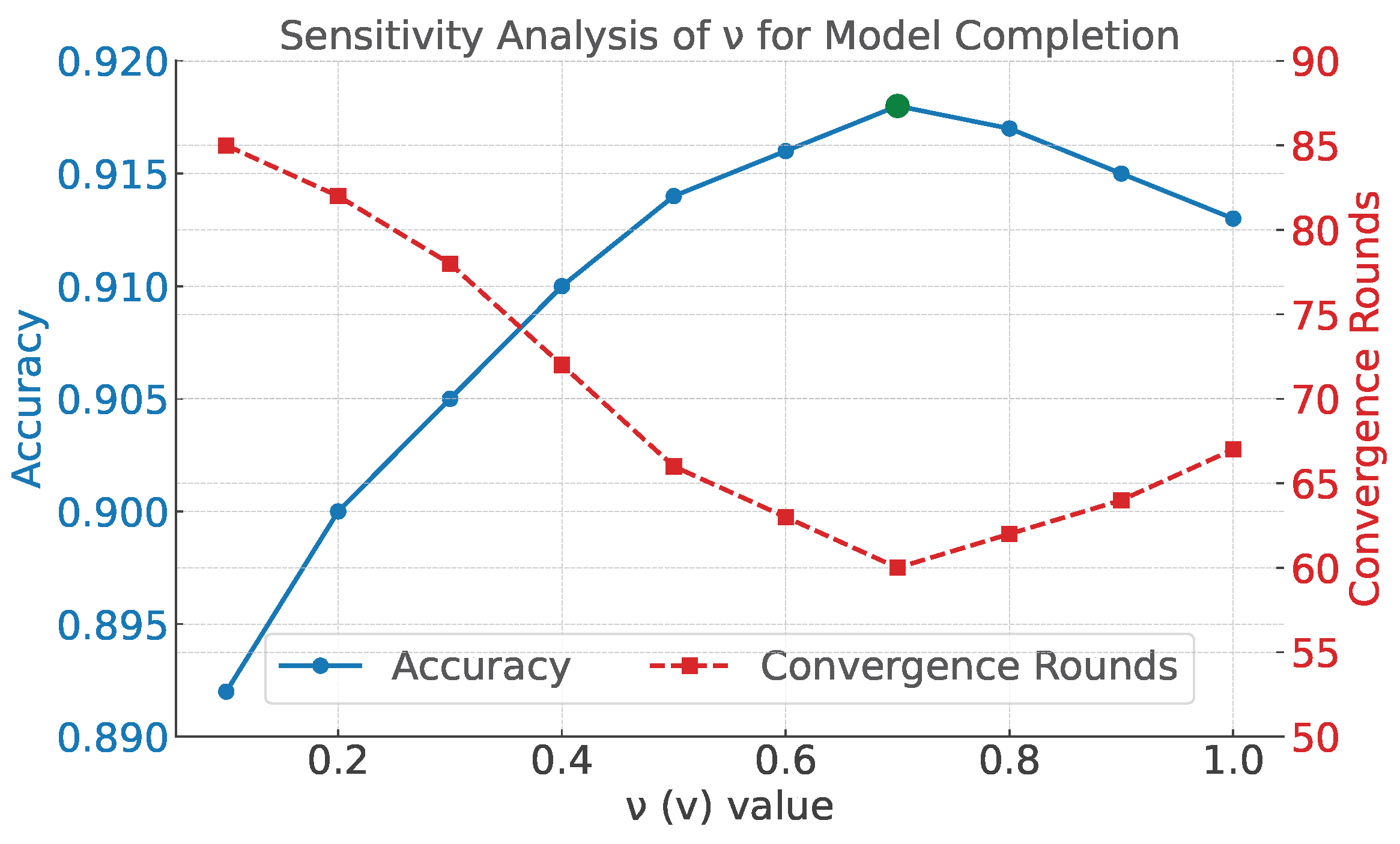The reward and penalty factors for the aggregation weights, ${\chi }_i$ and ${\xi }_i$, are set to 1.01 and 0.99, respectively. The hyperparameter $\nu$ is set to 0.7 in Equation (2). The corresponding sensitivity analysis is provided in Appendix A.

The simulation tests the performance of different resource allocation schemes. The considered metrics are divided into energy consumption targets and accuracy targets: the energy consumption target is the system delay and total client energy consumption when the global model reaches the target accuracy, while the accuracy target is the highest accuracy the global model can achieve after 100 global rounds.

The comparison is primarily made with the following methods:

(1) Method 1: Full aggregation. All clients participate in the aggregation, corresponding to the experimental results from the previous section.

(2) Method 2: Random selection for aggregation. All clients randomly participate in the aggregation according to a fixed proportion frac.

(3) Method 3: Selection of only high-computing capability clients. Clients are selected for aggregation based on their computing capability, according to a fixed proportion frac.

(4) Method 4: Selection of only clients with high local loss [26]. Clients with higher local loss are preferentially selected for aggregation according to the fixed proportion frac.

(5) Method 5: Selection of only high-contribution clients [27].

(6) Method 6: Selection of clients based on a comprehensive evaluation of location, historical information, data characteristics, and current status [22].

The proportion frac is uniformly set to 0.75.

8.2. Simulation Results

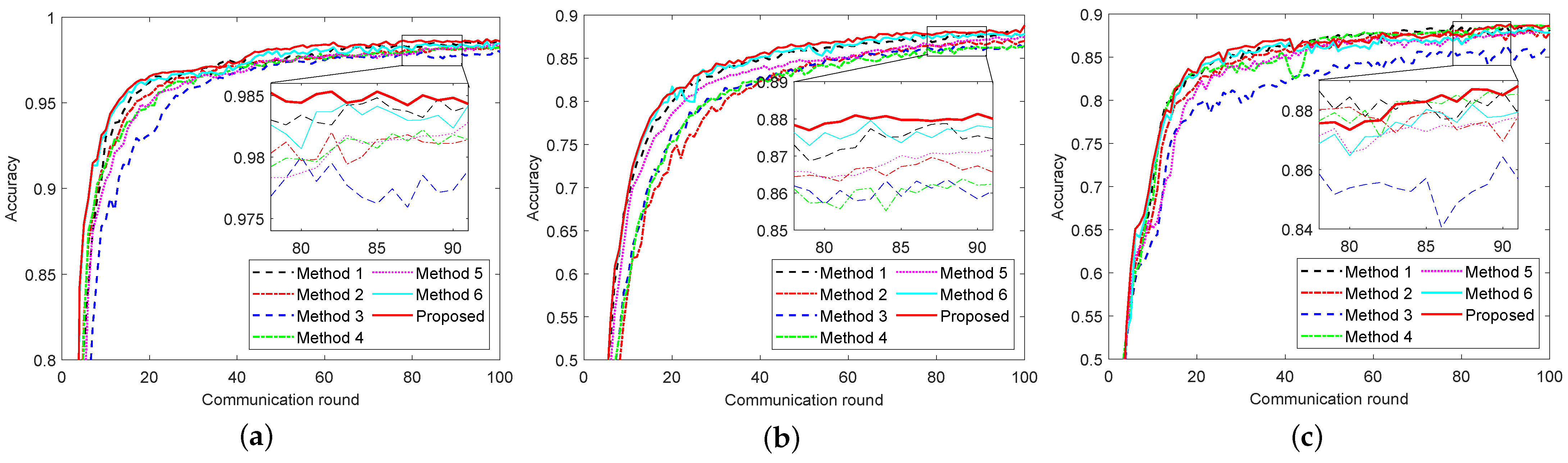
Figure 4 presents the impact curves of different resource allocation methods on the global model across three datasets in a heterogeneous client scenario. Among these methods, Method 3 performs the worst. This method fixes the selected clients during the asynchronous aggregation phase, preventing other clients from participating. As a result, only updates from high-computing-capability clients are received during each aggregation, which harms collaboration fairness and hinders global model updates. Method 2, which employs random selection for aggregation, performs moderately as it can gather information from different clients during the asynchronous aggregation phase. Method 1, which uses a full aggregation strategy, shows better results. Although it gathers more client information, it fails to distinguish the contribution levels of each client, and the number of training iterations per client is lower compared to strategies that involve client selection. Consequently, while Method 1 leads in accuracy, the total energy consumption of the clients remains high. Method 4 measures contribution based on each client’s loss value. This method performs well in later stages, achieving higher global model accuracy. Method 5, designed for client selection in homogeneous client scenarios, saves bandwidth resources, allowing some clients more training opportunities. It also achieves high global model accuracy in later stages. However, since it does not account for heterogeneous computing capability and only relies on SV and model similarity for selection, it loses some truly high-quality clients, leading to delays and higher energy consumption in the early stages, failing to outperform other algorithms. The algorithm proposed in this paper combines the advantages of the above baselines, achieving convergence to a high-performance global model while also ensuring low delay and energy consumption for short-term goals. We also compared it with another federated learning strategy, namely Method 6. Although this approach adopts a multi-criteria client selection scheme, its bandwidth allocation is static, the aggregation strategy relies on the standard FedAvg algorithm, and the fault-tolerance mechanism is based on a fixed participation threshold. As a result, its performance is inferior to the method proposed in this paper. Specific experimental data can be found in

Table 2. System delay and total client energy consumption to achieve the target accuracy under different IoT resource allocation schemes. The “-” indicates that the target accuracy was not reached. TD is time delay (ms), EC is energy consumption (mj). The highest accuracy refers to the maximum accuracy the global model can achieve after 100 rounds of global communication.

MNIST
	Target Accuracy—95%		Target Accuracy—96%		Target Accuracy—97%		Target Accuracy—98%		Highest Accuracy
	TD	EC	TD	EC	TD	EC	TD	EC
Method 1	164	1343	211	1819	444	3462	748	6435	0.9859
Method 2	182	1239	276	1962	453	3099	981	6954	0.9828
Method 3	296	1632	371	2138	569	3423	-	-	0.9808
Method 4	255	1514	291	1738	509	2991	1034	6279	0.9827
Method 5	212	1427	315	2182	518	3549	979	7028	0.9839
Method 6	177	1122	256	1629	493	3418	831	6315	0.9857
Proposed	139	1046	174	1311	444	3307	627	5085	0.9865
CIFAR10
	Target Accuracy—80%		Target Accuracy—85%		Target Accuracy—87%		Target Accuracy—88%		Highest Accuracy
	TD	EC	TD	EC	TD	EC	TD	EC
Method 1	33,003	302,417	77,411	720,087	132,883	1,233,245	179,835	1,668,598	0.8808
Method 2	56,067	425,742	101,316	771,132	178,139	1,363,374	-	-	0.8707
Method 3	50,954	340,572	96,168	660,553	-	-	-	-	0.8635
Method 4	50,973	340,210	134,439	787,462	-	-	-	-	0.8613
Method 5	42,411	286,778	101,314	674,537	159,341	1,078,677	-	-	0.8710
Method 6	38,169	271,664	95,652	643,017	1,612,855	1,065,241	153,328	1,459,732	0.8804
Proposed	27,911	252,493	66,315	601,482	108,145	972,479	131,176	1,123,961	0.8843
FashionMNIST
	Target Accuracy—80%		Target Accuracy—85%		Target Accuracy—87%		Target Accuracy—88%		Highest Accuracy
	TD	EC	TD	EC	TD	EC	TD	EC
Method 1	2769	25,256	6001	54,454	10,464	96,068	14,934	137,331	0.8865
Method 2	3486	25,879	6626	49,244	11,516	86,231	17,402	130,443	0.8811
Method 3	4628	30,206	14,933	97,586	-	-	-	-	0.8643
Method 4	2733	16,555	8287	53,243	10,661	70,713	17,425	121,775	0.8866
Method 5	3622	22,117	8082	52,604	12,336	87,948	21,874	123,523	0.8805
Method 6	3018	20,414	6910	44,146	10,115	80,912	19,989	122,671	0.8857
Proposed	2665	18,220	4763	33,071	8295	58,221	17,431	120,782	0.8882

.

The IoT wireless resource allocation scheme proposed in this paper comprehensively considers the heterogeneous computing capabilities of clients and the contribution of their models, avoiding the neglect of truly high-contribution clients in simple selection methods. From the perspective of energy consumption, the system delay and energy consumption required to achieve the specified accuracy are significantly reduced, with up to 70% of the time saved in reaching the target and up to 60% of client energy consumption conserved. In terms of accuracy, under the same 100 rounds of global communication, this algorithm can further improve the maximum accuracy of the global model by approximately 0.06% to 0.39% compared to not performing client selection (i.e., Method 1).

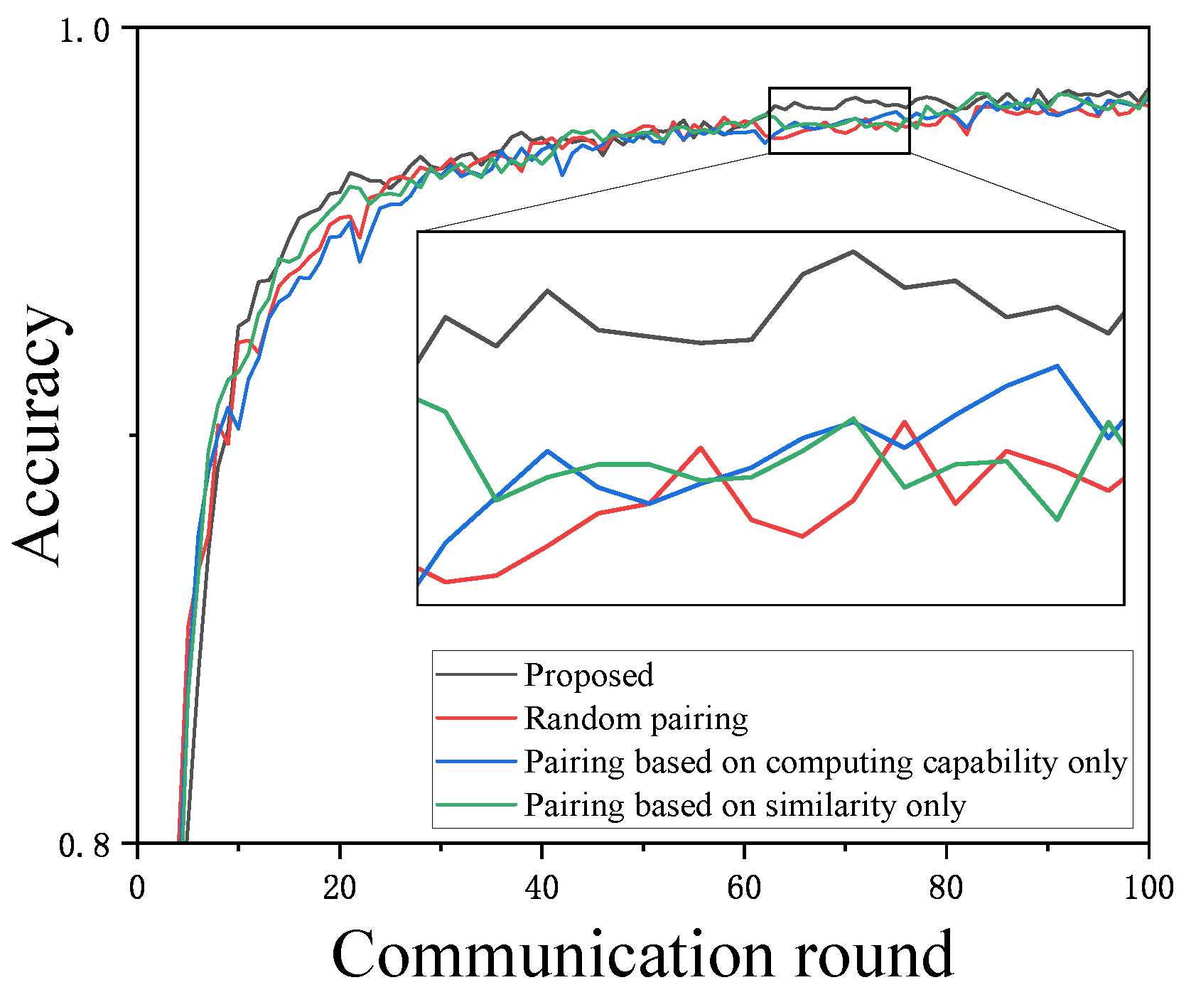
We continue to conduct ablation experiments on two aspects of the proposed scheme: pairing optimization and contribution weight reward–penalty factors. The experiments focus on the performance of the global model in FL, specifically the maximum accuracy within 100 communication rounds and the number of global rounds required to reach the specified accuracy. First, we validate the experimental effect of pairing optimization by comparing it with the following edge-client pairing methods on the MNIST dataset, ensuring that all other conditions remain the same:

(1) Random pairing;

(2) Pairing based on similarity only;

(3) Pairing based on computing capability only, where all clients are sorted by computing capability from highest to lowest, and each edge only considers clients with the same or similar computing capabilities.

Figure 5 shows the impact of different pairing methods on global accuracy. It can be observed that although the differences among the four methods are not significant, there are still subtle variations: pairing based solely on computing capability and random pairing yield the worst results, further confirming the importance of similarity-based pairing within this framework. It also indicates that there is no need to pair clients based solely on computing capability similarity, as the dropout method can approximate this effect. Pairing based solely on similarity can result in significant differences in computing capability within each edge, leading to more model parameter loss when using dropout for enforced synchronization, making it unsuitable for heterogeneous client scenarios. The proposed method outperforms the other three pairing methods.

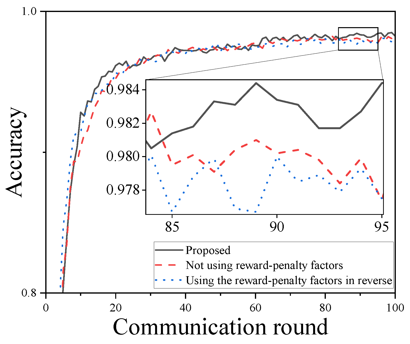
Finally, an ablation experiment is conducted on the reward–penalty factor strategy, primarily comparing the scenarios of not using reward–penalty factors and using the reward–penalty factors in reverse (i.e., swapping ${\chi }_i$ and ${\xi }_i$). The results on the MNIST dataset are shown in Figure 6. It can be observed that the overall effect of using the reward–penalty factors is the best, while the methods of not using them and using them in reverse show slightly worse performance. The reason the method without reward–penalty factors performs slightly worse is that it fails to fully integrate heterogeneous computing capabilities into the contribution evaluation. Without this consideration, the performance is diminished in scenarios with heterogeneous clients.

9. Conclusions

This paper studies communication resource allocation in cloud–edge–client FL under heterogeneous IoT client computing capabilities. We designed an enforced synchronization update strategy based on model dropout, allowing each client to simultaneously transmit model parameters to the edge during each aggregation, combining the advantages of both synchronous and asynchronous methods. We incorporated heterogeneous computing capabilities into the pairing consideration, ensuring that the data samples covered by each edge are dissimilar while maintaining similar computing capability. Additionally, we designed reward–penalty factors to make the proposed method more targeted for scenarios with heterogeneous computing capabilities. Furthermore, the factor of heterogeneous computing capability was also integrated into the client selection and bandwidth allocation algorithms, which, compared to strategies that consider only contribution or computing capability, can further reduce IoT system delay and energy consumption while improving the performance of the final model.