
Balancing Prediction Accuracy and Explanation Power of Path Loss Modeling in a University Campus Environment via Explainable AI


Abstract
1. Introduction
2. Literature Review
3. Data
4. Evaluation Models
4.1. Empirical Models
- (1)
- Okumura–Hata Model
- (2)
- COST-231 Hata Model
- (3)
- ECC-33 Model
4.2. Black Box ML Models
- (1)
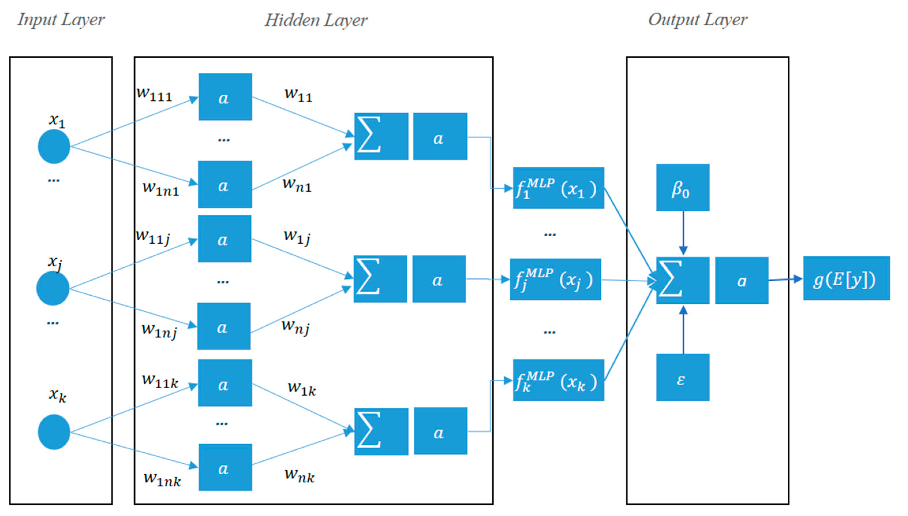
- MLP (multi-layer perception)
- (2)
- XGB (extreme gradient boosting)
- (3)
- RF (random forest)
4.3. Glass Box ML Models
- (1)
- GAM (generalized additive model)
- (2)
- GNAM (generalized neural additive model)
- (3)
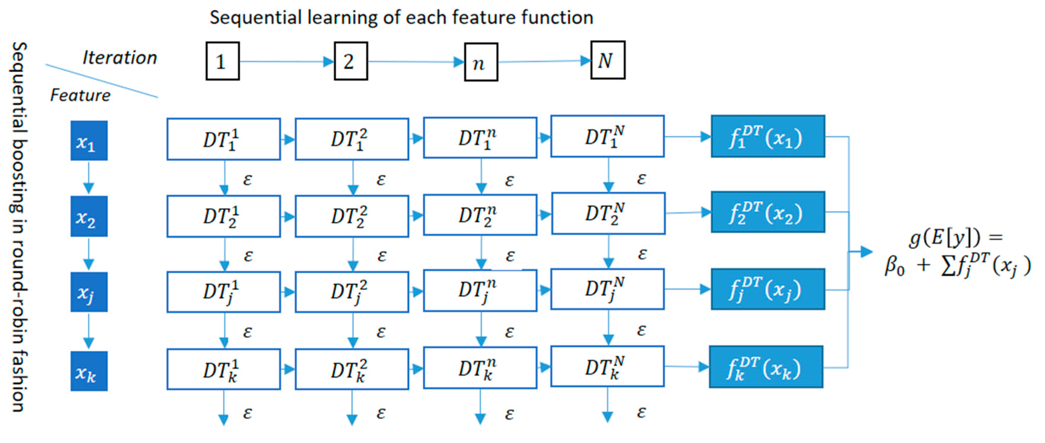
- EBM (explainable boosting machine)
5. Model Accuracy Results
6. Model Interpretation Results
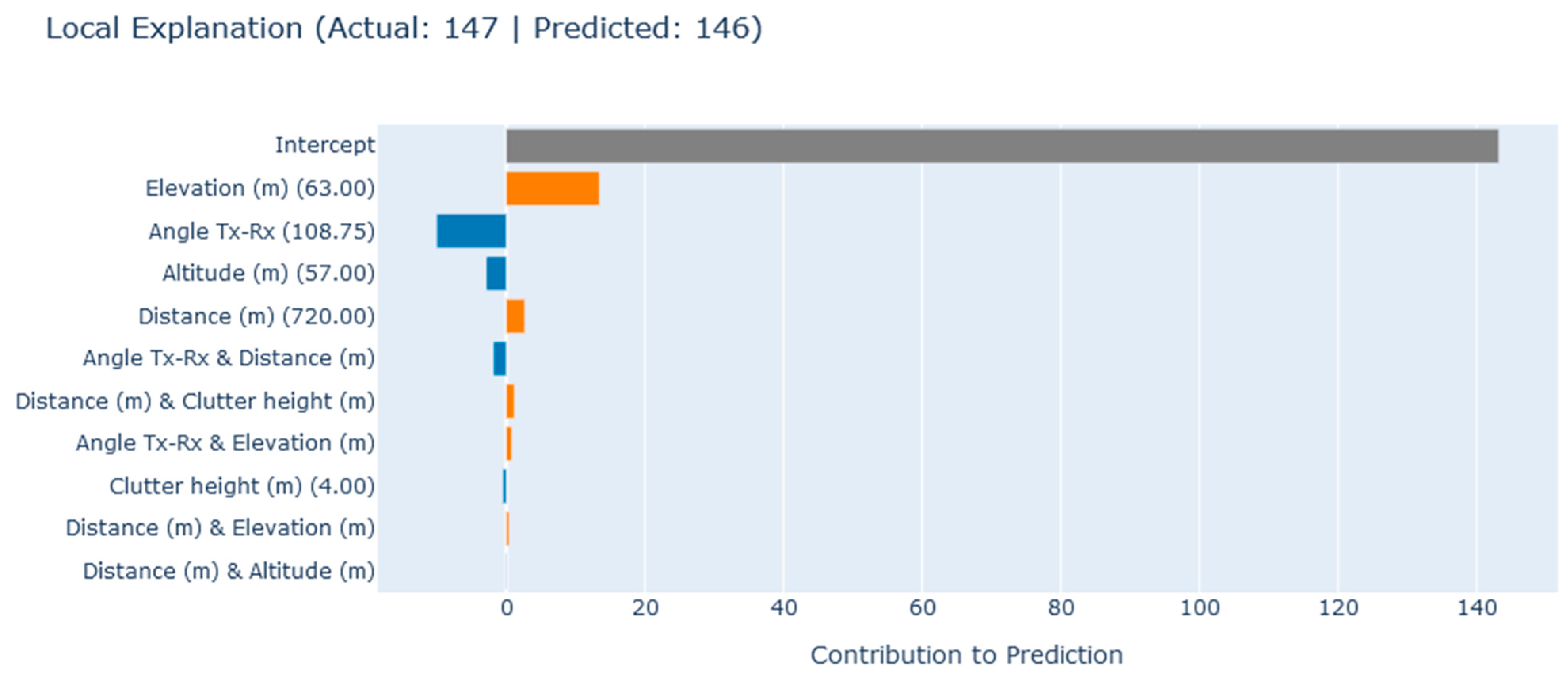
6.1. Local Explanations
6.2. Global Explanations
- (1)
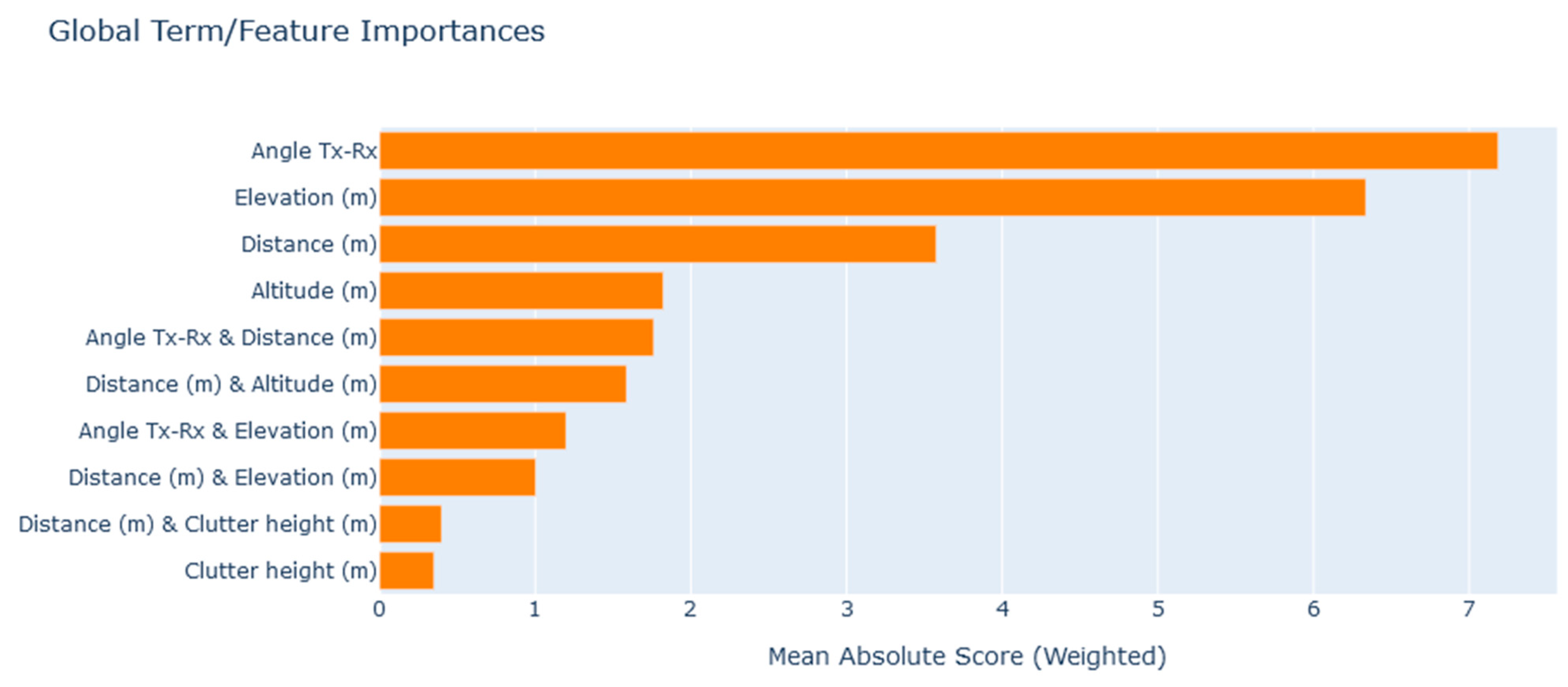
- Feature Significance
- (2)
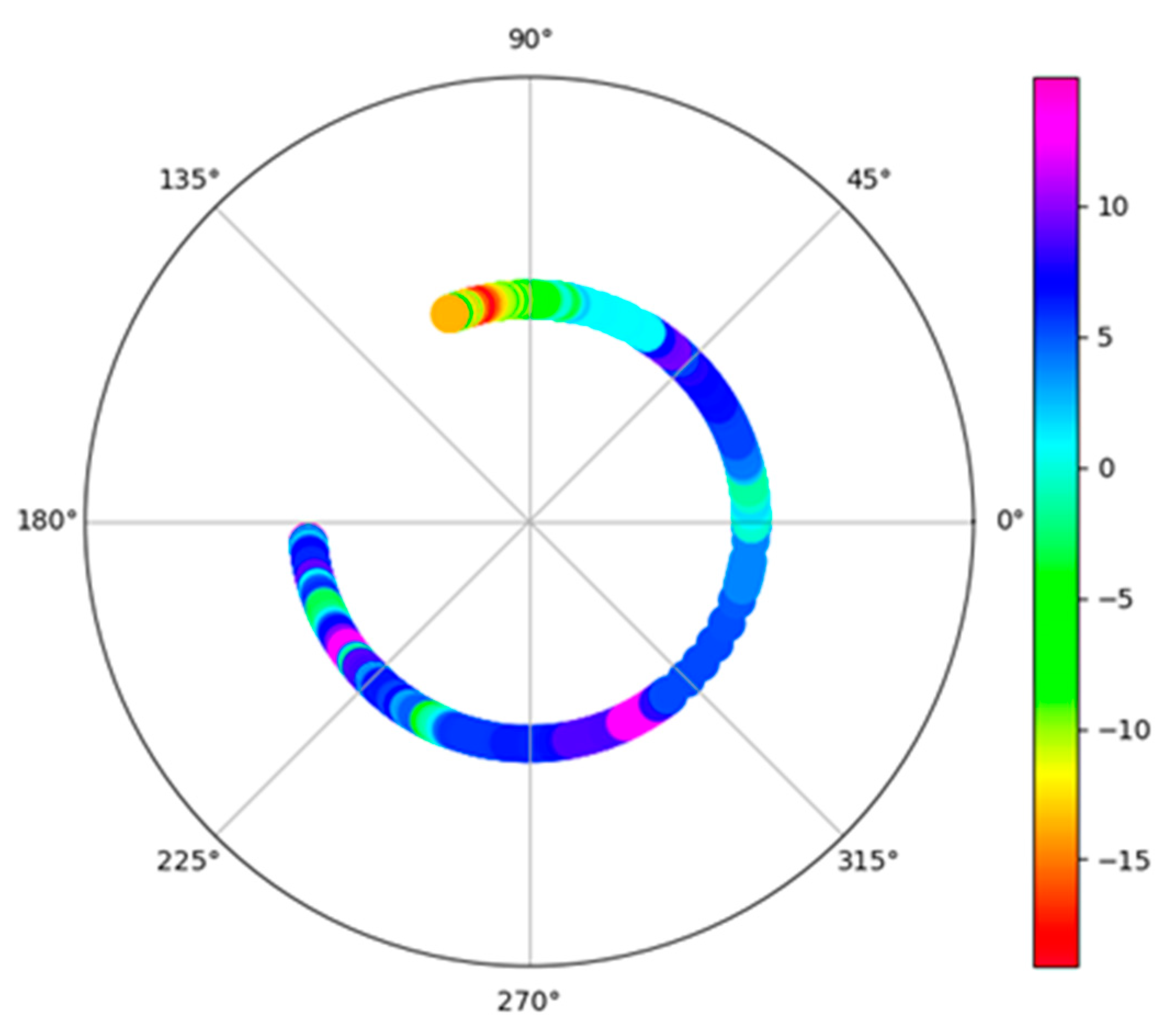
- Feature Marginal Contribution
- (3)
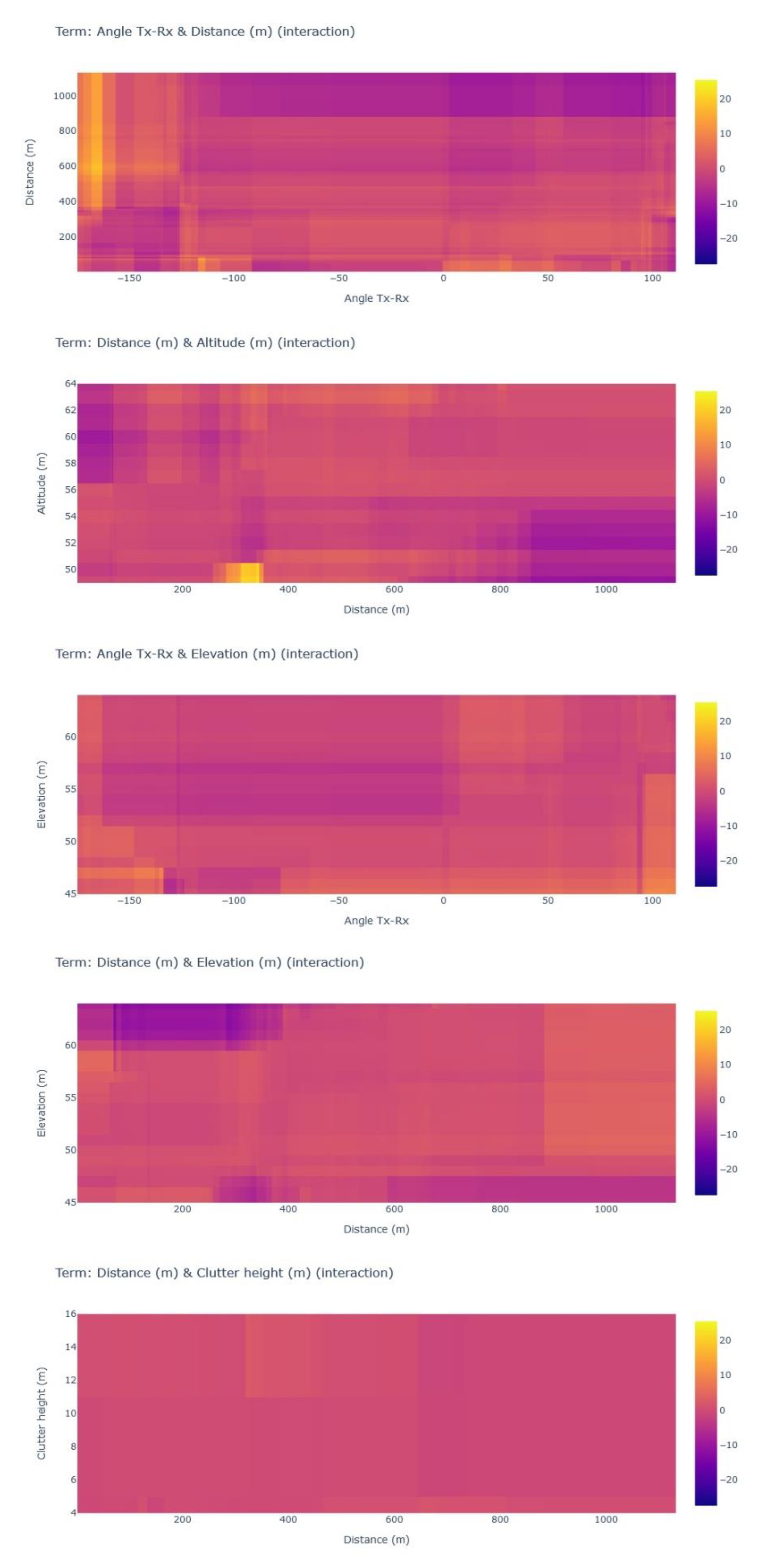
- Interactive Feature Marginal Contribution
7. Conclusions
Supplementary Materials
Author Contributions
Funding
Data Availability Statement
Conflicts of Interest
References
- Khanh, Q.V.; Hoai, N.V.; Manh, L.D.; Le, A.N.; Jeon, G. Wireless Communication Technologies for IoT in 5G: Vision, Applications, and Challenges. Wirel. Commun. Mob. Comput. 2022, 2022, 3229294. [Google Scholar] [CrossRef]
- Phillips, C.; Sicker, D.; Grunwald, D. A survey of wireless path loss prediction and coverage mapping methods. IEEE Commun. Surv. Tutor. 2013, 15, 255–270. [Google Scholar] [CrossRef]
- Shaibu, F.E.; Onwuka, E.N.; Salawu, N.; Oyewobi, S.S.; Djouani, K.; Abu-Mahfouz, A.M. Performance of Path Loss Models over Mid-Band and High-Band Channels for 5G Communication Networks: A Review. Future Internet 2023, 15, 362. [Google Scholar] [CrossRef]
- Miller, T. Explanation in artificial intelligence: Insights from the social sciences. Artif. Intell. 2019, 267, 1–38. [Google Scholar] [CrossRef]
- Allgaier, J.; Mulansky, L.; Draelos, R.L.; Pryss, R. How does the model make predictions? A systematic literature review on the explainability power of machine learning in healthcare. Artif. Intell. Med. 2023, 143, 102616. [Google Scholar] [CrossRef]
- Confalonieri, R.; Coba, L.; Wagner, B.; Besold, T.R. A historical perspective of explainable Artificial Intelligence. WIREs Data Min. Knowl. Discov. 2021, 11, e1391. [Google Scholar] [CrossRef]
- Angelov, P.P.; Soares, E.A.; Jiang, R.; Arnold, N.I.; Atkinson, P.M. Explainable artificial intelligence: An analytical review. WIREs Data Min. Knowl. Discov. 2021, 11, e1424. [Google Scholar] [CrossRef]
- Vollert, S.; Atzmueller, M.; Theissler, A. Interpretable Machine Learning: A brief survey from the predictive maintenance perspective. In Proceedings of the 2021 26th IEEE International Conference on Emerging Technologies and Factory Automation (ETFA), Vasteras, Sweden, 7–10 September 2021; pp. 1–8. [Google Scholar] [CrossRef]
- Popoola, S.I.; Atayero, A.A.; Arausi, Q.D.; Matthews, V.O. Path loss dataset for modeling radio wave propagation in smart campus environment. Data Brief 2018, 17, 1062–1073. [Google Scholar] [CrossRef]
- Popoola, S.I.; Atayero, A.A.; Popoola, O.A. Comparative assessment of data obtained using empirical models for path loss predictions in a university campus environment. Data Brief 2018, 18, 380–393. [Google Scholar] [CrossRef]
- Juang, R.T. Explainable Deep-Learning-Based Path Loss Prediction from Path Profiles in Urban Environments. Appl. Sci. 2021, 11, 6690. [Google Scholar] [CrossRef]
- Yazici, I.; Özkan, E.; Gures, E. Enhancing Path Loss Prediction Through Explainable Machine Learning Approach. In Proceedings of the 2024 11th International Conference on Wireless Networks and Mobile Communications (WINCOM), Leeds, UK, 23–25 July 2024; pp. 1–5. [Google Scholar] [CrossRef]
- Sani, U.S.; Malik, O.A.; Lai, D.T.C. Improving Path Loss Prediction Using Environmental Feature Extraction from Satellite Images: Hand-Crafted vs. Convolutional Neural Network. Appl. Sci. 2022, 12, 7685. [Google Scholar] [CrossRef]
- Nuñez, Y.; Lisandro, L.; da Silva Mello, L.; Orihuela, C. On the interpretability of machine learning regression for path-loss prediction of millimeter-wave links. Expert Syst. Appl. 2023, 215, 119324. [Google Scholar] [CrossRef]
- Sun, Y.; Zhang, Y.; Yu, L.; Yuan, Z.; Liu, G.; Wang, Q. Environment Features-Based Model for Path Loss Prediction. IEEE Wirel. Commun. Lett. 2022, 11, 2010–2014. [Google Scholar] [CrossRef]
- Liao, X.; Zhou, P.; Wang, Y.; Zhang, J. Path Loss Modeling and Environment Features Powered Prediction for Sub-THz Communication. IEEE Open J. Antennas Propag. 2024, 5, 1734–1746. [Google Scholar] [CrossRef]
- Elshennawy, W. Large Intelligent Surface-Assisted Wireless Communication and Path Loss Prediction Model Based on Electromagnetics and Machine Learning Algorithms. Prog. Electromagn. Res. C 2022, 119, 65–79. [Google Scholar] [CrossRef]
- Nuñez, Y.; Lisandro, L.; da Silva Mello, L.; Ramos, G.; Leonor, N.R.; Faria, S.; Caldeirinha, F.S. Path Loss Prediction for Vehicular-to-Infrastructure Communication Using Machine Learning Techniques. In Proceedings of the 2023 IEEE Virtual Conference on Communications (VCC), Virtual, 28–30 November 2023; pp. 270–275. [Google Scholar] [CrossRef]
- Hussain, S.; Bacha, S.F.N.; Cheema, A.A.; Canberk, B.; Duong, T.Q. Geometrical Features Based-mmWave UAV Path Loss Prediction Using Machine Learning for 5G and Beyond. IEEE Open J. Commun. Soc. 2024, 5, 5667–5679. [Google Scholar] [CrossRef]
- Turan, B.; Uyrus, A.; Koc, O.N.; Kar, E.; Coleri, S. Machine Learning Aided Path Loss Estimator and Jammer Detector for Heterogeneous Vehicular Networks. In Proceedings of the 2021 IEEE Global Communications Conference (GLOBECOM), Madrid, Spain, 7–11 December 2021; pp. 1–6. [Google Scholar] [CrossRef]
- Wieland, F.; Drescher, Z.; Houser, J. Comparing Path Loss Prediction Methods for Low Altitude UAS Flights. In Proceedings of the 2021 IEEE/AIAA 40th Digital Avionics Systems Conference (DASC), San Antonio, TX, USA, 3–7 October 2021; pp. 1–7. [Google Scholar] [CrossRef]
- Khalili, H.; Wimmer, M.A. Towards Improved XAI-Based Epidemiological Research into the Next Potential Pandemic. Life 2024, 14, 783. [Google Scholar] [CrossRef]
- Perrier, A. Feature Importance in Random Forests. Cit. on p. 6. 2015. Available online: https://scholar.google.com/scholar?q=Perrier,%20A.%20Feature%20Importance%20in%20Random%20Forests.%20Cit.%20on%20p.%206.%202015 (accessed on 28 February 2025).
- Ahmed, N.S.; Sadiq, M.H. Clarify of the Random Forest Algorithm in an Educational Field. In Proceedings of the 2018 International Conference on Advanced Science and Engineering (ICOASE), Duhok, Iraq, 9–11 October 2018; pp. 179–184. [Google Scholar] [CrossRef]
- Rostami, M.; Oussalah, M.A. Novel explainable COVID-19 diagnosis method by integration of feature selection with random forest. Inform. Med. Unlocked 2022, 30, 100941. [Google Scholar] [CrossRef]
- Sharma, P.; Singh, R.K. Comparative Analysis of Propagation Path loss Models with Field Measured Data. Int. J. Eng. Sci. Technol. 2010, 2, 2008–2013. [Google Scholar]
- Singh, H.; Gupta, S.; Dhawan, C.; Mishra, A. Path Loss Prediction in Smart Campus Environment: Machine Learning-based Approaches. In Proceedings of the 2020 IEEE 91st Vehicular Technology Conference (VTC2020-Spring), Antwerp, Belgium, 25–28 May 2020; pp. 1–5. [Google Scholar] [CrossRef]
- Chen, T.; Guestrin, C. XGBoost: A scalable tree boosting system. In Proceedings of the 22nd ACM SIGKDD International Conference on Knowledge Discovery and Data Mining, San Francisco, CA, USA, 13–17 August 2016; pp. 785–794. [Google Scholar]
- Breiman, L. Random Forests. Mach. Learn. 2001, 45, 5–32. [Google Scholar] [CrossRef]
- Molnar, C. Interpretable Machine Learning. A Guide for Making Black Box Models Explainable. 2022. Available online: https://christophmolnar.com/books/ (accessed on 9 January 2025).
- Hastie, T.J.; Tibshirani, R.J. Generalized Additive Models, 1st ed.; Routledge: London, UK, 2017. [Google Scholar]
- Agarwal, R.; Melnick, L.; Frosst, N.; Zhang, X.; Lengerich, B.; Caruana, R.; Hinton, G. Neural Additive Models: Interpretable Machine Learning with Neural Nets. arXiv 2021, arXiv:2004.13912. [Google Scholar]
- Nori, H.; Jenkins, S.; Koch, P.; Caruana, R. InterpretML: A Unified Framework for Machine Learning Interpretability; Microsoft Corporation: Redmond, WA, USA, 2019; Available online: https://arxiv.org/pdf/1909.09223 (accessed on 9 January 2025).
- Greenwell, B.M.; Dahlmann, A.; Dhoble, S. Explainable Boosting Machines with Sparsity: Maintaining Explainability in High-Dimensional Settings. arXiv 2023, arXiv:2311.07452. [Google Scholar]
- Lou, Y.; Caruana, R.; Gehrke, J.; Hooker, G. Accurate intelligible models with pairwise interactions. In Proceedings of the 19th ACMSIGKDD International Conference on Knowledge Discovery and Data Mining, Chicago, IL, USA, 11–14 August 2013; pp. 623–631. [Google Scholar]


| Database | Search Term | X = Path Loss Y = Explainable | X = Path Loss Y = Interpretable | X = Path Loss Y = Feature Importance | X = Path Loss Y = SHAPley |
|---|---|---|---|---|---|
| IEEE Xplore | (“Document Title”: “X”) AND (“Full Text Only”: “Y”) Filters Applied: 2020–2024 | 5 | 4 | 57 | 4 |
| ScienceDirect | Find articles with these terms “Y” Year: 2020–2024 Title, abstract, keywords: “X” | 23 | 10 | 14 | 1 |
| ACM | [Title: path loss] AND [Full Text: “Y”] AND [Title: “X”] AND [E-Publication Date: (1 January 2020 TO 31 October 2024)] | 4 | 4 | 5 | 0 |
| Google Scholar | intitle:”X” intext:”Y” since 2020 | 21 | 10 | 29 | 7 |
| Paper | Propagation Environment | Model Training Method | Model Interpretation Method |
|---|---|---|---|
| [11] | Urban propagation environments for 5G cellular communication systems | Deep learning | Linear regression (LR) |
| [12] | Millimeter waves for different scenarios, including urban micro and urban macro | Extreme gradient boosting (XGB) | SHAP (Shapley additive explanations) and LIME (local interpretable model-agnostic explanations) |
| [13] | Rural, urban, suburban, and urban high-rise environments with different frequency bands and transmitting antenna heights | XGB + other MLs | SHAP |
| [14] | Indoor environment for 5G millimeter-wave frequencies, from 26.5 to 40 GHz | Artificial neural network (ANN), support vector regression (SVR), random forest (RF), and gradient tree boosting (GTB) | Permutation feature importance (PFI), Accumulated local effect (ALE) |
| [15] | Constructed a dataset with the three-dimensional modeling software Blender and the commercial ray tracing (RT) tool WirelessInSite with a random scattered layout and 6 and 28 GHz frequency bands | RF | SHAP |
| [16] | Measurement campaigns at 220 GHz and 280 GHz, where the scenarios include the hallway, lobby, and laboratory | RF | SHAP |
| [17] | Large intelligent surface-assisted wireless communication in a smart radio environment | RF + other MLs | PFI |
| [18] | Vehicular-to-infrastructure communication systems | ANN, SVR, RF, and GTB | PFI, ALE |
| [19] | UAV-assisted millimeter-wave (mmWave) radio network | LR, SVR, K nearest neighbors (KNN), RF, XGB, and ANN | PFI |
| [20] | Vehicle-to-vehicle (V2V) communication systems | RF | Mean decrease impurity method |
| [21] | Low-altitude UAS flights | RF | Mean decrease impurity method |
| Empirical Models | Black Box ML Models | Glass Box ML Models | |||||||
|---|---|---|---|---|---|---|---|---|---|
| Okumura–Hata | COST 231 | ECC-33 | RF | XGB | MLP | GAM | GNAM | EBM | |
| MAE | 8.478 | 7.073 | 13.451 | 2.541 | 2.415 | 3.554 | 2.579 | 3.447 | 2.263 |
| RMSE | 11.103 | 9.815 | 14.669 | 3.790 | 3.264 | 4.916 | 3.38 | 4.406 | 2.918 |
| R Squared | −0.792 | −0.4 | −2.128 | 0.878 | 0.909 | 0.732 | 0.873 | 0.785 | 0.905 |
| Empirical Models | Black Box ML Models | Glass Box ML Models | |||||||
|---|---|---|---|---|---|---|---|---|---|
| Okumura–Hata | COST 231 | ECC-33 | RF | XGB | MLP | GAM | GNAM | EBM | |
| MAE | 6.980 | 7.009 | 18.881 | 2.666 | 2.694 | 3.636 | 2.957 | 3.650 | 2.369 |
| RMSE | 10.119 | 9.994 | 20.522 | 3.402 | 3.544 | 4.773 | 3.682 | 4.745 | 2.989 |
| R Squared | −0.151 | −0.122 | −3.734 | 0.841 | 0.82 | 0.745 | 0.848 | 0.748 | 0.900 |
| Empirical Models | Black Box ML Models | Glass Box ML Models | |||||||
|---|---|---|---|---|---|---|---|---|---|
| Okumura–Hata | COST 231 | ECC-33 | RF | XGB | MLP | GAM | GNAM | EBM | |
| MAE | 13.792 | 12.862 | 12.393 | 1.885 | 2.116 | 4.408 | 3.077 | 4.058 | 2.315 |
| RMSE | 18.559 | 17.513 | 14.976 | 2.644 | 2.893 | 6.207 | 4.129 | 5.356 | 3.031 |
| R Squared | −6.128 | −5.347 | −3.641 | 0.868 | 0.842 | 0.273 | 0.678 | 0.459 | 0.826 |
Disclaimer/Publisher’s Note: The statements, opinions and data contained in all publications are solely those of the individual author(s) and contributor(s) and not of MDPI and/or the editor(s). MDPI and/or the editor(s) disclaim responsibility for any injury to people or property resulting from any ideas, methods, instructions or products referred to in the content. |
© 2025 by the authors. Licensee MDPI, Basel, Switzerland. This article is an open access article distributed under the terms and conditions of the Creative Commons Attribution (CC BY) license (https://creativecommons.org/licenses/by/4.0/).
Share and Cite
Khalili, H.; Frey, H.; Wimmer, M.A. Balancing Prediction Accuracy and Explanation Power of Path Loss Modeling in a University Campus Environment via Explainable AI. Future Internet 2025, 17, 155. https://doi.org/10.3390/fi17040155
Khalili H, Frey H, Wimmer MA. Balancing Prediction Accuracy and Explanation Power of Path Loss Modeling in a University Campus Environment via Explainable AI. Future Internet. 2025; 17(4):155. https://doi.org/10.3390/fi17040155
Chicago/Turabian StyleKhalili, Hamed, Hannes Frey, and Maria A. Wimmer. 2025. "Balancing Prediction Accuracy and Explanation Power of Path Loss Modeling in a University Campus Environment via Explainable AI" Future Internet 17, no. 4: 155. https://doi.org/10.3390/fi17040155
APA StyleKhalili, H., Frey, H., & Wimmer, M. A. (2025). Balancing Prediction Accuracy and Explanation Power of Path Loss Modeling in a University Campus Environment via Explainable AI. Future Internet, 17(4), 155. https://doi.org/10.3390/fi17040155