Abstract
With the increasing predominance of public cloud computing, managing the cost of usage for end users has become vital in importance. Task scheduling has emerged as an important target of research in this area. The present work considers the problem of assigning tasks with different priorities to clouds, with the main requirement being to ensure the meeting of deadlines for high-priority tasks at all costs. The idea is to use as many public cloud resources as needed to satisfy this constraint, even if it means incurring more cost. To solve this problem, the present work proposes a two-stage approach that uses a fuzzy logic controller and heuristic-based task rearrangement. The proposed approach is compared with the FCFS-EDF, SJF-EDF, and Random-EDF approaches using synthetic and GoCJ datasets, and it demonstrates the ability to meet all the primary constraints. The experiments also demonstrate that the required constraints do not necessarily require a higher cost expenditure. It is also shown that if a higher expenditure does occur for a particular task set, the proposed approach is able to keep the rise in cost minimal.
1. Introduction
Cloud computing has allowed for the dynamic scaling of computing resources by the end user in a fast, reliable, and simplified way. The end user no longer needs to manage the computing infrastructure they are using and its security [1,2]. There are many types of services that can be provided by cloud computing, such as IaaS, PaaS, SaaS, etc. [3]. These services have allowed cloud computing to become exceedingly important and dominant in the worldwide computing landscape, so much so that the annual cost expended on cloud computing has exceeded USD 595 billion in 2024 and, in 2025, it is expected to increase to over USD 723 billion [4]. In a survey performed on cloud users, most cloud users reported reducing the cost of public cloud usage to be one of their major concerns [5]. All these factors have made reducing the cost of processing workloads in cloud computing an important target.
Task scheduling is used to optimize the utilization of cloud resources to improve parameters such as cost. Task scheduling for independent tasks can be classified into single machine scheduling and parallel machine scheduling. Single machine scheduling is the simplest form of task scheduling but, nevertheless, has important parallels with scheduling over multiple machines. Parallel machine scheduling concerns the scheduling of independent tasks over multiple machines in parallel. The machines may or may not have identical configurations [6]. Task scheduling has been an active area of research in cloud computing, with many different approaches being proposed [7]. Many task scheduling approaches have also been proposed that use fuzzy logic either by itself or in conjunction with other approaches [8]. As demonstrated in the next section, existing heuristic, metaheuristic, and fuzzy-based works do not try to utilize variable numbers of VMs. It is a fact that automated and fast elasticity is one of the core characteristics of cloud computing [1]. In light of this fact, the incapability of a task scheduling scheme to vary the number of VMs seems to be a gap that has not been given sufficient focus in the existing literature.
In this study, the problem of task scheduling in a public cloud in a scenario where the tasks have associated priority and deadline constraints is considered. The scenario further involves the requirement that the SLA of high-priority tasks needs to be met, even at elevated costs. To address this scenario, the Fuzzy Priority Deadline (FPD) approach is proposed, which seeks to compulsorily meet the SLA deadline of high-priority tasks. It also seeks to determine the number of VMs needed to process a given task set such that the task scheduling scheme is able to meet the SLA deadline of high-priority tasks. The key contributions of the present study are summarized as follows:
- A two-stage task scheduling approach called FPD is proposed using a fuzzy controller to process a task set on a public cloud such that the deadline SLA deadline of high-priority tasks is met at any cost.
- The proposed fuzzy controller is able to provide the number of VMs needed and the tasks that are to be mapped to each VM.
- The proposed approach is able to ensure the SLA requirement of high-priority tasks under all input sizes.
- A comparison with established heuristic-based approaches is performed for synthetic and Google cluster-like traces, here the proposed approach demonstrates superior performance over multiple performance measures.
The rest of this paper is organized as follows: Section 2 covers the related works from the published literature, Section 3 explains the working model of the proposed approach and provides details of experimental setup, and Section 4 presents the threshold adjustment of the proposed fuzzy controller and comparative results obtained with other approaches. Finally, Section 5 provides a discussion about the results of the present study, as well as its limitations and future research directions.
2. Related Works
This section covers recent related works regarding task scheduling in cloud computing. The works surveyed here are grouped according to the primary technique they use for solving the problem of task scheduling. Table 1 summarizes these works as compared to the proposed approach based on various characteristics.

Table 1.
Summary of related works regarding task scheduling in cloud computing.
2.1. Heuristic Techniques
Kakumani et al. [9] proposed an improved task scheduling scheme using SJF and LJF heuristics to achieve lower cost, completion time, and waiting time compared to other heuristic approaches. They also provided the best combination of VMs to process a given workload. Nabi et al. [10] proposed a heuristic approach that dynamically allocated tasks while taking parameters like changing VM load and VM computation capacity share into account. They compared their approach to other similar approaches in terms of makespan, throughput, average resource utilization, and response time on three datasets, and their approach achieved the best results. Hussain et al. [11] proposed a deadline-aware task scheduling approach that schedules tasks in two stages. In the first stage, they assigned tasks to VMs based on their deadlines, and in the second stage, they rescheduled some tasks with the aim of improving energy usage efficiency. Yadav et al. [12] proposed a task scheduling approach to minimize makespan using a modified ordinal optimization scheme in conjunction with a horse-race condition. They sought to achieve low overhead and perform the scheduling procedure in a limited amount of time. Qamar et al. [13] provided an improved heuristic-based approach to schedule tasks using an approach derived from SJF, LJF, and minimum completion time heuristics. They achieved better performance in terms of waiting and completion times, as well as in terms of cost and degree of imbalance.
2.2. Metaheuristic Techniques
Pirozmand et al. [14] proposed a genetic algorithm-based approach to schedule tasks. In their proposed approach, the fitness was calculated based on energy usage, and their proposed approach was found to be better at improving makespan and energy consumption compared to variations of PSO and other methods. Sahoo et al. [15] proposed a deadline-aware approach that allocated tasks to VMs with the aim of minimizing makespan and energy consumption. They achieved this by using learning automaton to achieve better performance for metrics such as the success ratio, makespan, and energy usage. Tarafdar et al. [16] proposed a three-level task scheduling approach using ACO and by prioritizing the optimization of makespan and energy usage. Their deadline-aware approach considered the inter-relationship between three entities, namely tasks, VMs, and hosts, when performing task assignment. They compared their approach with variations in terms of the makespan, deadline, and energy consumption metrics. Xiaojian et al. [17] proposed a task scheduling approach for minimizing makespan and energy consumption. In order to achieve this, they used a modified ant colony optimization approach taking the deadline of tasks into account for the modeling of the behavior of pheromones. Secondly, they used a backfillingalgorithm to improve the task waiting times for each VM. Chandrashekar et al. [18] proposed a modified ant colony optimization algorithm with the aim of minimizing the cost and makespan associated with processing a task set. They proposed weighted versions of the pheromone update operation and created ant methods to improve the performance over basic ACO. Beegom et al. [19] proposed a modified PSO approach that sought to remove the uncertainty caused by having real-valued intermediate positions during the optimization process. They achieved this by using integer values to represent positions of solutions. For the multiple objectives of optimizing cost and makespan, their approach achieved better results compared to other variants of the PSO approach. Ben et al. [20] considered makespan and energy consumption to be the target metrics for optimization. They used DE and a multi-criteria decision making-based approach to divide the task set into priority sets. They further used a fuzzy logic-based PSO method to dynamically schedule tasks for their respective destination VMs. Abdel et al. [21] proposed a task scheduling approach using modified differential evolution. They proposed a new scaling factor that varied with the iteration number to both explore the solution space broadly and to look for a more optimal solution when a promising initial solution was found. This, combined with a procedure to improve convergence, allowed their approach to achieve better performance compared to several metaheuristic and heuristic techniques.
2.3. Fuzzy Techniques
Shojafar et al. [22] proposed a modified genetic algorithm-based approach to assign tasks to VMs. In their approach, the fitness of the two parent chromosomes was calculated using two Mamdani fuzzy inference systems. Similarly, the crossover phase was also performed using a fuzzy inference system. Using this modified approach, they were able to reduce the makespan, cost, DoI, and other metrics compared to non-fuzzy GA approaches and a neuro-fuzzy approach in three separate experiments. Adami et al. [23] proposed a VM allocation approach using Mamdani and Takagi–Sugeno fuzzy inference methods. They used input fuzzy sets for CPU, RAM, and hard-disk utilization. Their fuzzy systems provided a metric for server availability as output, which decided whether a VM could be allocated to a server. Their comparison showed the Mamdani approach to be better for the tested scenario. Zavvar et al. [24] proposed a task scheduling approach for cloud computing with the aim of improving the reliability of task execution in the cloud. For this purpose, they presented a fuzzy inference-based approach that used cost, trust, and length metrics for tasks as fuzzy inputs and provided the priority for each of the task as output. The proposed inference system used three linguistic variables for each of the inputs and used 27 rules. Their proposed approach achieved improved waiting times and turnaround times. Mansouri et al. [25] proposed a task scheduling approach that made joint use of Mamdani fuzzy inference and particle swarm optimization (PSO). They calculated the fitness of the solution given by PSO using a fuzzy inference system that used task length, CPU speed, RAM, and BW to decide the fitness of assigning a task to a given VM. They used a binary PSO-based process to determine the final rule base for this fuzzy system. A second fuzzy inference system was then used to calculate the final fitness of task-to-VM mapping using the output of the first system and the total execution time of a VM. Then, they continued to optimize the solution using modified PSO to find the final solution, which provided improvements in parameters such as execution time and degree of imbalance, among others. Farid et al. [26] considered the problem of a multi-cloud environment and scheduling workflow tasks. The proposed approach worked under the constraints of minimizing makespan and cost and maximizing resource utilization. An additional constraint was to keep the reliability of task execution above an informed threshold. Their proposed approach used a modified PSO approach. The aforementioned reliability constraint was calculated using a fuzzy membership function according to resource utilization. The proposed approach yielded better results than the compared approach without a fuzzy reliability constraint. Wang et al. [27] proposed an approach for optimal allocation of tasks to a map reduce cluster. To update the number of task slots at a processing site, they used fuzzy inference within an interval around a default value of task slots. The default value was, itself, derived from established standards. The fuzzy inference system used CPU, memory, and bandwidth utilization as inputs and obtained the required update to the number of task slots as output. The input fuzzy membership functions were generated using the frequency distribution of the input parameters from usage logs of real clusters. Guo et al. [28] considered the waiting time, cost, and degree of load of cloud resources to be the primary objectives to target for optimization in their task scheduling approach. Using these objectives and a fuzzy self-defense algorithm, they developed a PSO approach that provided better results across many performance measures.
3. Materials and Methods
This section describes the proposed FPD approach, the experimental setup used, and performance measures over which the proposed approach is compared with other approaches.
3.1. Proposed Approach
The proposed fuzzy inference-based task scheduling approach is described in this subsection. The tasks are defined with deadline and priority characteristics and are assigned to an appropriate number of VMs such that the high-priority tasks are able to meet their SLA deadlines. The proposed approach is meant to be used in public clouds where the number of VMs that need to be used is decided by the user and cost is the primary factor that decides the number of VMs that the task set will be scheduled over. In the case of EC2 instances provided by the AWS public cloud, the number of VMs that may be acquired at a time is initially limited to 20 for each region. This initial limit of 20 VMs is present to avoid the accidental acquisition of VMs by novice users. But this limit is allowed to be increased if the user feels that more VMs are needed [29]. Thus, the assumption of a varying number of VMs according to task set is supported by the allowable practice of AWS public cloud, along with that of other major public cloud providers, such as Google Cloud [30] and Microsoft Azure [31]. An increased number of VMs are expected to incur increased costs. It is a core assumption of the present study that an increase in cost is to be tolerated so that high-priority tasks can be guaranteed to meet their deadlines. The SLA of tasks is defined in terms of their associated deadlines. The proposed approach is divided into two stages: (1) finding the number of associated VMs and assigning appropriate tasks to them and (2) ordering the tasks for each VM to improve SLA satisfaction.
3.1.1. Task Model
All tasks are mutually independent and non-preemptive. The input task set () consists of n tasks (). Let and represent the subsets consisting of high-priority and low-priority tasks, respectively. and are mutually disjoint, i.e., . The two subsets, together, comprise all the elements contained in , i.e., . Each task input () consists of a set of characteristics that are defined in a tuple: where, is the task length, is the task deadline, and is the task priority.
3.1.2. VM Model
All VMs are assumed to be identical, and the set of VMs is represented by , where m is the total number of VMs that are eventually used. The number of VMs is not known in the beginning and is determined by the proposed approach. Each VM () consists of a set of characteristics defined in a tuple: , where is the processor frequency, is the number of processing elements, is the amount of RAM, and is the cost per second of the VM.
3.1.3. Problem Statement
Given input task set , find the set of VMs (V) and determine the mapping of the n tasks to m VMs subject to the following constraints:
- Each task can only be assigned to one VM:where is 1 if task is assigned to VM and 0 otherwise.
- The SLA deadline of high-priority tasks must be met. If , then the following must hold:
- Makespan, which is expressed as follows, should be minimized:
3.1.4. Working Model of the Proposed Approach
The main purpose of the proposed approach is to take a task set as an input and provide, as output, the number of VMs and the tasks to be assigned to each of the VMs. Apart from this, the proposed fuzzy approach also determines the order in which the tasks on each VM will be executed. Once the proposed approach has determined the number of VMs to be used and the tasks assigned to them, the public cloud user hires the required number of VMs and submits their respective tasks to them in the order of execution stipulated by the proposed approach. A schematic diagram of the proposed approach with respect to the public cloud provider and the cloud user is presented in Figure 1. As shown in the schematic, the cloud user operates the proposed approach and provides the task set as input. The task scheduling manager takes the task-set input and uses the fuzzy controller to obtain the number of VMs and the task subsets that will be assigned to each VM. Then, it first uses the task queue updater to sort the tasks by deadline (earliest first), then by priority (highest priority first). The final step is to obtain the required number of VMs from the public cloud provider and assign them the tasks according to the final task ordering.
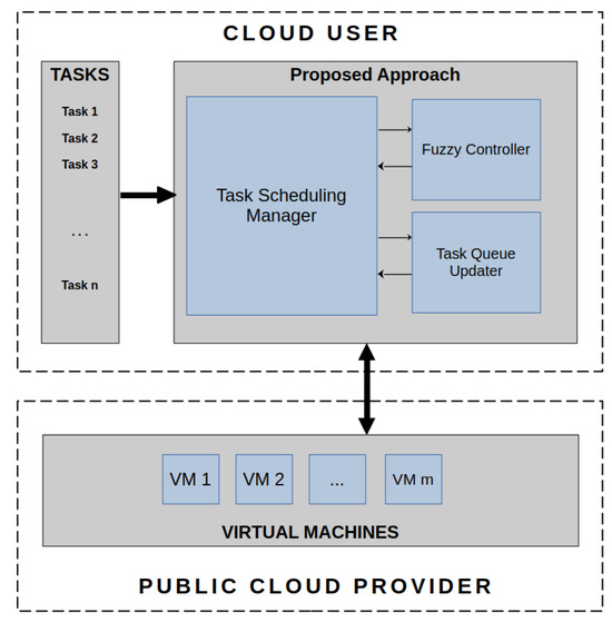
Figure 1.
Schematic diagram of the proposed FPD approach.
The high-level operation of the proposed approach is described in Figure 2 in the form of a flowchart. The proposed approach receives the set of tasks to be processed using public cloud. The first procedure to perform is to obtain the number of VMs that will be needed to execute the tasks, as well as the tasks that each of those VMs will receive. This part is accomplished with the help of the proposed fuzzy controller. The fuzzy controller initializes a VM list and starts checking the compatibility of each task for the VMs in the VM list. A task is assigned to the first VM that satisfies its requirements. After all the tasks have been assigned to their respective VMs, the fuzzy controller forwards the VM–task mapping to the next stage of the proposed approach. This stage sorts the tasks on each VM first according to the order of their deadlines, with earliest deadlines coming first. Then it further sorts the tasks such that high-priority tasks are brought to the head of the task list. Finally, the sorted and mapped task list is sent to be processed on the public cloud.
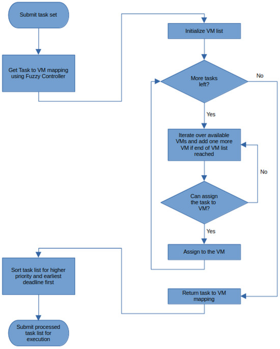
Figure 2.
Flowchart of the proposed approach.
Algorithm 1 describes the operation of the proposed FPD task scheduling approach. In lines 1–3, the task characteristics that are part of each task’s tuple are arranged into separate sets for length, deadline, and priority of tasks. In line 4, the algorithm creates an empty sorted task list that will contain the task scheduling information for the processing of the task set on the public cloud. Then, in line 5, a call is made to the fuzzy controller, with task length and priority inputs passed as arguments. This call returns a mapping from tasks to the number of VMs that will be required. Following this, in lines 6 to 10, the algorithm iterates over the total number of VMs and sorts the tasks assigned to each VM, first by the deadline (earliest first), then by priority (highest priority first). This causes the task queue on each VM to have higher-priority tasks before lower priority-tasks, with a further ordering by deadline (earliest first). The sorted list resulting from each iteration of this loop is added to the final sorted task list (). Finally, in line 11, is submitted to the public cloud for processing.
| Algorithm 1 Proposed FPD Scheme |
Input: Output: void
|
3.1.5. Fuzzy Controller
Algorithm 2 describes the operation of the fuzzy controller that was used in Algorithm 1 to generate the task-to-VM assignment mapping. The fuzzy controller proposed in the present work uses Mamdani fuzzy inference and three fuzzy inputs to make a decision regarding the VM that should execute a given task. The input consists of the crisp-valued inputs for task length and task priority. In line 1, the singleton VM set is created. More VMs are later added to it based on the outputs of the fuzzy controller. The outer for loop iterating over the set of tasks runs from lines 3 to 20. For each task, the approach then iterates over the available VMs in the inner loop and checks the feasibility of assigning the task to each VM. The task is assigned to the first VM that is considered feasible by the fuzzy controller. The fuzzy controller takes as input the fuzzy values for task length, total task length assigned to the current VM, and number of high-priority tasks on the current VM. A fourth input for priority of the current task is used without fuzzification. Its role is to refer to relevant parts of the rule base, since the rule base has two sets of rules: one for each priority type. The applicable rules from the rule base are determined next in line 8. The crisp output is obtained next using strong rules selected using , the threshold of fuzzy controller. If the crisp output value is below 50, then the controller assigns the task to the current VM and continues to the next task. If the output is more than 50, then the task cannot be assigned to the current VM. At this point, if it is found that there are no more VMs in V, the controller adds one more VM to it and checks the feasibility of the task on the next VM. When the outer loop has finished iterating, the VM assignment mapping contains information about the number of VMs that will be needed and the tasks that will be assigned to each VM.
| Algorithm 2 Fuzzy Controller |
Input: Output: VmAssignmentMapping
|
In Mamdani fuzzy reasoning, the fuzzy membership values for crisp inputs are used in the inference rules. The fuzzy input membership functions (MFs) used by the fuzzy controller in the proposed approach are detailed next. The crisp domains of the fuzzy sets used by the proposed fuzzy controller are defined for the target input datasets. In Figure 3a, the fuzzy MF for the task length is given. This MF has four linguistic variables: Small (SM), Medium (ME), Large (LA), and Very Large (VL). The second fuzzy input is for the total load assigned to a VM, and it is defined by the membership function given in Figure 3b. Here, the linguistic variables are Low Load (LO), Medium Load (ME), Heavy Load (HE), and Very Heavy Load (VH). The third fuzzy input is given in Figure 3c and represents the number of high-priority tasks on a VM. It has three variables: Low (LO), Medium (ME), and High (HI) numbers of high priority tasks. The output membership function has two variables: Current VM (CV) and Next VM (NV). The two variables correspond to the decision to map or not map a task to the current VM under consideration. The membership function for output is shown in Figure 3d. In all four membership functions given in Figure 3, the x-axis represents the crisp input or output values and they vary according to the variable being fuzzified or defuzzified. The y-axis represents the fuzzy membership value and it ranges from 0 to 1.
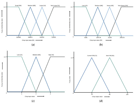
Figure 3.
(a) Fuzzy membership function for task length. (b) Fuzzy membership function for total task length assigned to a given VM. (c) Fuzzy membership function for number of high-priority tasks on a VM. (d) Fuzzy membership function for output regarding task assignment decision.
The fuzzy rule base used in the proposed fuzzy controller is shown in Figure 4. The fuzzy rule base is defined using three fuzzy and one crisp input. It contains a total of 96 rules that were obtained through extensive experimentation on a synthetic dataset explained later. Input 1 is the task length, Input 2 is the total task length assigned to the VM, and Input 3 is the number of high-priority tasks on the VM. The rule base is divided into two parts based on the priority of the task. In the present work, the minimum value among all the fuzzy input values in an applicable rule is used to calculate the firing value of the output. Strong rules were selected using a threshold value (), with all the rules having fuzzy output values equal to or above the chosen . From the strong rules firing values for each fuzzy output set, the minimum firing values were chosen for each set.
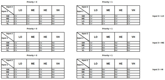
Figure 4.
The fuzzy rule base used in the proposed approach.
The final step in obtaining the crisp output was defuzzification, and it was performed using the Center-of-Gravity method (CoG) using Equation (1).
where is the curve enclosing the region formed by the intersection of output membership functions with the output firing values obtained from strong rules. is the x coordinate of the CoG of the aforementioned enclosed area.
3.1.6. Computational Complexity
As seen previously, the proposed approach is divided into two parts: the main algorithm and the call to the fuzzy controller. The fuzzy controller part is found to have a worst-case time complexity of , since it has two nested loops. The outer loop runs m times, and the inner loop runs n times, corresponding to the number of VMs and number of tasks, respectively. The main part of the algorithm also has two nested loops such that the outer loop runs m times and the inner loops perform sorting operations over a maximum of n tasks. Since the worst-case time complexity of sorting is , the worst-case time complexity of the nested loops in the main algorithm is . This is also the worst-case time complexity of the proposed approach overall. For larger datasets, the time taken by the proposed approach should increase polynomially. However, for very large task sets, the scalability of the proposed approach is limited by any hard limits on the number of VMs that may be obtained from a particular public cloud.
3.2. Experimental Setup
The testing of various scenarios of resource usage optimization in cloud computing is a necessary part of arriving at an informed decision regarding the usefulness of a given scenario. Testing can be performed on a real-world cloud testbed, but that can be cost-prohibitive. There is also a plethora of simulation software available for the simulation of task scheduling schemes without using a real-world test bed. Such software does not require extensive hardware setups and is flexible in terms of the scenarios that it can test [32]. One of the more prominent examples of such software is CloudSim, which is an event-based simulator for the testing of cloud usage scenarios. Tests in the current study were conducted using version 3.0.3 of CloudSim [33]. The details of the system used to run CloudSim are provided in Table 2.
Table 2.
Hardware and software details of the system used in this study.
The present work is aimed at task scheduling on public clouds in general and the AWS public cloud in particular. Thus, the VMs used in the current study have the same configuration as the c8g.large compute optimized EC2 instance provided by AWS. The details of the parameters for the VMs are presented in Table 3. A simplifying assumption was made in terms of keeping the number of instructions executed per second the same as the CPU clock frequency.
Table 3.
Details of parameters of the used VMs.
Two different task sets were used to test the performance of the proposed approach: a randomly generated synthetic task set and the GoCJ task set, which was developed to have characteristics similar to those of the Google Cluster task set [38]. The priority input for the task set had two priority levels: high and low. It was generated such that the probability of occurrence of high-priority tasks was 0.1. Deadline was generated using , where is the stringency value or tightness of the deadline and was set to 1.2 as per previous literature [39].
3.3. Performance Measures
The proposed approach was compared with other task scheduling approaches using a number of performance measures, which are briefly described below:
- Total number of VMs: The total number of VMs used by a given approach to process all the tasks in the task set.
- Degree of Imbalance (DoI): Used to provide a measure of the variation in the relative finishing times of the used VMs, expressed as follows:
- Makespan: The final time to complete all the tasks.
- Total cost: Sum of the total cost incurred by all VMs, expressed as follows:
- Average completion time of various tasks: The average finishing times of a subset of tasks among the complete task set. This metric has is obtained for high- and low-priority subsets of the task set.
- Average waiting time of various tasks: Average waiting time of a subset of tasks computed for-high priority, low-priority, and all tasks. The average waiting time of a single task is expressed as follows:
- Total time under SLA violation: This is the time spent beyond the deadline of high-priority tasks.
- Total SLA violation count: The total number of tasks that miss their SLA deadlines.
- Total high-priority SLA violation count: The total number of high-priority tasks that miss their SLA deadlines.
4. Results
This section presents a comparison of the results of the proposed approach for various threshold levels with results obtained for synthetic and GoCJ datasets. The results are presented in the form of graphs with, the x-axes of all graphs denoting the number of tasks used for a given measurement point and the y-axes are also suitably labeled as the performance measure being displayed by a particular graph. The proposed work is compared against FCFS-EDF, SJF-EDF, and Random-EDF, which are all standard heuristic approaches that have been used as benchmarks for the testing of the performance of task scheduling approaches in the literature.
The graphical results for threshold selection and the two datasets are presented in Figure 5, Figure 6, Figure 7, Figure 8, Figure 9, Figure 10, Figure 11, Figure 12 and Figure 13 in the subsequent subsections. The results in the aforementioned figures are explained in the accompanying text in terms of average percentage improvements. The average percentage improvement for the threshold graphs in Figure 5, Figure 6 and Figure 7 and for the proposed approach at the selected threshold in Figure 8, Figure 9, Figure 10, Figure 11, Figure 12 and Figure 13 are obtained using the expression given below.
where denotes the average percentage improvement of the proposed approach compared to a competing threshold or approach for a given performance measure (j). The total number of measured values is given by p, while the values of the proposed approach and the compared threshold (or approach) for a given j and k are given by and , respectively.
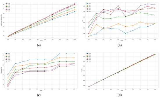
Figure 5.
(a) The total number of VMs used by the proposed approach for different threshold levels. (b) The degree of imbalance of the finish times of the VMs. (c) The makespan achieved at different threshold levels. (d) Total cost incurred.
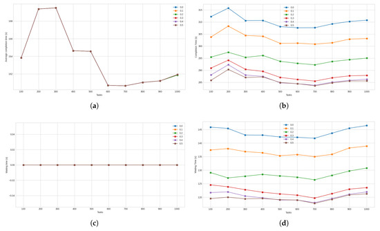
Figure 6.
(a) Average completion time for high-priority tasks. (b) Average completion time for low-priority tasks. (c) Average waiting time for high-priority tasks. (d) Average waiting time for low-priority tasks.
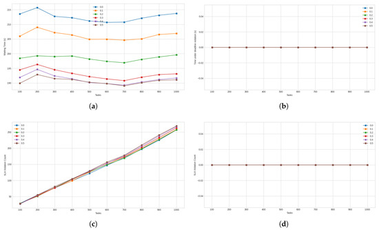
Figure 7.
(a) Average waiting time for all tasks. (b) Total time spent on high-priority tasks beyond their deadlines. (c) Total number of tasks of all priority levels that undergo SLA violation. (d) Total number of high-priority task that undergo SLA violation.
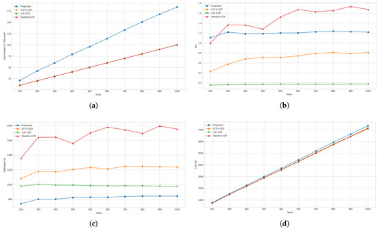
Figure 8.
(a) Total number of VMs required by the proposed and compared approaches. (b) Degree of imbalance between finish times of all the VMs. (c) Makespans achieved by all approaches. (d) Total costs to execute the tasks.
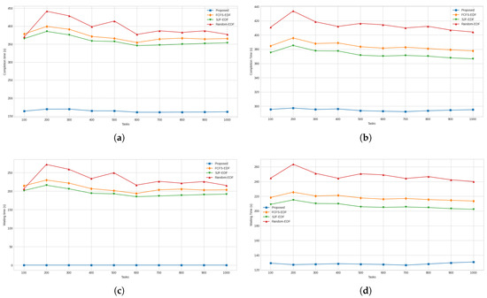
Figure 9.
(a) Average completion times for high-priority tasks. (b) Average completion times for low-priority tasks. (c) Average waiting times for high-priority tasks. (d) Average waiting times for low-priority tasks.
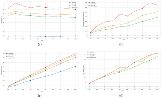
Figure 10.
(a) Average waiting times for all tasks. (b) Total SLA violation times of high-priority tasks. (c) Total number of SLA violations for all tasks. (d) Total number of SLA violations for high-priority tasks.
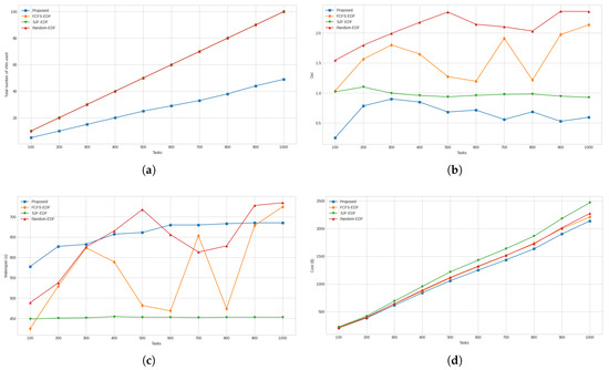
Figure 11.
(a) Total number of VMs required by the proposed and compared approaches. (b) Degree of imbalance between finish times of all the VMs. (c) Makespans achieved by all approaches. (d) Total costs to execute the tasks.
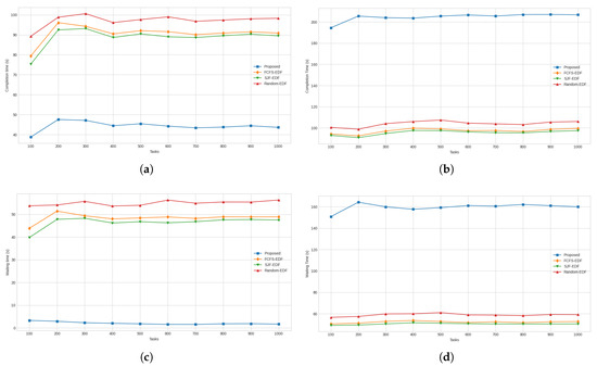
Figure 12.
(a) Average completion times for high-priority tasks. (b) Average completion times for low-priority tasks. (c) Average waiting times for high-priority tasks. (d) Average waiting times for low-priority tasks.
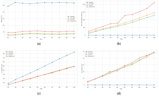
Figure 13.
(a) Average waiting times for all tasks. (b) Total SLA violation times of high-priority tasks. (c) Total number of SLA violations for all tasks. (d) Total number of SLA violations for high-priority tasks.
4.1. Threshold
To arrive at the optimum threshold value to determine strong rules, the authors ran the proposed approach for values threshold values from and using a synthetic workload. At , the fuzzy approach was found to degrade heavily in functionality, whereas the lower threshold values often achieved results close to each other. Plotting results for , along with the lower threshold values, was found to cause the differences between lower threshold values to become less discernible. Thus, only the comparative graphs of results obtained for threshold values between 0.0 and 0.5 are presented in this subsection.
Figure 5a, shows the total number of VMs used at each threshold. Compared to thresholds and , was found to require 13.48% and 8.16% more VMs, respectively, whereas for thresholds , , and , it required 5.66%, 8.33%, and 8.44% fewer VMs, respectively. The degree of imbalance between the finish times of VMs for various threshold levels is shown in Figure 5b. When comparing the performance of against and , it was found to have a 9.69%, and 7.05% higher degree of imbalance, respectively. Compared to , , and , it had a 3.18%, 4.09%, and 3.32% lower degree of imbalance, respectively. Figure 5c shows the graphs for makespan achieved at various threshold levels. It was found that had a 3.89% and 1.83% lower makespan compared to and , respectively, and a 1.49%, 2.94%, and 2.98% higher makespan than , , and , respectively. This can be attributed to the number of VMs used at the aforementioned thresholds, with the use of a higher number VMs contributing to a lower makespan. In Figure 5d, it is found that, in terms of total cost, is superior to all the other thresholds, with improvements ranging from 0.30% for to 1.64% for .
Graphs showing the performance of the proposed approach at various threshold levels and the average completion times for high-priority tasks are presented in Figure 6a. It was determined that there was no difference between any of the considered thresholds for this measure. The results for average completion times for low-priority tasks are shown in Figure 6b. Here, achieved 5.31% and 2.89% lower completion times compared to and , respectively. Compared to , , and , it required 2.04%, 2.72%, and 2.95% more time, respectively, on average, to complete the low-priority tasks. The average waiting time for high-priority tasks was zero for all the compared threshold values, and the graph summarizing this result is presented in Figure 6c. The graph for average waiting time incurred for low-priority tasks is presented in Figure 6d. For this measure, it was found that had a 12.20%, and 6.63% lower waiting time when compared to and , respectively. On the other hand, it incurred a 4.68%, 6.26%, and 6.79% longer waiting time compared to , , and , respectively.
Figure 7a presents the outputs for average waiting time for all tasks. It was found that for , the waiting time was 7.10% and 3.86% shorter than the waiting times for and , respectively. On the other hand, its waiting time was 2.72%, 3.63%, and 3.94% longer than that for , , and , respectively. The next measure to consider is the total time spent beyond on high-priority tasks beyond the deadline, which is presented in Figure 7b. All the threshold levels under consideration managed to complete their high-priority tasks within their respective deadlines, all obtaining a value of zero for this measure. Thus, there was no variation among the different threshold levels. Figure 7c presents the total SLA violations incurred for all tasks. Regarding this measure, it was found that was better than and by 0.37% and 0.03%, respectively and worse than , , and by 1.09%, and 2.61%, and 3.92%, respectively. In Figure 7d, it can be seen that SLA violation count for all the considered threshold values was zero. As a result, there was no variation between the various threshold levels for this measure. The primary objective of the proposed approach is to ensure that no high-priority tasks miss their SLA deadline. The comparative threshold results show that on this metric, all the compared threshold values were successful. Although did not have the shortest makespan, it provided the lowest cost out of all the threshold values. Therefore, was chosen as the threshold for the proposed approach.
4.2. Synthetic Workload
The proposed approach was first compared using a synthetic workload. This workload was generated for 1000 tasks, with the task lengths randomly varying within the range of 15,000 Million Instructions (MI) to 900,000 MI. Random workloads are commonly used in cloud computing research [22]. The task-length range was chosen to be the same as the GoCJ workload [38] for better comparison between the two workloads. In order to reduce the effect of anomalies in a particular task set affecting the results, six sets of workload were generated. For each of the six sets of workload, a separate deadline input set was generated. The priority input also consisted of six different priority sets. The simulation was run for the six sets so obtained, and the final result was obtained by averaging the results of the six simulations.
The total numbers of VMs used by proposed and compared approaches are presented in Figure 8a. Comparing these results, it was found that the proposed approach used 48.59% more VMs than the other three approaches. When considering this result, it needs to be understood that the proposed approach determines the number of VMs that will be needed for a task set of a particular size and characteristics. On the other hand, the other compared approaches assign the number of VMs using a less informed guess based on the number of tasks they will be required to execute, with 10 VMs allocated for every 100 tasks. The DoI of all the approaches is presented in Figure 8b. Comparing the approaches for this measure, it was found that the proposed approach was worse than FCFS-EDF and SJF-DF by 41.71% and 86.16%, respectively. On the other hand, it was better than Random-EDF by 23.45%. In Figure 8c, the graphs for the makespans achieved by various approaches are shown. Comparing the results, it was determined that the proposed approach was better than FCFS-EDF, SJF-EDF, and Random-EDF by 47.26%, 20.49%, and 103.37%, respectively. Figure 8d shows the graphs for the total costs incurred by all the approaches. The proposed approach incurred 3.91%, 3.30%, and 3.30% more total cost to process the task set compared to the FCFS-EDF, SJF-EDF, and Random-EDF approaches, respectively.
With respect to task-specific performance measures, the results for the average completion time of high priority tasks are presented in Figure 9a. When comparing with the other approaches, it was found that the proposed approach provided an average improvement of 127.24%, 119.35%, and 141.99% against FCFS-EDF, SJF-EDF, and Random-EDF, respectively. Figure 9b presents the graphs for the average completion times of low-priority tasks. When considering this metric, it was found that the proposed approach was superior to FCFS-EDF, SJF-EDF, and Random-EDF by 30.47%, 26.75%, and 40.52%, respectively. As shown by the graph for average waiting times for high-priority tasks presented in Figure 9c, it was found that the proposed approach had a zero waiting time and was superior to all the compared approaches. The average waiting times for low-priority approaches are presented in Figure 9d. For this measure, the proposed approach achieved 70.01%, 61.48%, and 93.13% lower waiting times compared to FCFS-EDF, SJF-EDF, and Random-EDF, respectively.
The results for the average waiting time for all tasks are presented in Figure 10a. For this measure, the proposed approach was better than FCFS-EDF, SJF-EDF, and Random-EDF by 51.30%, 45.68%, and 65.94%, respectively. The graphs in Figure 10b summarize the results for total SLA violation time for high-priority tasks. The proposed approach, having achieved zero seconds for this measure, was superior to all the other approaches. Figure 10c shows the graphs for total SLA violations. For this measure, the proposed approach incurred 51.20%, 40.21%, and 58.78% fewer violations compared to FCFS-EDF, SJF-EDF, and Random-EDF, respectively. Figure 10d shows the results for the number of high-priority tasks that underwent SLA violation. For this measure, again, the proposed approach obtained zero violations and was superior compared to the other three approaches.
4.3. GoCJ Workload
The workload used in this study was “GoCJ_Dataset_1000.txt” from the GoCJ workload task set [38]. The GoCJ workload is a popular dataset that recreates the workload features of the Google Cluster workload. Since its publication, it has found use in many works related to task scheduling [9,13]. The task length in this dataset varies from 15,000 MI to 900,000 MI. A deadline file was generated using the workload data and for priority input the six priority sets used for synthetic workload were used. The simulation was run six times using the six combinations of inputs, with the final result being obtained by averaging the results of all six input sets.
The results for total number of VMs used for task scheduling are presented in Figure 11a. The proposed approach was found to require 103.82%, 103.82%, and 103.82% fewer VMs than the FCFS-EDF, SJF-EDF, and Random-EDF approaches, respectively. The graphs for DoI are presented in Figure 11b and show that, again, the proposed approach is superior to the other three approaches. For this measure, the improvements were found to be 161.28%, 69.45%, and 248.32% against the FCFS-EDF, SJF-EDF, and Random-EDF approaches, respectively. Considering the results for makespan presented in Figure 11c, it was found that the proposed approach required 14.17%, 30.97%, and 2.89% more makespan compared to FCFS-EDF, SJF-EDF, and Random-EDF, respectively. As shown by the graphs presented in Figure 11d, it was found that FCFS-EDF, SJF-EDF, and Random-EDF were 4.72% 13.03%, and 4.74% more expensive compared to the proposed approach, respectively.
For the performance measure concerning average completion time for high-priority tasks, as shown in Figure 12a, the three compared approaches required 104.76%, 100.15%, and 119.59% more time than the proposed approach, respectively. However, when considering the average completion time for low-priority tasks, the proposed approach was found to require 52.49%, 53.34%, and 49.19% more time compared to FCFS-EDF, SJF-EDF, and Random-EDF, respectively. The graphs for this measure are presented in Figure 12b. Moving to the results for average waiting times for high-priority tasks, as presented in Figure 12c, the proposed approach had a clear advantage over the compared approaches. Compared to the proposed approach, the FCFS-EDF, SJF-EDF, and Random-EDF approaches took 2399.69%, 2303.57%, and 2734.45% more waiting time, respectively. The next metric under consideration was average the waiting time for low-priority tasks, and for this metric, the proposed approach required 67.28%, 68.37%, and 63.05% more time compared to FCFS-EDF, SJF-EDF, and Random-EDF, respectively. The graphs for this metric are presented in Figure 12d.
The results for the average waiting times for all tasks are presented in Figure 13a. For this metric, it was seen that the proposed approach required 55.38%, 56.45%, and 51.34% more waiting time overall compared to FCFS-EDF, SJF-EDF, and Random-EDF, respectively. The graph for the total SLA violation time for high-priority tasks is presented in Figure 13b. For this measure, the proposed approach achieved a perfect result, with zero SLA violation time for high-priority tasks. Therefore, it is clearly better than the compared approaches. Figure 13c presents the results for the total number of SLA violations. For this measure, the proposed approach faced a 42.01%, 40.70%, and 40.88% higher total number of SLA violations compared to FCFS-EDF, SJF-EDF, and Random-EDF, respectively. However, as evidenced by the next measure, all the SLA violations faced by the proposed approach were for low-priority tasks. Finally, with respect to the total number of SLA violations that occurred for each approach, as shown by the graph in Figure 13d, the proposed approach faced no SLA violations for high-priority tasks and, thus, is better than the compared approaches for this measure.
5. Discussion
Based on the results of the synthetic dataset, it is observed that the proposed FPD approach is superior to FCFS-EDF, SJF-EDF, and Random-EDF with respect to almost all performance measures. For the number of VMs, DoI, and cost, it showed inferior results relative to those of the compared approaches. However, when it is considered that the proposed approach was able to succeed under the main constraints of the problem, viz., high-priority SLA and makespan, the inferior results in non-primary performance measures may be overlooked. Furthermore, it is observed that the rise in cost of the proposed approach is an order of magnitude lower than the increase in the number of VMs utilized compared to the other approaches. Considering the results for the metric of time spent under SLA violation, if it is used to compute a financial penalty, then the differences in the cost of proposed approach compared to the other approaches will be reduced even further, if not entirely inverted.
For the GoCJ dataset, the proposed approach was found to still meet one of the primary constraints of completing high-priority SLA tasks at any cost. The proposed approach provided worse results for some measures, especially those that concern low-priority tasks. However for the requirements of this study, the primary focus is on high-priority tasks. The makespan, although more than that for the compared approaches, was offset by the lower cost achieved compared to the other techniques. The proposed approach also demonstrated the ability to reduce the number of VMs compared to the other approaches and was still able to meet its constraints. The number of VMs being reduced for the second dataset is explained by the long-tailed distribution of task lengths followed by the GoCJ dataset, which means that most of the tasks contained in it were small in length [38]. On the other hand, all task lengths were equally likely in the synthetic dataset. This means that the total task length in the GoCJ dataset was shorter than that for the synthetic dataset. The proposed approach was designed to determine the number of VMs after taking the task length of individual tasks and, by extension, the combined task lengths of all the tasks into account. This resulted in it using a lower number of VMs for the GoCJ dataset compared to the synthetic dataset. The compared heuristic approaches, on the other hand, were not capable of making informed decision about the number of VMs to use, hence they were restricted to using the same number of VMs for the two datasets.
In order to justify that the superiority of the proposed FPD approach compared to FCFS-EDF, SJF-EDF, and Random-EDF, a weighted ranking system was used. For each performance measure, the best performing approach out of the four was given a score of 4, the next to best approach was given a score of 3, and so on, with the approach coming last getting a score of 1. The performance measures concerning high-priority tasks were multiplied by a weight of 2, while all other measures were multiplied by a weight of 1. For each approach, the average of its scores over the 12 performance measures was used to give it a final rank. The final scores of the approaches according to this method for both datasets are summarized in Table 4. In the table, it can be seen that the proposed approach obtains the highest score for both datasets and is, thus, superior to all the compared approaches.
Table 4.
Ranking of compared approaches for synthetic and GoCJ datasets.
The ability of the presented two-phase fuzzy controller-based approach to determine the number of VMs to rent based on the properties of the input task set gives it an advantage compared to the usual task scheduling approaches in the literature that are not able to determine the number of VMs that will be needed. The scalability of public clouds means that this ability in a task scheduling approach is vital to making full use of public clouds. Furthermore, the present study shows that having the ability to use a variable number of VMs, along with the updating of task queues on each VM, allows for the scheduling of tasks such that the SLA constraint of meeting the deadlines of higher-priority tasks is satisfied. The results also demonstrate that the proposed approach is also capable of fulfilling task scheduling requirements at a lower cost compared to prior techniques that do not have the ability to vary the number of VMs.
Despite its many benefits and improvements over existing works, there are some limitations of the current work as well. The first limitation is that the fuzzy controller used in this study has not been tuned for further optimization of the results. Secondly, although the time complexity is polynomially bound, it would be better if it were at least quasi-linear to better compete with heuristic approaches. The third limitation is that the proposed approach is designed for a task range specific to the workloads used.
In the future, fuzzy controllers may be developed for hybrid cloud scenarios with more than two priority levels. Further tuning of membership functions is also a logical next step to undertake after the current study. Developing the ability to handle workloads with different task-length characteristics, compared to being restricted to task sets following only a single task-set characteristic, is another future avenue for improvement of the current work.
Author Contributions
Conceptualization, S.Q., N.A. and P.M.K.; methodology, S.Q.; software, S.Q.; validation, S.Q., N.A. and P.M.K.; formal analysis, S.Q.; investigation, S.Q.; resources, S.Q., N.A. and P.M.K.; data curation, S.Q.; writing—original draft preparation, S.Q.; writing—review and editing, S.Q., N.A. and P.M.K.; visualization, S.Q.; supervision, N.A. and P.M.K.; project administration, N.A. and P.M.K. All authors have read and agreed to the published version of the manuscript.
Funding
This research received no external funding.
Data Availability Statement
The original contributions presented in this study are included in the article. Further inquiries can be directed to the corresponding author.
Conflicts of Interest
The authors declare no conflicts of interest.
Abbreviations
The following abbreviations are used in this manuscript:
| ACO | Ant Colony Optimization |
| AWS | Amazon Web Service |
| DoI | Degree of Imbalance |
| EC2 | Elastic Compute Cloud |
| EDF | Earliest Deadline First |
| FCFS | First Come, First Served |
| IaaS | Infrastructure as a Service |
| PaaS | Platform as a Service |
| PSO | Particle Swarm Optimization |
| QoS | Quality of Service |
| SaaS | Software as a Service |
| SJF | Shortest Job First |
| SLA | Service-Level Agreement |
| USD | United States Dollar |
| VM | Virtual Machine |
References
- Mell, P.; Grance, T. The NIST Definition of Cloud Computing; National Institute of Standards and Technology: Gaithersburg, MD, USA, 2011. [Google Scholar]
- Marinescu, D.C. Cloud Computing: Theory and Practice; Morgan Kaufmann: Burlington, MA, USA, 2017. [Google Scholar]
- Liu, F.; Tong, J.; Mao, J.; Bohn, R.; Messina, J.; Badger, L.; Leaf, D. NIST cloud computing reference architecture. NIST Spec. Publ. 2011, 500, 1–28. [Google Scholar]
- Gartner Forecasts Worldwide Public Cloud End-User Spending to Total $723 Billion in 2025. Available online: https://www.gartner.com/en/newsroom/press-releases/2024-11-19-gartner-forecasts-worldwide-public-cloud-end-user-spending-to-total-723-billion-dollars-in-2025 (accessed on 25 February 2025).
- 2024 State of the Cloud Report|Flexera. Available online: https://info.flexera.com/CM-REPORT-State-of-the-Cloud (accessed on 25 February 2025).
- Yagmahan, B.; Yenisey, M.M. Scheduling practice and recent developments in flow shop and job shop scheduling. In Computational Intelligence in Flow Shop and Job Shop Scheduling; Springer: Berlin, Germany, 2009; pp. 261–300. [Google Scholar]
- Abraham, O.L.; Ngadi, M.A.; Sharif, J.M.; Sidik, M.K.M. Task Scheduling in Cloud Environment—Techniques, Applications, and Tools: A Systematic Literature Review. IEEE Access 2024, 12, 138252–138279. [Google Scholar] [CrossRef]
- Jalali Khalil Abadi, Z.; Mansouri, N. A comprehensive survey on scheduling algorithms using fuzzy systems in distributed environments. Artif. Intell. Rev. 2024, 57, 4. [Google Scholar]
- Kakumani, S.P. An Improved Task Scheduling Algorithm for Segregating User Requests to different Virtual Machines. Master’s Thesis, National College of Ireland, Dublin, Ireland, 2020. [Google Scholar]
- Nabi, S.; Ibrahim, M.; Jimenez, J.M. DRALBA: Dynamic and resource aware load balanced scheduling approach for cloud computing. IEEE Access 2021, 9, 61283–61297. [Google Scholar]
- Hussain, M.; Wei, L.F.; Lakhan, A.; Wali, S.; Ali, S.; Hussain, A. Energy and performance-efficient task scheduling in heterogeneous virtualized cloud computing. Sustain. Comput. Inform. Syst. 2021, 30, 100517. [Google Scholar]
- Yadav, M.; Mishra, A. An enhanced ordinal optimization with lower scheduling overhead based novel approach for task scheduling in cloud computing environment. J. Cloud Comput. 2023, 12, 8. [Google Scholar] [CrossRef]
- Qamar, S.; Ahmad, N.; Khan, P.M. A novel heuristic technique for task scheduling in public clouds. In Proceedings of the 2023 International Conference on Advanced Computing & Communication Technologies (ICACCTech), Banur, India, 23–24 December 2023; IEEE: Piscataway, NJ, USA, 2023; pp. 163–168. [Google Scholar]
- Pirozmand, P.; Hosseinabadi, A.A.R.; Farrokhzad, M.; Sadeghilalimi, M.; Mirkamali, S.; Slowik, A. Multi-objective hybrid genetic algorithm for task scheduling problem in cloud computing. Neural Comput. Appl. 2021, 33, 13075–13088. [Google Scholar] [CrossRef]
- Sahoo, S.; Sahoo, B.; Turuk, A.K. A learning automata-based scheduling for deadline sensitive task in the cloud. IEEE Trans. Serv. Comput. 2019, 14, 1662–1674. [Google Scholar] [CrossRef]
- Tarafdar, A.; Debnath, M.; Khatua, S.; Das, R.K. Energy and makespan aware scheduling of deadline sensitive tasks in the cloud environment. J. Grid Comput. 2021, 19, 1–25. [Google Scholar] [CrossRef]
- He, X.; Shen, J.; Liu, F.; Wang, B.; Zhong, G.; Jiang, J. A two-stage scheduling method for deadline-constrained task in cloud computing. Clust. Comput. 2022, 25, 3265–3281. [Google Scholar] [CrossRef]
- Chandrashekar, C.; Krishnadoss, P.; Kedalu Poornachary, V.; Ananthakrishnan, B.; Rangasamy, K. HWACOA scheduler: Hybrid weighted ant colony optimization algorithm for task scheduling in cloud computing. Appl. Sci. 2023, 13, 3433. [Google Scholar] [CrossRef]
- Beegom, A.A.; Rajasree, M. Integer-pso: A discrete pso algorithm for task scheduling in cloud computing systems. Evol. Intell. 2019, 12, 227–239. [Google Scholar]
- Ben Alla, S.; Ben Alla, H.; Touhafi, A.; Ezzati, A. An efficient energy-aware tasks scheduling with deadline-constrained in cloud computing. Computers 2019, 8, 46. [Google Scholar] [CrossRef]
- Abdel-Basset, M.; Mohamed, R.; Abd Elkhalik, W.; Sharawi, M.; Sallam, K.M. Task scheduling approach in cloud computing environment using hybrid differential evolution. Mathematics 2022, 10, 4049. [Google Scholar] [CrossRef]
- Shojafar, M.; Javanmardi, S.; Abolfazli, S.; Cordeschi, N. FUGE: A joint meta-heuristic approach to cloud job scheduling algorithm using fuzzy theory and a genetic method. Clust. Comput. 2015, 18, 829–844. [Google Scholar]
- Adami, D.; Gabbrielli, A.; Giordano, S.; Pagano, M.; Portaluri, G. A fuzzy logic approach for resources allocation in cloud data center. In Proceedings of the 2015 IEEE Globecom Workshops (GC Wkshps), San Diego, CA, USA, 6–10 December 2015; IEEE: Piscataway, NJ, USA,, 2015; pp. 1–6. [Google Scholar]
- Zavvar, M.; Rezaei, M.; Garavand, S.; Ramezani, F. Fuzzy logic-based algorithm resource scheduling for improving the reliability of cloud computing. Asia-Pac. J. Inf. Technol. Multimed. 2016, 5, 39–48. [Google Scholar]
- Mansouri, N.; Zade, B.M.H.; Javidi, M.M. Hybrid task scheduling strategy for cloud computing by modified particle swarm optimization and fuzzy theory. Comput. Ind. Eng. 2019, 130, 597–633. [Google Scholar]
- Farid, M.; Latip, R.; Hussin, M.; Hamid, N.A.W.A. Scheduling scientific workflow using multi-objective algorithm with fuzzy resource utilization in multi-cloud environment. IEEE Access 2020, 8, 24309–24322. [Google Scholar]
- Wang, J.; Li, X.; Ruiz, R.; Yang, J.; Chu, D. Energy utilization task scheduling for mapreduce in heterogeneous clusters. IEEE Trans. Serv. Comput. 2020, 15, 931–944. [Google Scholar]
- Guo, X. Multi-objective task scheduling optimization in cloud computing based on fuzzy self-defense algorithm. Alex. Eng. J. 2021, 60, 5603–5609. [Google Scholar]
- Understand the Default AWS Limits. Available online: https://docs.bitnami.com/aws/faq/get-started/understand-limits/ (accessed on 18 March 2025).
- Allocation Quotas|Compute Engine Documentation|Google Cloud. Available online: https://cloud.google.com/compute/resource-usage (accessed on 18 March 2025).
- Azure Subscription and Service Limits, Quotas, and Constraints—Azure Resource Manager|Microsoft Learn. Available online: https://learn.microsoft.com/en-us/azure/azure-resource-manager/management/azure-subscription-service-limits (accessed on 18 March 2025).
- Kaleem, M.; Khan, P. Commonly used simulation tools for cloud computing research. In Proceedings of the 2015 2nd International Conference on Computing for Sustainable Global Development (INDIACom), New Delhi, India, 11–13 March 2015; IEEE: Piscataway, NJ, USA, 2015; pp. 1104–1111. [Google Scholar]
- Calheiros, R.N.; Ranjan, R.; Beloglazov, A.; De Rose, C.A.; Buyya, R. CloudSim: A toolkit for modeling and simulation of cloud computing environments and evaluation of resource provisioning algorithms. Softw. Pract. Exp. 2011, 41, 23–50. [Google Scholar]
- Cloud Compute Instances—Amazon EC2 Instance Types—AWS. Available online: https://aws.amazon.com/ec2/instance-types/ (accessed on 9 February 2025).
- ARM Processor—AWS Graviton Processor—AWS. Available online: https://aws.amazon.com/ec2/graviton/ (accessed on 9 February 2025).
- aws-graviton-getting-started/README.md at main · aws/aws-graviton-getting-started · GitHub. Available online: https://github.com/aws/aws-graviton-getting-started/blob/main/README.md (accessed on 9 February 2025).
- EC2 On-Demand Instance Pricing—Amazon Web Services. Available online: https://aws.amazon.com/ec2/pricing/on-demand/ (accessed on 9 February 2025).
- Hussain, A.; Aleem, M. GoCJ: Google cloud jobs dataset for distributed and cloud computing infrastructures. Data 2018, 3, 38. [Google Scholar] [CrossRef]
- Li, X.; Jiang, X.; Garraghan, P.; Wu, Z. Holistic energy and failure aware workload scheduling in Cloud datacenters. Future Gener. Comput. Syst. 2018, 78, 887–900. [Google Scholar]
Disclaimer/Publisher’s Note: The statements, opinions and data contained in all publications are solely those of the individual author(s) and contributor(s) and not of MDPI and/or the editor(s). MDPI and/or the editor(s) disclaim responsibility for any injury to people or property resulting from any ideas, methods, instructions or products referred to in the content. |
© 2025 by the authors. Licensee MDPI, Basel, Switzerland. This article is an open access article distributed under the terms and conditions of the Creative Commons Attribution (CC BY) license (https://creativecommons.org/licenses/by/4.0/).