Data-Driven Diagnostics for Pediatric Appendicitis: Machine Learning to Minimize Misdiagnoses and Unnecessary Surgeries

Abstract

Pediatric appendicitis remains a challenging condition to diagnose accurately due to its varied clinical presentations and the non-specific nature of symptoms, particularly in younger patients. Traditional diagnostic approaches often result in delayed treatments or unnecessary surgical interventions, highlighting the need for more robust diagnostic tools. In this study, we explore the potential of machine learning (ML) algorithms to improve the diagnosis, management, and prediction of appendicitis severity in pediatric patients. Using a dataset of pediatric patients with suspected appendicitis, we developed and compared several ML models, including logistic regression (LR), random forests (RFs), gradient boosting machines (GBMs), and Multilayer Perceptrons (MLPs). These models were trained using clinical, laboratory, and imaging data to predict three key outcomes: diagnosis accuracy, management strategy, and the likelihood of negative appendectomies. Our results demonstrate that the RF model achieved the highest overall performance with an Area Under the Receiver Operating Characteristic curve (AUC-ROC) score of 0.94 for diagnosing appendicitis, 0.92 for determining the appropriate management strategy, and 0.70 for predicting appendicitis severity. Furthermore, by employing advanced feature selection techniques, the models were able to reduce the number of unnecessary surgical interventions by up to 17%, highlighting their potential for clinical application. The findings of this study suggest that ML models can significantly enhance diagnostic accuracy and provide valuable insights for managing pediatric appendicitis, potentially reducing unnecessary surgeries and improving patient outcomes.

1. Introduction

Children under 5 years old often present with non-specific symptoms, making the diagnosis of acute appendicitis challenging. Communication difficulties and limitations in conducting thorough physical examinations further contribute to the high misdiagnosis rate in this age group. Consequently, delayed diagnosis increases the risk of complications such as perforation and abscess formation. Factors like a thin-walled appendix and inadequate omental barrier also contribute to the likelihood of perforation. The list of potential differentials includes conditions like acute gastroenteritis and respiratory or urinary tract infections. Chang et al. [1] conducted a clinical study highlighting the substantial misdiagnosis rate, ranging from 70 to 100% in children aged 3 and younger, with preschool-aged children experiencing rates of 19 to 57% (with perforation observed in 43% to 72% of cases). This rate decreased to 12 to 28% in school-age children and less than 15% in adolescents. Alarmingly, up to 15% of patients underwent multiple emergency department visits before a correct diagnosis of acute appendicitis was established. Common characteristics among misdiagnosed patients included a relatively short duration of symptoms at the initial visit, presentation during late-night hours, fewer physical examination findings, and inadequate investigation. The risk of misdiagnosis escalates with younger age, with young children facing a five-fold higher risk of complicated appendicitis.

In this study, we aim to explore the role of ML algorithms in diagnosing pediatric appendicitis, focusing on their ability to predict the severity, management strategy, and likelihood of negative appendectomies. We employ a range of supervised learning techniques to analyze a dataset collected from pediatric patients presenting with suspected appendicitis. By comparing the performance of models such as logistic regression (LR), random forests (RFs), gradient boosting machines (GBMs), and Multilayer Perceptrons (MLPs), we seek to demonstrate the potential of ML to enhance diagnostic accuracy and provide actionable insights in clinical practice.

This research not only contributes to the growing body of literature on the application of ML in healthcare but also aims to inform future efforts to integrate these models into clinical workflows. Our findings underscore the need for further validation of ML-based tools in larger, more diverse patient populations, as well as the importance of addressing practical and ethical concerns in their implementation.

In particular, the originality and contribution of this work can be denoted as follows:

• The study applies ML models to pediatric appendicitis diagnosis, which is an area with limited existing research focused on this specific patient group;
• We introduce a novel feature selection approach that combines clinical, laboratory, and imaging variables to improve diagnostic accuracy and predict appendicitis severity;
• The research evaluates multiple ML algorithms, offering a comparative analysis of their performance in clinical settings;
• Our work addresses the challenge of negative appendectomies by incorporating models designed to predict unnecessary surgeries, providing insights that could reduce surgical interventions and improve patient outcomes;
• This study lays the groundwork for the future integration of ML models into clinical workflows, emphasizing practical considerations such as interpretability and clinical relevance.

The remainder of this paper is structured as follows. Section 2 reviews the related work, while Section 3 discusses the theoretical background related to pediatric appendicitis and the deployed ML models. Section 4 presents a detailed overview of the dataset and the methodology used for feature selection and model training. Furthermore, it discusses the experimental setup, including the evaluation metrics and cross-validation techniques. Finally, Section 5 concludes the paper and offers suggestions for future research directions.

2. Related Work

2.1. AI in Pediatric Healthcare

Lupu et al. [2] examine the evolution of diagnostic approaches for Helicobacter pylori infection in pediatric patients, comparing traditional methods, such as urea breath tests and stool antigen tests, with newer molecular techniques. Their findings highlight the strengths and limitations of these diagnostic strategies, emphasizing the importance of accuracy and non-invasiveness in pediatric settings. While their work does not directly address appendicitis, it contributes to the broader discussion on optimizing pediatric diagnostics through a balance of traditional and modern methodologies.

Brind’Amour [3] provides an exploratory overview of artificial intelligence applications in pediatrics, focusing on emerging AI-driven tools for diagnosis, treatment planning, and predictive modeling. The study highlights AI’s potential to improve efficiency and reduce diagnostic errors in clinical settings, particularly in areas requiring rapid and precise decision-making. However, the author also raises concerns regarding data bias, ethical considerations, and the integration of AI models into routine medical practice, making this work a crucial reference when considering the practical implementation of AI in pediatric diagnostics.

Schaefer et al. [4] provide a comprehensive narrative review on AI applications in pediatrics, analyzing its clinical promises and potential pitfalls. Their study differentiates between AI models designed for decision support, imaging analysis, and patient risk stratification, highlighting cases where machine learning outperforms traditional diagnostic criteria. Importantly, they emphasize the gap between theoretical AI advancements and their real-world clinical deployment, pointing to regulatory challenges and lack of generalizability as major obstacles.

Gómez et al. [5] take a more specialized approach, focusing on AI-driven advancements in pediatric healthcare while critically assessing their current clinical value and integration challenges. Their study highlights specific deep learning and natural language processing (NLP) techniques used to assist pediatricians, evaluating their impact on diagnostic speed and accuracy. They argue that, while AI shows significant promise, current datasets remain too fragmented to ensure fully reliable clinical applications.

2.2. Predicting Pediatric Appendicitis Outcomes

Various studies have aimed to improve pediatric appendicitis diagnosis, management guidance, and severity assessment. One notable study by Marcinkevics et al. [6] combined multiple ML algorithms to enhance diagnostic accuracy. Using ensemble learning methods like boosting and bagging, the study compared random forest (RF), gradient boosting machine (GBM), and logistic regression (LR) models. The RF model achieved AUC-ROC scores of 0.94 for diagnosis, 0.92 for management, and 0.70 for severity, showing strong predictive performance. Cross-validation and bootstrap resampling further supported model robustness. However, limitations included data imbalance and the need for external validation.

Another study by Marcinkevics et al. [7] developed interpretable ML models using ultrasound images for predicting pediatric appendicitis outcomes, enhancing clinical decision-making through model transparency. Similarly, Mijwil et al. [8] explored ML models for predicting appendicitis severity, achieving an accuracy of 83.75% with the RF model. The study, although comprehensive, focused on a limited age group (10–30 years), impacting its generalizability to younger pediatric populations.

Pati et al. [9] created a Clinical Decision Support System (CDSS) for early diagnosis by employing an ensemble approach. They compared classifiers like LR, Naïve Bayes, K-nearest neighbor, Support Vector Machine, Decision Tree, RF, Multilayer Perceptron, and Adaboost. Feature selection and optimization were performed using Correlation Feature Selection (CFS) and the Elephant Search Algorithm (ESA). RF, DT, and Adaboost achieved diagnostic accuracies above 91%. Despite the model’s high predictive performance, its reliance on single-center data and lack of external validation are notable limitations.

Together, these studies highlight distinct ML applications for diagnosing pediatric appendicitis. Marcinkevics et al.’s approach provides a robust but computationally intensive solution, while Pati et al. offer a more clinically practical model with strong diagnostic potential, though its reproducibility is less clear.

2.3. Predicting and Reducing Negative Appendectomies

ML has also been applied to enhance appendicitis diagnosis to reduce unnecessary surgeries. Males et al. [10] developed an ML model to minimize negative appendectomies, achieving high sensitivity (0.997) and specificity (0.17), and preventing 17% of unnecessary surgeries. SHAP values were used to assess feature importance. The model’s robustness is validated through nested cross-validation, though it faces limitations such as data imbalance and the need for external validation.

Shahmoradi et al. [11] created a CDSS that compares Multilayer Perceptron and Support Vector Machine models, achieving high specificity (95.0%) and accuracy (96.2%). Despite its clinical relevance, the model’s reliance on single-center data and limited feature selection criteria affect its reproducibility.

Both studies contribute to reducing negative appendectomies through ML. Males et al. provide a robust model emphasizing methodological rigor, while Shahmoradi et al. offer a simpler system designed for clinical integration, highlighting different approaches to optimizing diagnostic precision.

2.4. Predictive Clinical Scoring Systems

Several recent studies focus on clinical scoring systems to differentiate between complicated and uncomplicated appendicitis, aiming to reduce unnecessary surgical interventions. Pogorelić et al. [12] evaluated the Appendicitis Inflammatory Response (AIR) score, finding high sensitivity (89.5%) and specificity (71.9%) for distinguishing perforated from non-perforated appendicitis. However, limitations include data imbalance and lack of external validation.

Van Amstel et al. [13] performed a multicenter evaluation of 12 clinical prediction rules (CPRs) for pediatric appendicitis. The Gorter CPR, validated externally, achieved a sensitivity of 86% and specificity of 91%. The study’s strengths include its rigorous methodology and use of objective variables to improve reproducibility.

Both studies provide valuable insights into scoring systems for pediatric appendicitis, with Pogorelić et al. emphasizing sensitivity and Van Amstel et al. offering a broader multicenter perspective, showcasing the utility of scoring systems in guiding clinical decision-making.

A study by Yazici [14] investigated the predictive performance of six different ML algorithms in distinguishing between simple and complicated acute appendicitis. The authors analyzed data from 1132 patients who underwent emergency appendectomy between 2012 and 2022. They identified significant features such as age, C-reactive protein levels, and periappendicular liquid collection. Among the algorithms tested, k-nearest neighbors and logistic regression achieved the highest accuracy of 96% in the validation group. The study concludes that, using a minimal set of input features, the severity of acute appendicitis can be predicted with high accuracy, offering a practical tool for clinical decision-making.

A comprehensive overview of artificial intelligence (AI) applications in diagnosing acute appendicitis, especially in pediatric cases, is provided by Lam et al. [15]. The authors assess various AI and ML models, analyzing their effectiveness and diagnostic accuracy compared with traditional diagnostic methods. Key findings suggest that AI models, particularly those utilizing image-based diagnostics and clinical feature analysis, can significantly enhance diagnostic precision. However, the review identifies challenges in implementing these models clinically, such as a lack of interpretability, concerns with data quality, and issues with model generalizability across different populations. The study emphasizes the potential of AI to aid in timely and accurate diagnosis, while also highlighting areas that require further development for clinical adoption.

A method for developing interpretable medical risk scores tailored for pediatric appendicitis is presented by Roig Aparicio et al. [16]. The study applies ML techniques to create risk scores that are both clinically interpretable and actionable, helping healthcare providers assess the likelihood of appendicitis and make informed decisions. Using real-world clinical data, the authors demonstrate that their risk scores can effectively guide clinical decisions with a balance of transparency and predictive accuracy. The work underscores the importance of model interpretability in clinical settings, aiming to build trust and utility among healthcare professionals. By focusing on interpretability and real-time clinical application, this approach offers a promising tool for enhancing pediatric appendicitis management.

2.5. Comparison with This Work

This work and the mentioned studies share a focus on using ML and clinical scoring systems to improve the diagnosis of pediatric appendicitis, but differ in methodology and dataset size.

Marcinkevics et al. combine multiple ML algorithms but are limited by a single-center dataset and the need for external validation. This work, with its larger, multicenter dataset, offers more generalizability. Similarly, Pati et al. developed a Clinical Decision Support System (CDSS), but their reliance on a smaller, single-center dataset limits its applicability compared with the broader approach taken in this work. Males et al. focus on reducing negative appendectomies using a highly sensitive ML model. While both studies aim to improve diagnostic accuracy, Males et al. prioritize sensitivity, whereas this work provides a more comprehensive comparison of scoring systems, broadening its clinical impact. Shahmoradi et al. also developed a CDSS but use a small dataset and single-center data, limiting reproducibility. This work surpasses these limitations by leveraging a multicenter dataset, offering more robust results. Pogorelić et al. focus on the Appendicitis Inflammatory Response (AIR) score, showing high sensitivity and specificity, but are limited by single-center data. This work incorporates multiple scoring systems and a broader dataset, offering a more comprehensive diagnostic analysis. Van Amstel et al. evaluate predictive scoring systems in a multicenter setting, similar to this work, but this study’s rigorous comparison of scoring systems provides deeper insights into their performance across various clinical populations.

While each study contributes to improving pediatric appendicitis diagnosis, this work stands out for its multicenter design, broad applicability, and detailed evaluation of multiple scoring systems, offering stronger validation than the other studies.

3. Background

3.1. ML Models

In this study, four different models were employed to predict the diagnosis and severity of pediatric appendicitis: LR, RF, XGBoost, and MLP. Each model was selected for its capacity to handle classification tasks and its potential to enhance diagnostic accuracy in a clinical setting.

LR is a well-established statistical model used for binary classification. It predicts the probability that an observation belongs to one of two classes by applying the logistic function. The model is mathematically represented as:

$$P(Y=1|X)={\displaystyle \frac{1}{1+e^{-({\beta }_0+{\beta }_1{X}_1+\cdots +{\beta }_n{X}_n)}}}$$

where $P(Y=1|X)$ denotes the probability of the outcome being 1 given the predictors X, and the $\beta$ coefficients are estimated from the data. The simplicity and interpretability of LR make it a powerful tool in clinical applications, where understanding the influence of each predictor is important. However, one key limitation of LR is that it assumes a linear relationship between the predictors and the log-odds of the outcome, which may not hold in more complex datasets.

A DT is a non-parametric model that uses a tree-like structure to make decisions based on the input features. The tree recursively splits the data at each node based on a feature that maximizes the purity of the resulting subgroups, using metrics such as Gini impurity or entropy. For example, the Gini impurity is calculated as:

$$G=1-\sum _{i=1}^C{p}_i^2$$

where $p_i$ represents the proportion of class i in a given node. DTs are easy to interpret, as the model’s structure provides a clear path from features to the predicted outcome. Their strength lies in their simplicity and ability to capture non-linear relationships. However, DTs are prone to overfitting, especially when the tree grows deep, capturing noise in the training data.

RF is an ensemble learning technique that builds upon the DT model by constructing multiple trees, each trained on a random subset of the data and features. The final prediction is made by aggregating the predictions from all trees, typically using a majority vote for classification tasks. The mathematical framework behind RF is based on the principle of bagging, which reduces variance by averaging multiple weak learners. The model’s ability to handle high-dimensional datasets and its robustness to overfitting make it particularly useful for complex problems. However, RF models can be computationally expensive, and their interpretability decreases as the number of trees increases, compared with a single DT.

XGBoost, or eXtreme Gradient Boosting, is another ensemble method that improves upon traditional boosting techniques by training sequential DTs to correct the errors of previous trees. The objective function that XGBoost optimizes includes a regularization term to control the complexity of the model, minimizing overfitting. Mathematically, the objective function is:

$$L\left(\theta \right)=\sum _{i=1}^{n}l(y_i,{\widehat{y}}_i)+\sum _{k=1}^K\mathrm{\Omega }\left(f_k\right)$$

where $l(y_i,{\widehat{y}}_i)$ represents the loss function (e.g., log loss for classification), and $\mathrm{\Omega }\left(f_k\right)$ is the regularization term. XGBoost is known for its high performance, particularly in structured datasets, due to its optimization of both speed and accuracy. Its main drawback lies in the complexity of tuning its hyperparameters, such as the learning rate, maximum tree depth, and the number of boosting rounds.

A MLP is a type of feedforward neural network used for classification tasks. A MLP consists of an input layer, one or more hidden layers, and an output layer, where each neuron in one layer is connected to neurons in the next layer. Each neuron’s output is computed as a weighted sum of its inputs passed through an activation function, such as the logistic sigmoid function:

$$\widehat{y}=\sigma (WX+b), \sigma \left(x\right)={\displaystyle \frac{1}{1+e^{-x}}}$$

where W represents the weights, X represents the input, and b is the bias term. The model learns by adjusting these weights using a process called backpropagation, which minimizes the difference between the predicted output and the actual target through gradient descent. MLPs are highly flexible and capable of modeling complex, non-linear relationships in data. However, they are often regarded as “black-box” models due to their lack of interpretability. Additionally, MLPs require significant amounts of data and computational resources, and they are prone to overfitting if not properly regularized.

Each of these models brings distinct advantages and limitations to the task of predicting appendicitis outcomes. LR provides simplicity and interpretability but struggles with non-linear relationships. DTs offer clear interpretability but can easily overfit. RF captures complex interactions between variables and reduces overfitting, though it sacrifices some interpretability. XGBoost delivers high predictive accuracy and robustness but requires careful hyperparameter tuning. MLPs excel at handling non-linear patterns, but their black-box nature and high resource demands can be limited in clinical settings.

3.2. Data Imputation

In many real-world datasets, missing data is a persistent challenge that can compromise the accuracy and reliability of subsequent analyses. This problem occurs when certain values in the dataset are either unobserved or lost due to various reasons such as sensor failures, incomplete surveys, or system errors. Missing data, particularly in heterogeneous datasets containing both continuous and categorical variables, poses a significant problem, as it can lead to biased results or reduce the overall dataset size if handled improperly.

One common approach to mitigate this issue is through data imputation, a process by which missing values are estimated and filled in to maintain the integrity of the dataset.

Given a dataset $X=\{x_1,x_2,\cdots ,x_n\}$, where each $x_i$ is a data point that may include both continuous and categorical features, the Gower distance is a metric that enables the handling of mixed data types. Let each data point, $x_i$, consist of p features, i.e.,

$$x_i=\{x_{i1},x_{i2},\cdots ,x_{ip}\}.$$

For two data points, $x_i$ and $x_j$, the Gower distance, $d_G(x_i,x_j)$, is computed as the weighted sum of individual feature contributions:

$$d_G(x_i,x_j)={\displaystyle \frac{{\sum }_{k=1}^p{w}_k{d}_k(x_{ik},x_{jk})}{{\sum }_{k=1}^p{w}_k}},$$

where:

-

$d_k(x_{ik},x_{jk})$ is the normalized distance between the k-th features of $x_i$ and $x_j$.

-

$w_k$ is a weight assigned to the k-th feature, which is typically 1 if both $x_{ik}$ and $x_{jk}$ are non-missing, and 0 otherwise.

For continuous variables, the distance between two features is the normalized absolute difference:

$$d_k(x_{ik},x_{jk})={\displaystyle \frac{|x_{ik}-x_{jk}|}{max\left(x_k\right)-min\left(x_k\right)}},$$

where $max\left(x_k\right)$ and $min\left(x_k\right)$ denote the maximum and minimum values of the k-th feature across all data points.

For categorical variables, the distance is binary:

$$d_k(x_{ik},x_{jk})=\left\{\begin{array}{cc}0,\hfill & \mathrm{if} x_{ik}=x_{jk},\hfill \\ 1,\hfill & \mathrm{if} x_{ik}\ne x_{jk}.\hfill \end{array}\right.$$

Once the Gower distance is computed between data points, the k-NN algorithm selects the k-nearest neighbors of a data point $x_i$ (those with the smallest Gower distance values) and imputes the missing values by using information from these neighbors. For example, missing values in continuous features may be imputed by the average of the corresponding feature values from the nearest neighbors, while missing categorical values may be imputed using the mode of the neighbors.

In summary, the k-NN imputation process for a missing value in $x_i$ can be expressed as:

$${\widehat{x}}_i={\displaystyle \frac{1}{k}}\sum _{j\in {\mathcal{N}}_k\left(x_i\right)}{x}_j,$$

where ${\mathcal{N}}_k\left(x_i\right)$ represents the set of the k-nearest neighbors of $x_i$ based on the Gower distance.

This combination of k-NN with Gower distance addresses imputation challenges by leveraging both the proximity of data points in a mixed-type feature space and the ability to handle missing values persistently.

4. Experiments

4.1. Dataset Information

In this section, we present a detailed overview of the dataset used to develop ML models for diagnosing pediatric appendicitis. The dataset is derived from a retrospective study conducted at the Children’s Hospital St. Hedwig, with ethical approval from the University of Regensburg’s Ethics Committee [17]. It encompasses 782 observations across 58 variables, covering patient demographics (age, sex, height, weight, BMI), clinical scoring systems (Alvarado Score and Pediatric Appendicitis Score), physical examination findings, laboratory test results, and detailed ultrasound observations. Key target variables of the dataset include:

1.

The patient’s diagnosis, histologically confirmed for operated patients. Conservatively managed patients were classified as having appendicitis if their AS or PAS was ≥4, and the appendix diameter was ≥6 mm.

2.

The management approach, determined by a senior pediatric surgeon, was categorized as either operative (appendectomy: laparoscopic, open, or conversion) or conservative (without antibiotics). Patients undergoing secondary surgery after initial conservative management were considered operatively managed.

3.

The severity of appendicitis, classified as uncomplicated (subacute, fibrosis) and complicated (phlegmonous, gangrenous, perforated, abscessed).

Upon initial exploration, we identified that 30.9% of the data were missing. Notably, variables related to ultrasound findings had at least 40% missing values, a common issue due to operator dependency and variability in emergency settings. Similarly, several urine laboratory tests exhibited high missing rates, likely due to their secondary importance in urgent care scenarios. To address these challenges, variables with over 40% missing data were excluded. As a result, our analysis was focused on a refined dataset comprising 782 observations and 39 variables. After this filtering process, all 782 observations were retained, while only variables with more than 40% missing values were excluded. As a result, the dataset used for modeling included 39 variables instead of the original 58. The remaining gaps (5.5%) were handled using multiple imputation with predictive mean matching (PMM) (m = 5, maxit = 50). While PMM improved data completeness, significant missingness persisted in “RBC in Urine”, “Ketones in Urine”, and “WBC in Urine” (206, 200, and 199 instances, respectively), indicating limitations in capturing predictive relationships.

To enhance imputation reliability, we increased imputations to m = 10, although substantial missing counts remained, prompting us to test other methods. We evaluated linear regression (PMM) and logistic regression (logreg) imputation methods; however, adjustments to the m parameter and model specifications did not fully resolve these gaps. Transitioning to k-nearest neighbors (k-NNs) imputation with Gower distance offered greater flexibility and effectively addressed all remaining missing values in mixed data types.

After preprocessing, statistical examination of the cleaned dataset revealed significant variability in patient characteristics. Key findings include:

• Morphological characteristics: the cohort had a mean age of 11.35 years, an average height of 148.07 cm, and an average weight of 43.18 kg, with notable diversity in body mass. The average BMI was 18.89 kg/m², ranging from underweight to obesity.
• Clinical scores: the average AS was 5.96 and the PAS was 5.27, suggesting moderate appendicitis risk. Scores in this range typically indicate that further diagnostic studies may be necessary, as scores between 5 and 8 are inconclusive, while scores of 1 to 4 are usually negative, and scores of 9 to 10 are diagnostic of appendicitis.
• Physical examination and laboratory tests: average body temperature was 37.41 °C, with some unusually low readings affecting the distribution. The mean WBC count was 12.70 × 10⁹/L and the mean neutrophil percentage was 71.82%, reflecting typical inflammatory responses. CRP (a substance produced by the liver in response to inflammation; elevated levels of CRP indicate an ongoing inflammatory response, which is common in appendicitis) levels had a high right skew with a mean of 31.58 mg/L, indicating a mix of low and high values, consistent with inflammatory conditions.

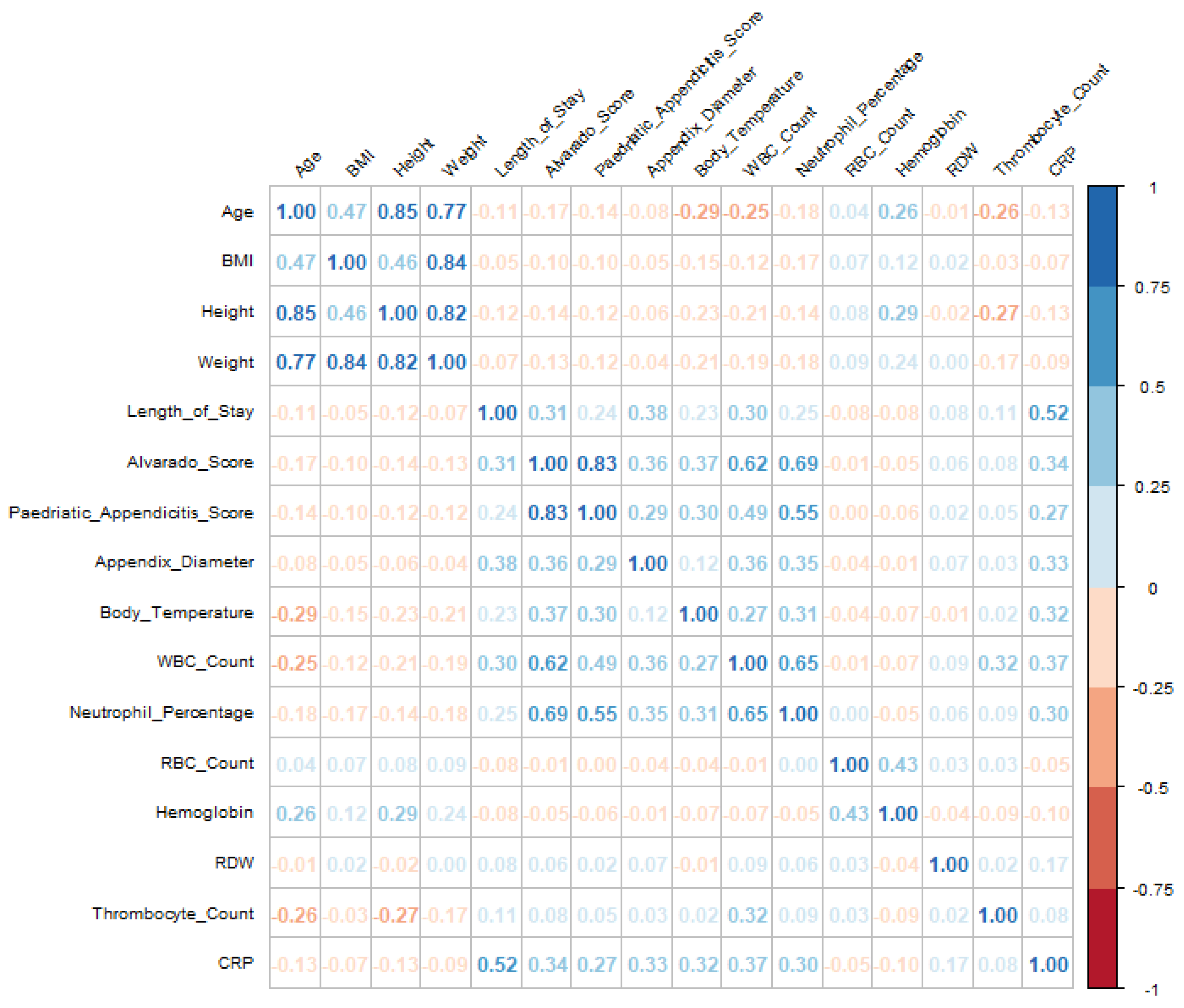
Visualizations, including boxplots and correlation matrices, provided valuable insights into the relationships among key variables, as shown in Figure 1. Before imputation, high missingness limited our ability to analyze relationships among clinical scores, growth metrics, and inflammation markers. However, after preprocessing, the correlation matrix revealed clearer patterns, particularly among growth metrics and age, and between inflammation markers and clinical scores, supporting analyses related to hospital stays and patient outcomes. Notably, correlations between unrelated variables remained low (≤0.40), indicating that imputation preserved authentic variable relationships without inflating associations.

For instance, CRP initially showed a moderate positive correlation with length of stay (0.42), suggesting that higher CRP levels may be associated with longer hospitalizations. Similarly, body temperature demonstrated moderate correlations with both CRP (0.26) and neutrophil percentage (0.28), potentially indicating a link with inflammation. Post-imputation, these relationships were strengthened: the correlation between CRP and length of stay increased to 0.52, while body temperature’s correlations with CRP and neutrophil percentage rose to 0.32 and 0.31, respectively. This enhancement highlights the effectiveness of imputation in improving data reliability, thereby revealing clearer associations among these variables.

4.2. Exploratory Data Analysis

In the exploratory data analysis (EDA) phase, we thoroughly investigated the distributions and interrelationships of key target variables, as depicted by Figure 2. Data were meticulously prepared and visualized using ggplot2 for data visualization, along with dplyr and tidyr for data manipulation, ensuring that actionable insights could be extracted. The analysis revealed that appendicitis was the predominant diagnosis, with 59.5% of patients confirmed to have the condition. Moreover, 61.8% of these cases were managed conservatively, reflecting a significant preference for non-surgical interventions. Severity analysis highlighted that 84.8% of appendicitis cases were classified as uncomplicated, underscoring the effectiveness of conservative management in these scenarios.

Patients diagnosed with appendicitis exhibited significantly higher clinical scores (median AS = 7, PAS = 6) compared with those without the condition (median AS = 5, PAS = 4), demonstrating the effectiveness of these diagnostic tools. Additionally, infection indicators such as WBC count (White Blood Cell, a standard measure in blood tests to check for infections or inflammation) and CRP levels were elevated in appendicitis cases (median WBC count = $14.3\times {10}^9$/L, CRP = 16.0 mg/L), indicating a strong inflammatory response. Further analysis of management strategies revealed that primary surgical management was associated with the highest clinical scores (median AS = 8, PAS = 7) and inflammatory indicators. Patients undergoing surgery also exhibited a higher prevalence of symptoms, such as lower right abdominal pain and nausea, compared with those managed conservatively. This suggests that more severe cases were appropriately triaged to surgical intervention, ensuring targeted and effective care. Finally, severity analysis showed that complicated appendicitis cases had higher median values for clinical scores (median AS = 8, PAS = 6), further validating the diagnostic scoring systems employed.

In summary, the EDA provided critical insights into the dataset, reinforcing the diagnostic utility of clinical scoring systems and highlighting key factors that influence management strategies, which will inform subsequent phases of this study.

4.3. Variable Selection

In this section, we employ several advanced techniques for feature selection and model interpretability, including Recursive Feature Elimination (RFE), Local Interpretable Model-agnostic Explanations (LIME), Shapley Additive Explanations (SHAPs), and Global Feature Explainability models such as RF and GBM. These methods collectively offer a comprehensive view of feature relevance, enhancing both model performance and interpretability.

4.4. Recursive Feature Elimination

RFE is a robust feature selection technique that iteratively fits a model and eliminates the least important features based on model coefficients or importance scores until the optimal subset of features is identified. This process enhances model accuracy and interpretability by reducing the feature space and mitigating the risk of overfitting. The RFE process involves two key steps:

1.

Filtering out incomplete cases: ensuring that only complete data are used for model training.

2.

Defining a cross-validation strategy: a 10-fold cross-validation approach is implemented to balance bias and variance using the refined dataset, which includes 792 observations and 39 variables after handling missing data and feature selection.

In the 10-fold cross-validation strategy, the dataset is randomly partitioned into 10 equal subsets. The model is trained using 9 of these folds (the training set), and the model’s performance is evaluated on the remaining 1 subset (the validation set). This process is repeated 10 times, with each fold serving as the validation set once, ensuring more reliable performance estimates.

The performance of the RFE process is evaluated using two metrics: accuracy and Cohen’s Kappa.

• Diagnosis model: the model’s performance improved with the number of features, reaching optimal results with 19 features. It achieved an accuracy of 96.93% and a Kappa value of 0.9363. The most influential features include appendix diameter, appendix on US, length of stay, Diagnosis Presumptive, and peritonitis.
• Management model: the optimal performance was achieved with 31 features, resulting in an accuracy of 91.95% and a Kappa value of 0.8340. Key features for distinguishing between management strategies include length of stay, appendix diameter, peritonitis, CRP, and neutrophil percentage.
• Severity model: the model performed best with 11 features, attaining an accuracy of 93.60% and a Kappa value of 0.7416. The most critical features are length of stay, CRP, and WBC count, with neutrophil percentage and appendix diameter also playing significant roles.

Following feature selection, we used 19 features for the Diagnosis model, 31 features for the Management model, and 11 features for the Severity model. These selections were made based on Recursive Feature Elimination (RFE) to optimize predictive performance.

In summary, a larger number of features generally enhanced model accuracy and Kappa value for Diagnosis and Management, reflecting the complexity of these tasks. Conversely, the Severity model could be accurately predicted with fewer features, highlighting its more focused nature.

4.5. Local Feature Explainability

Local feature explainability methods provide insights into individual predictions by focusing on specific instances rather than the overall model. This subsection explores two prominent techniques: the Local Interpretable Model-agnostic Explanations (LIME) and Shapley Additive Explanations (SHAPs).

Datasets optimized through RFE were used to train RF models, ensuring explanations were based on the most relevant features.

The optimal number of trees for each target variable was determined by evaluating out-of-bag (OOB) error rates. Here are the findings:

• Diagnosis model: with 450 trees, the model achieved an impressive OOB error rate of 3.45%, indicating high accuracy in distinguishing between appendicitis and non-appendicitis cases.
• Management model: using 750 trees, this model had an OOB error rate of 7.93%. While effective at classifying common management strategies, it struggled with less frequent categories such as secondary surgical management, leading to higher error rates.
• Severity model: employing 650 trees, this model attained a 6.27% OOB error rate, showing strong performance in identifying uncomplicated cases but facing challenges with complex cases.

LIME and SHAP were integrated with RF models using a custom model wrapper that supports prediction and model type identification, facilitating interpretable explanations:

• LIME: provides local explanations by perturbing the input data and fitting a simple, interpretable model to these variations. This approach is useful for understanding individual predictions, such as those for specific patient cases.
• SHAP: offers a theoretically grounded method for evaluating feature importance through Shapley values. It attributes contributions by considering all possible feature combinations, providing both local and global explanations.

While LIME and SHAP enhance interpretability, interpreting their results can be challenging, especially when explanations deviate from clinical expectations. Despite high performance metrics, individual case explanations might not always align with broader patterns, highlighting the need for generalizability and caution against data artifacts.

4.6. Global Feature Explainability

To complement insights from RFE, LIME, and SHAP, we performed a global feature importance analysis using RF and GBM, as per Figure 3, Figure 4, Figure 5, Figure 6, Figure 7 and Figure 8. These techniques offer a comprehensive view of which features most significantly impact model performance across the entire dataset.

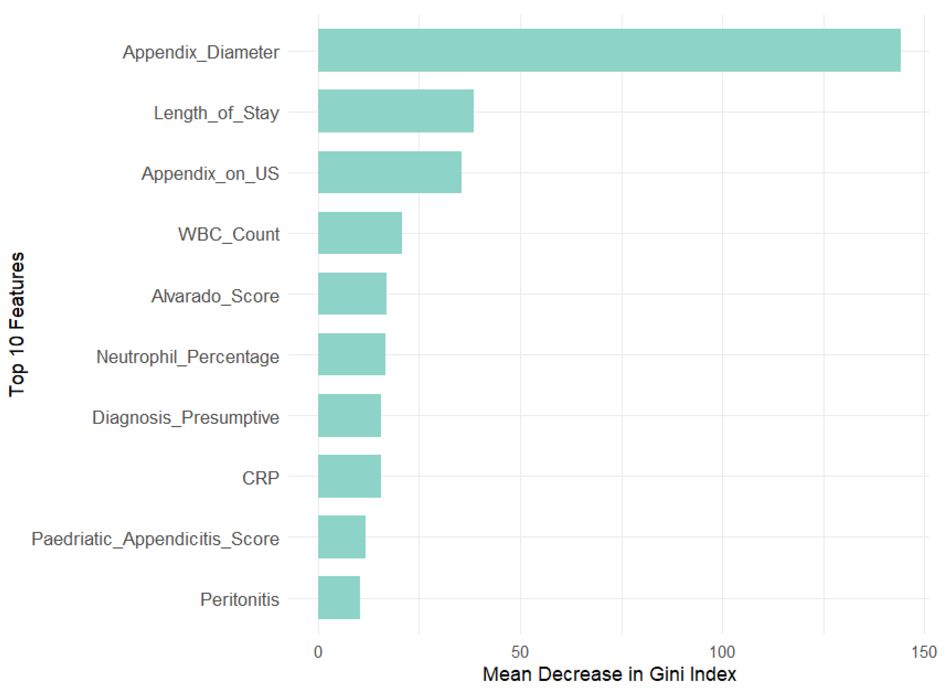
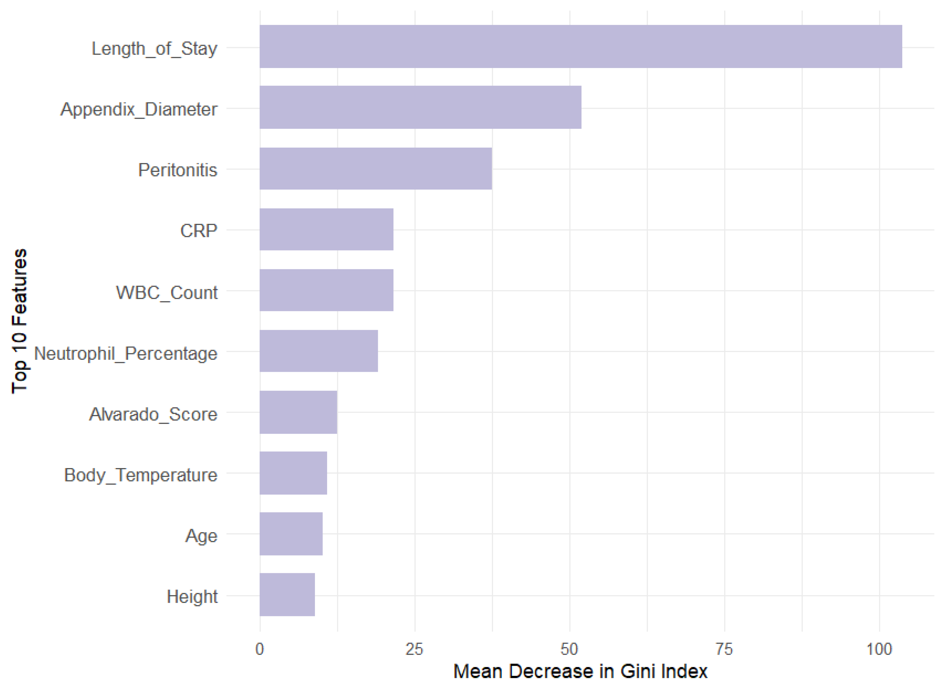
• RF evaluates feature importance using the Mean Decrease in Gini (MDG), which quantifies how much a feature reduces uncertainty or impurity in the model’s predictions.
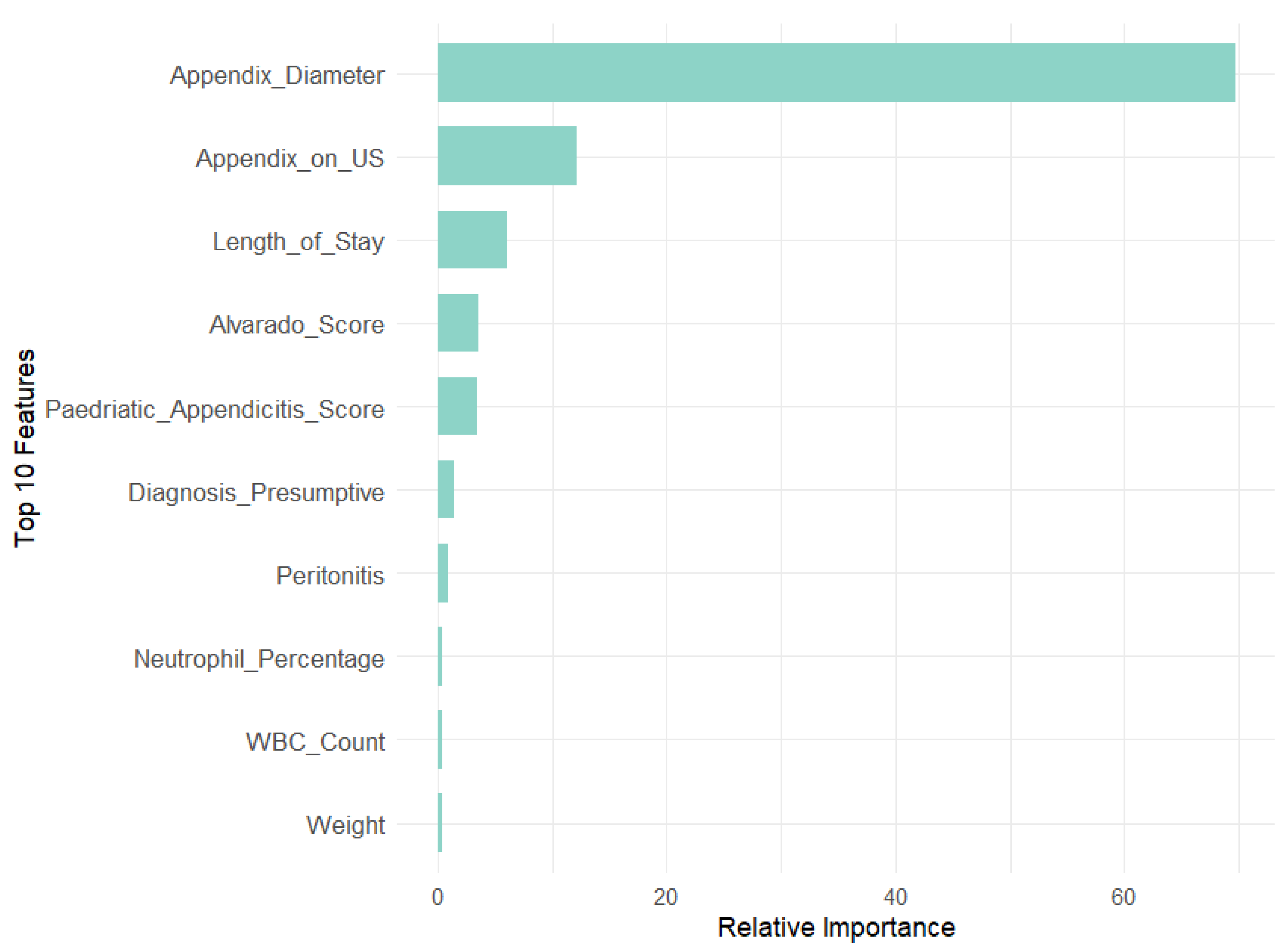
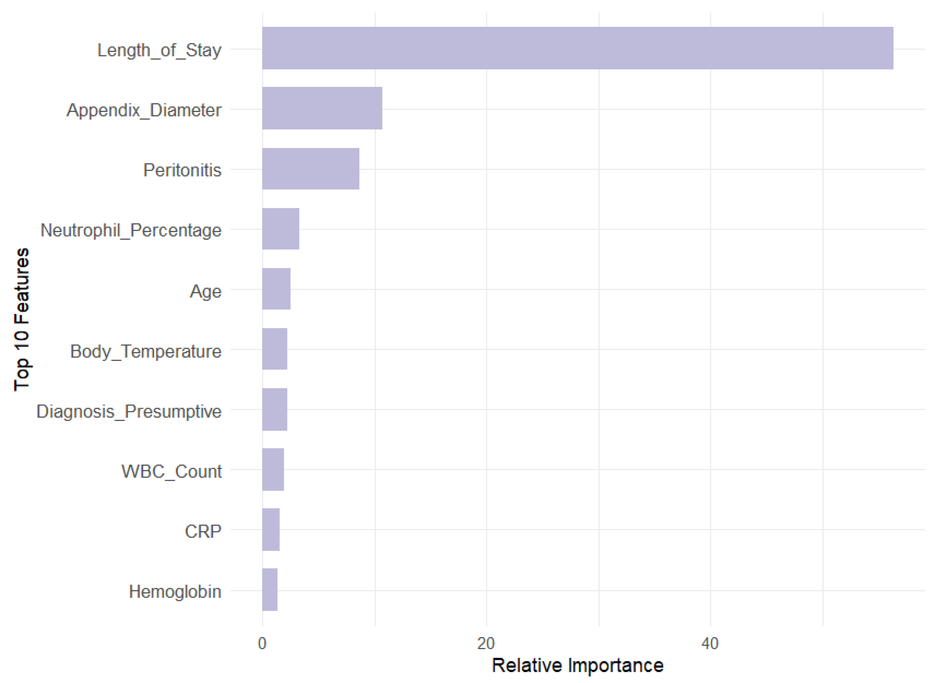
• GBM captures complex interactions between features and assesses feature importance based on their cumulative contribution across all boosting rounds, evaluated through relative importance (RI).

Our analysis revealed that appendix diameter is the most influential feature across all target variables in both models. It showed the highest Mean Decrease in Gini (147.71) and a substantial relative importance (69.73) for the Diagnosis target. Length of stay is also a significant predictor for Management (MDG = 104.79, RI = 55.44) and Severity (MDG = 74.34, RI = 57.83). In contrast, features like WBC count and neutrophil percentage are prominent in RF across all targets but exhibit lower relative importance in GBM, especially for Diagnosis (RI = 0.46 and 0.48, respectively). This suggests that GBM may underemphasize these features compared with RF. Additionally, peritonitis is moderately important in RF for Management (MDG = 38.31) but less significant in GBM (RI = 8.64).

Overall, RF highlights a broader range of important features, while gradient boosting machines focus on fewer features with higher relative importance. This contrast underscores the complementary strengths of these models: RF provides a wider array of significant predictors, whereas GBM emphasizes a few key variables with greater impact.

4.7. Models Parameters

Table 1. Summary of model parameters used in the experiments.

Model	Parameters
LR	NA
RF	- ntree: Number of trees (default = 100) - mtry: Number of features per split
XGBoost	- max_depth: Maximum tree depth (default = 6) - eta: Learning rate (default = 0.1) - nrounds: Number of boosting rounds (default = 100)
MLP	- size: Number of units in hidden layer (default = 5) - decay: Weight decay for regularization (default = 0.1) - maxit: Maximum iterations (default = 200)

summarizes the key parameters used for each model. For logistic regression, no explicit hyperparameter tuning was required as the model was used with its default settings. In the case of random forest, the number of trees (‘ntree’) was set to 100 to strike a balance between performance and computational efficiency, while the number of features per split (‘mtry’) followed the standard heuristic of the square root of the total number of features. For XGBoost, the tree depth (‘max_depth’) was fixed at six to prevent overfitting while maintaining sufficient model complexity, and the learning rate (‘eta’) was set to 0.1 to ensure stable convergence. The number of boosting rounds (‘nrounds’) was determined through cross-validation, selecting a value of 100 based on optimal performance. For the Multilayer Perceptron, the number of hidden units (‘size’) was set to five after testing different values to prevent overfitting while preserving expressiveness, and the regularization weight (‘decay’) was introduced to improve generalization. The maximum number of iterations (‘maxit’) was set to 200 to allow sufficient training without excessive computational cost. These choices were informed by prior research, standard heuristics, and empirical evaluation, ensuring a trade-off between accuracy, interpretability, and efficiency.

The choice of models in the experiments reflects a well-considered approach to addressing the complexities of diagnosing pediatric appendicitis, given the need for both predictive accuracy and interpretability. LR was chosen as a foundational model due to its simplicity and effectiveness in binary classification problems, particularly in healthcare contexts where model interpretability is crucial. LR allows for clear insights into the influence of individual predictors, which is useful for clinicians needing to understand the relationship between clinical features and appendicitis diagnosis.

RFs were included because they offer a robust ensemble approach, capable of capturing complex relationships between features without overfitting, which is critical when dealing with potentially noisy medical data. The RF algorithm is particularly well-suited for datasets with many features, as it can handle high-dimensional spaces efficiently and produce reliable predictions. Moreover, the use of feature importance scores from the RF model adds another layer of interpretability, allowing the identification of the most relevant predictors for diagnosing appendicitis.

The inclusion of XGBoost demonstrates a commitment to maximizing predictive performance. XGBoost has become a popular model in ML due to its ability to handle a wide range of data types and its effectiveness in boosting weak learners to create strong, accurate models. In the context of this study, XGBoost was selected for its ability to optimize performance through hyperparameters such as learning rate and tree depth, making it particularly useful for refining predictions in a complex clinical dataset where nuanced decision boundaries are needed to differentiate between cases.

MLPs are known for their ability to model highly non-linear relationships, which may exist in complex medical datasets. While MLPs are often less interpretable than other models like LR or RFs, their capacity for handling intricate patterns in data makes them valuable in cases where traditional models may fall short. In this study, the MLP was employed to assess whether techniques based on neural networks could further enhance diagnostic precision, particularly in instances where other models might struggle to capture complex interactions between clinical features.

Other models could have been considered. However, they were ultimately not chosen due to various limitations that made them less suitable for the task at hand. For instance, Support Vector Machines (SVMs) are known for their robust performance in classification tasks, especially when dealing with complex boundaries between classes. While SVMs work well with smaller datasets and can handle non-linear relationships through kernel functions, they can be difficult to interpret, which is a crucial factor in clinical settings where the transparency of the decision-making process is valued. The need to balance interpretability with predictive power meant that SVM was not ideal for this study.

4.8. Model Train and Evaluation

This section details the process of preparing the dataset for model training and evaluation, focusing on feature selection, data splitting, and model optimization.

Data preparation involved encoding categorical variables as binary targets, ensuring consistent factor levels between training and testing sets, and defining feature subsets based on their relevance to the prediction task.

Key features identified through Recursive Feature Elimination (RFE) were organized into specific subsets, including Demographic and Morphological variables, Clinical Scoring and Historical features, Laboratory Tests and Imaging variables, Clinical Symptoms and Physical Observations features, and a Literature-Based group that incorporated insights from recent studies. After the feature selection process, the Diagnosis model included 19 features, the Management model used 31 features, and the Severity model was trained with 11 features. The models deployed were LR, RF, XGB, and MLP, and each model was trained with these tailored feature subsets for the specific target variables.

The models’ performance was assessed using confusion matrices, ROC curves, and AUC scores, providing a detailed analysis of their effectiveness. LR served as a baseline model due to its simplicity and interpretability, while RF and XGB offered greater power for capturing non-linear relationships and complex feature interactions. MLPs were tested for their ability to further improve performance through advanced pattern recognition. An SVM model was also evaluated but ultimately removed from the experiments due to issues with handling factor levels for the Management target.

Our findings demonstrated high AUC, accuracy, sensitivity, and specificity across these models, indicating that they effectively captured patterns in the data and met the project’s analytical goals. Key performance metrics from the experiments underscored the robustness of these algorithms, which successfully addressed the complexities of our clinical dataset and managed the mixed data types effectively. Given the success of these models, we concluded that additional, newer algorithms were unlikely to add substantial performance improvements without complicating interpretability.

We also observed that feature selection significantly impacted model performance across the different targets. For Diagnosis and Management, a larger feature set (19 and 31, respectively) contributed to greater model accuracy (96.93% and 91.95%) and Kappa values (0.9363 and 0.8340), aligning with the complexity of these tasks. Conversely, Severity was accurately predicted with a more focused subset of 11 variables, reflecting the specialized nature of this classification. This targeted approach to feature selection effectively optimized model performance, balancing accuracy and interpretability across all tasks.

To further validate the feature selection process, we compared the MDG and RI scores of excluded versus retained features, particularly metabolic and environmental factors. Results consistently showed lower importance scores for excluded features, reinforcing the robustness of our RFE-driven selection process. For the Diagnosis target, high-impact variables like appendix diameter (MDG = 147.71, RI = 69.73) greatly outperformed metabolic factors like WBC count (MDG = 20.66, RI = 0.46) and neutrophil percentage (MDG = 15.26, RI = 0.48), as well as environmental factors like age (MDG = 9.93, RI = 0.37) and BMI (MDG = 9.27, RI = 0.14). In the Management target, length of stay (MDG = 104.79, RI = 56.44) and appendix diameter (MDG = 51.22, RI = 10.75) similarly outweighed metabolic predictors like hemoglobin (MDG = 8.14, RI = 1.32) and environmental ones like body temperature (MDG = 11.02, RI = 0.25). Lastly, for Severity, dominant features such as length of stay (MDG = 74.34, RI = 57.83) and CRP (MDG = 34.10, RI = 14.45) far surpassed BMI (MDG = 10.40, RI = 3.01) and weight (MDG = 9.05, RI = 1.89).

These findings confirm that excluded metabolic and environmental factors have minimal impact on predictive accuracy, ensuring that retained variables represent the most critical predictors.

4.9. Model Comparison by Target Variable

The performance of the selected ML models was compared across three target variables, as shown in Figure 9. The analysis involved extracting and evaluating key metrics, including AUC, accuracy, sensitivity, and specificity, across various feature subsets to identify the most effective combinations for each target.

For the Diagnosis target, LR, RF, and XGBoost models demonstrated superior discriminative power when using Laboratory and Imaging features, with AUCs reaching up to 0.9868 and accuracies around 94%. In contrast, models based on Demographic and Morphological features consistently underperformed, with AUCs as low as 0.5131 and accuracies just above 50%. MLPs further underscored the effectiveness of Laboratory and Imaging, and Literature-derived features in accurate diagnosis.

In the Management context, Clinical Symptoms and Observations, along with Literature-Based features, achieved the highest predictive accuracy across all models, with AUCs ranging from 0.9434 to 0.9596 and accuracies close to 90%. These features enabled robust discrimination between conservative and surgical management approaches. While Laboratory and Imaging features also performed well, with AUCs around 0.877 and accuracies of 80–83%, they were slightly less effective compared with the top-performing subsets. Demographic and Morphological features exhibited poor discriminative power, with AUCs between 0.4962 and 0.5867.

For Severity classification, models performed best using Literature-Based and Clinical Symptoms and Observations features, achieving near-perfect AUCs of 0.9986 and demonstrating strong sensitivity and specificity. LR, RF, XGBoost, and MLPs all highlighted these features as critical for accurate severity prediction. Conversely, Demographic and Morphological features were notably less effective, yielding AUCs as low as 0.4642, underscoring their limited utility in distinguishing severe from non-severe cases.

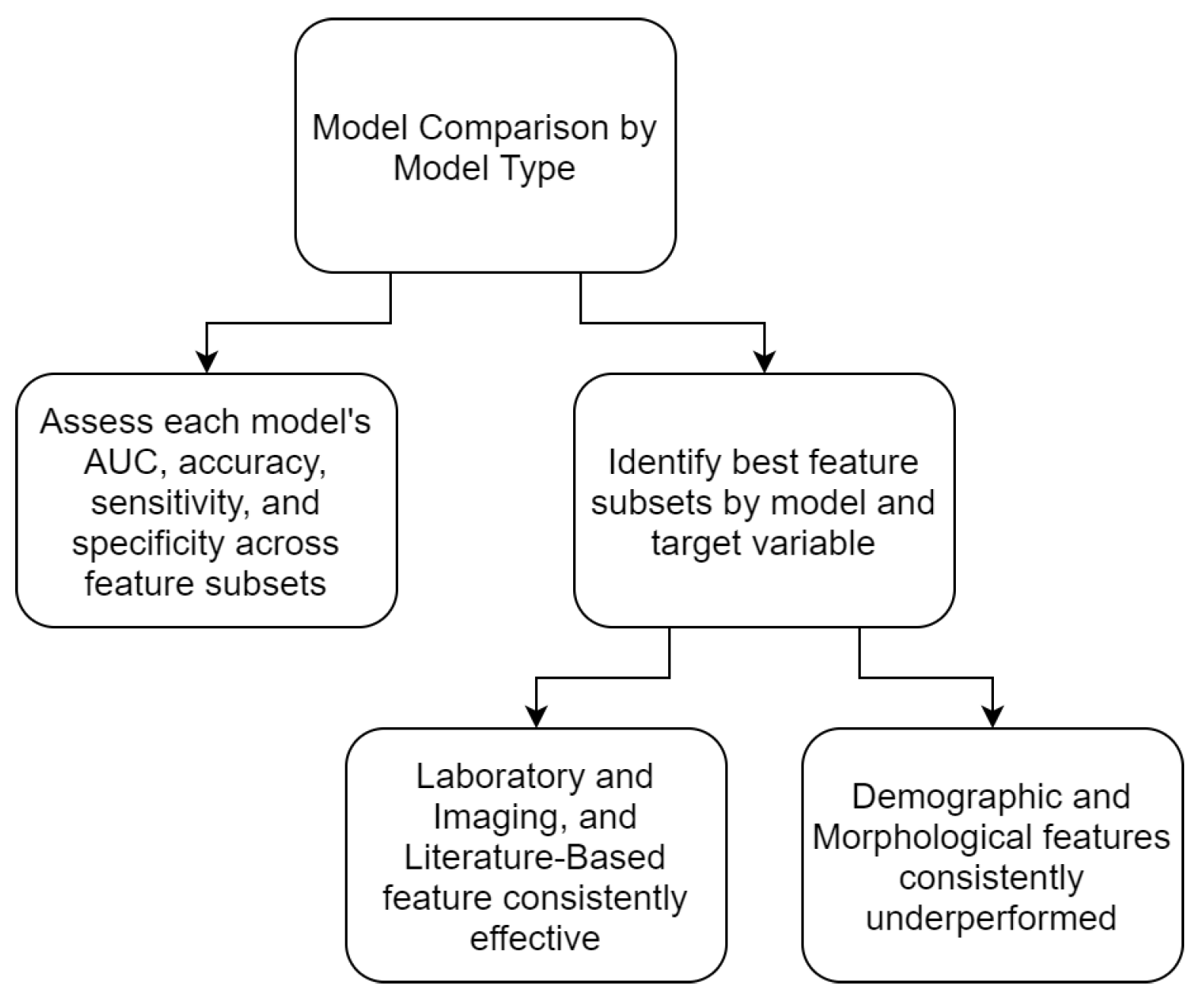
Overall, Laboratory and Imaging and Literature-Based feature sets consistently outperformed others across all three target variables, demonstrating their robustness and reliability. In contrast, Demographic and Morphological features consistently underperformed across all targets. The Clinical Symptoms and Observations feature set produced moderate to strong results depending on the target variable, reinforcing the need for careful feature selection in optimizing model performance.

4.10. Model Comparison by Model Type

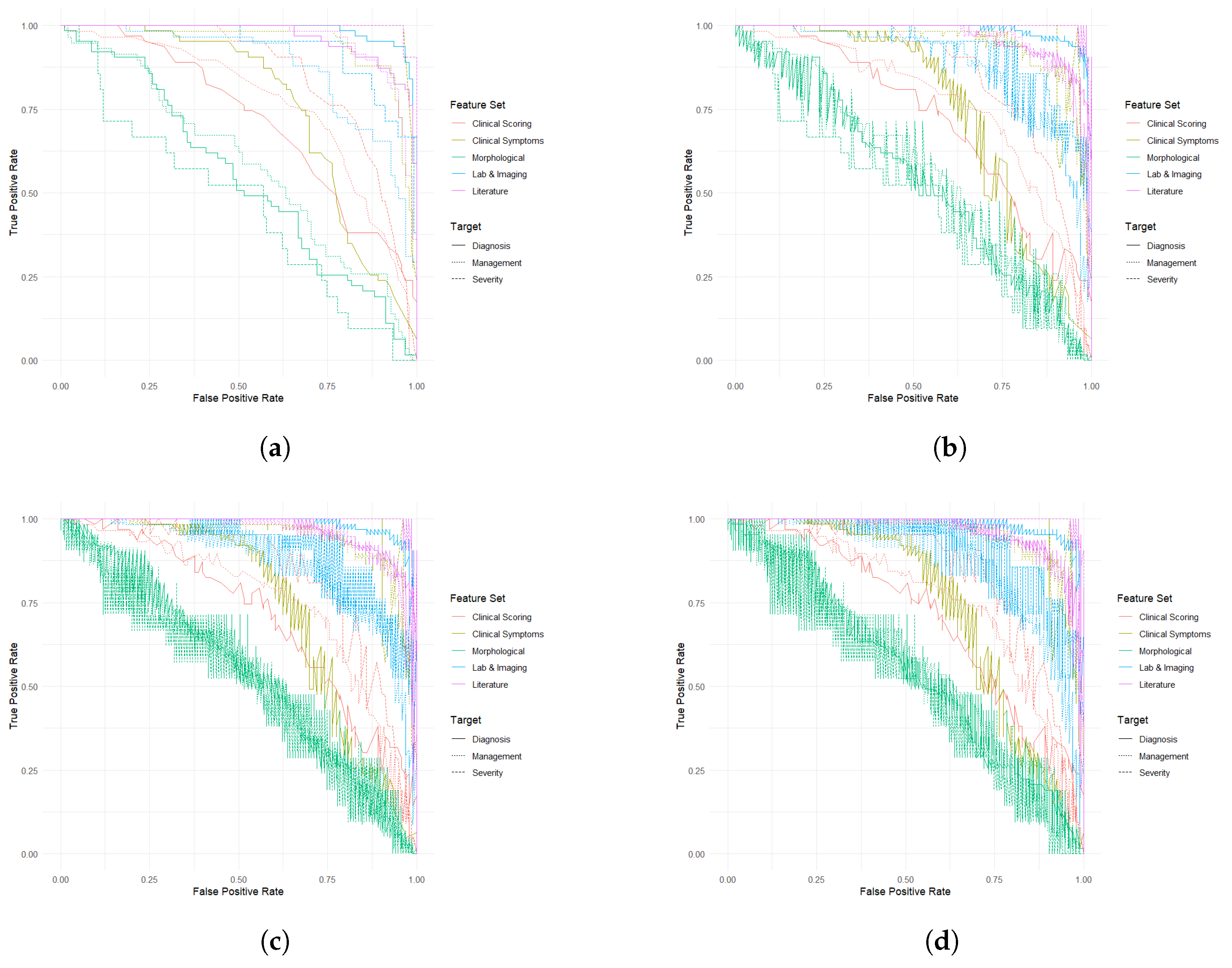
To thoroughly evaluate the performance of different ML models, as per Figure 10, we compared their effectiveness across three target variables using different feature subsets, as depicted in Figure 11. Key metrics, including AUC, accuracy, sensitivity, and specificity, were analyzed to determine the most effective feature combinations for each target.

For the Diagnosis target, all models exhibited superior performance with the Laboratory and Imaging and Literature-Based feature sets. LR and XGBoost reported similar AUC values for Laboratory and Imaging features (0.9862) and Literature features (0.9652), with RF also favoring these sets but with slightly different values (0.9868 and 0.9712, respectively). MLPs showed the highest AUCs for Laboratory and Imaging (0.9862) and Literature-Based features (0.9652). In contrast, models based on Demographic and Morphological features consistently underperformed, with the lowest AUC (0.5472) and accuracy (59.62%).

For Management, Clinical Symptoms and Observations and Literature-Based feature sets were notably effective across all models. LR and XGBoost achieved high AUCs of 0.9457 and 0.9585, respectively, for these feature sets. Similarly, RF ranked these features highly, though with slightly lower AUCs (0.9353 and 0.9596). The Demographic and Morphological feature set consistently performed poorly, reflecting its limited utility in predicting management strategies.

When predicting Severity, Literature-Based and Clinical Symptoms and Observations feature sets achieved the highest performance across all models. MLPs and XGBoost reported exceptional results for Literature-Based features, with AUCs of 0.9986 and 0.9965, respectively. LR and RF showed strong performance but with slightly lower AUC values compared with XGBoost and MLPs. Consistent with other targets, Demographic and Morphological features produced weaker results, particularly in distinguishing between severity levels.

One of the critical aspects of developing machine learning models for clinical applications is the careful selection of appropriate algorithms. In this study, we prioritized models that are well-suited for structured clinical data, including logistic regression (LR), random forest (RF), gradient boosting machines (GBMs), and Multilayer Perceptrons (MLPs). These models were chosen based on their ability to handle structured tabular data, their interpretability, and their established performance in medical decision support tasks.

The use of deep learning architectures such as Convolutional Neural Networks (CNNs) or Recurrent Neural Networks (RNNs) was considered; however, such models typically require significantly larger datasets with high-dimensional features, such as imaging or sequential data, to generalize effectively. Given that our dataset consists primarily of structured clinical variables rather than unstructured data, deep learning models were not the primary focus of this study. Moreover, deep architectures often demand extensive hyperparameter tuning and increased computational resources, which may not be optimal for real-time clinical decision support in resource-limited settings.

Support Vector Machines (SVMs) were also considered due to their strong theoretical foundation in high-dimensional classification problems. However, in preliminary experiments, SVMs exhibited computational inefficiencies, particularly with larger sample sizes and feature-rich datasets. Additionally, tree-based ensemble models such as RF and GBM provided superior interpretability, an essential factor in clinical decision-making, allowing the identification of key predictive features contributing to diagnostic accuracy.

The selection of machine learning models is ultimately guided by the trade-off between predictive performance, interpretability, and computational feasibility. The findings of this study reinforce the suitability of ensemble learning methods for structured clinical data while acknowledging the potential for deep learning in more complex, multi-modal datasets.

Another key aspect of this study was the rigorous feature selection process, which ensured that only the most relevant predictors were included in the machine learning models. However, as with any data-driven approach, preprocessing decisions, such as handling missing values, can introduce potential biases that warrant careful consideration. Missing data were handled using established imputation techniques, including mean imputation for continuous variables and mode imputation for categorical variables when appropriate. While these methods prevent data loss and allow for the inclusion of a larger sample size, they also assume that missingness is random (Missing Completely at Random, MCAR), which may not always hold in clinical datasets. If certain variables have systematic missingness (e.g., laboratory test results not being recorded for milder cases), the imputation strategy could introduce bias, particularly by underrepresenting specific patient subgroups. Another critical preprocessing step was outlier detection and removal, which helps improve model robustness but may also lead to the exclusion of rare but clinically significant cases. For example, extreme values in laboratory markers could correspond to severe cases of appendicitis, and their removal could influence model sensitivity in detecting such cases. To mitigate these potential biases, we performed sensitivity analyses, comparing model performance with and without imputed values to assess the impact of missing data handling. The results indicated that, while imputation slightly affected individual feature importance rankings, overall model performance remained stable, suggesting that the selected imputation strategy did not substantially alter the predictive capabilities of the models.

A further challenge consists of the interpretability of complex models such as random forest, XGBoost, and Multilayer Perceptron, which, despite their high predictive power, often function as black-box systems. Clinicians require transparent decision-making processes to trust and effectively utilize ML-based recommendations. To address this, future research should focus on integrating explainability techniques to provide insights into how these models weigh different clinical features.

Another significant challenge is the deployment of ML models into hospital systems. Electronic Health Records (EHR) systems vary across institutions, requiring seamless integration of ML models to ensure real-time decision support without disrupting clinical workflows. Technical barriers such as data standardization, interoperability between different EHR platforms, and computational infrastructure requirements must be addressed before these models can be effectively implemented in a clinical setting.

Additionally, the success of ML applications in healthcare depends not only on technical feasibility but also on clinical adoption and training. Many healthcare professionals may be unfamiliar with ML-based decision support tools, necessitating targeted training programs to improve their understanding of model predictions and limitations. Without adequate training, there is a risk of either over-reliance on ML outputs or outright rejection due to skepticism. Future implementations should consider collaborative frameworks between data scientists and clinicians to ensure usability, trust, and proper interpretation of ML-driven insights.

Finally, ethical and regulatory considerations must be taken into account, particularly regarding model validation, patient data privacy, and liability in ML-assisted decision-making. Regulatory bodies require robust validation studies before ML models can be deployed in routine practice, emphasizing the need for multicenter external validation to ensure fairness, safety, and efficacy across diverse patient populations.

5. Conclusions and Future Work

This work addressed the diagnostic challenges of pediatric appendicitis through the application of machine learning (ML) techniques to enhance both diagnostic accuracy and patient management. Pediatric appendicitis is complex to diagnose due to age-related symptom variations, communication barriers, and the absence of standardized diagnostic guidelines, especially for children under five. These factors, coupled with non-specific symptoms in younger children and females, often result in misdiagnoses, delayed treatments, and unnecessary surgical interventions.

Our findings demonstrated that ML algorithms—including logistic regression (LR), random forest (RF), XGBoost, and Multilayer Perceptron (MLP)—achieved high AUC and accuracy values, confirming their robustness and reliability. Consistent with clinical expectations, key symptoms such as neutrophilia, nausea, loss of appetite, coughing pain, and migratory pain, along with established literature-based features like the Alvarado Score, Pediatric Appendicitis Score, appendix diameter, C-reactive protein, and White Blood Cell count emerged as the most effective predictors across all targets. In contrast, demographic and morphological factors such as age, height, weight, and BMI were less predictive, reinforcing the clinical perspective that symptomatology and specific biomarkers provide more direct diagnostic insights compared with general physical characteristics.

The main contribution of this work is demonstrating how ML can complement clinical decision-making by providing precise, data-driven insights into pediatric appendicitis. This approach has the potential to reduce negative appendectomies, improve diagnostic precision, and inform treatment strategies, ultimately leading to better patient outcomes.

However, several limitations need to be addressed in future research. One key challenge is the incomplete nature of the dataset, particularly regarding ultrasound imaging and laboratory results, which may affect model performance and predictive accuracy. To improve model robustness, future research should focus on collecting more comprehensive, high-quality clinical and imaging data.

A critical next step is the external validation of the proposed models. While the models performed well on the current dataset, generalizability must be confirmed by validating them on independent datasets from diverse clinical settings. This would ensure that the models maintain their predictive accuracy across varying patient populations and institutional protocols. Moreover, multicenter validation studies would help mitigate biases introduced by a single data source. Future research should also explore domain adaptation techniques to fine-tune the models for different clinical environments while maintaining diagnostic accuracy. Additionally, interpretability remains a challenge for complex ML models such as RF and XGBoost. Although these models achieved high predictive accuracy, their complexity can hinder adoption in clinical practice. Future efforts should aim to improve model transparency using explainability tools such as SHAPs (Shapley Additive Explanations) and LIME (Local Interpretable Model-Agnostic Explanations) to facilitate their integration into clinical workflows.

Lastly, exploring novel predictors, such as emerging biomarkers, genetic information, and detailed patient histories, may further enhance diagnostic accuracy, particularly in atypical cases. Future research should also investigate the ethical implications of ML-driven diagnostics, ensuring that AI applications in pediatric healthcare remain transparent, equitable, and aligned with clinical standards.

By addressing these challenges, future studies can advance the reliability and applicability of ML models in pediatric appendicitis diagnosis, paving the way for AI-assisted decision support tools that optimize patient care.