Distributed Denial of Service Attack Detection in Software-Defined Networks Using Decision Tree Algorithms

Abstract

A software-defined network (SDN) is a new architecture approach for constructing and maintaining networks with the main goal of making the network open and programmable. This allows the achievement of specific network behavior by updating and installing software, instead of making physical changes to the network. Thus, SDNs allow far more flexibility and maintainability compared to conventional device-dependent architectures. Unfortunately, like their predecessors, SDNs are prone to distributed denial of service (DDoS) attacks. These attack paralyze networks by flooding the controller with bogus requests. The answer to this problem is to ignore machines in the network sending these requests. This can be achieved by incorporating classification algorithms that can distinguish between genuine and bogus requests. There is abundant literature on the application of such algorithms on conventional networks. However, because SDNs are relatively new, they lack such abundance both in terms of novel algorithms and effective datasets when it comes to DDoS attack detection. To address these issues, the present study analyzes several variants of the decision tree algorithm for detection of DDoS attacks while using two recently proposed datasets for SDNs. The study finds that a decision tree constructed with a hill climbing approach, termed the greedy decision tree, iteratively adds features on the basis of model performance and provides a simpler and more effective strategy for the detection of DDoS attacks in SDNs when compared with recently proposed schemes in the literature. Furthermore, stability analysis of the greedy decision tree provides useful insights about the performance of the algorithm. One edge that greedy decision tree has over several other methods is its enhanced interpretability in conjunction with higher accuracy.

1. Introduction

The issue of developing and maintaining security in a computer network has always remained a primary issue for the efficient functioning of the network [1,2]. With the advent of modern paradigms such as cloud computing and IoT, the importance of maintaining security has become the most prominent issue [3,4]. Traditionally, security has been implemented at both the software and hardware levels. More specifically, the data plane can be accessed via the control plane. However, the control plane consists of several hardware devices, such as switches and routers, as well as firewalls. These devices run complex protocols and operating systems or firmware to efficiently perform their tasks [5]. Handling of these devices is a difficult task due to non-compliance of conventions by hardware vendors, inconsistencies in policies, and scalability issues. These complexities are quite challenging and result in network management and performance issues. The answer is to redefine networking to support more protocols and applications by having a network paradigm where network controls are programmable. SDNs fulfill these requirements with simple, easy, and effective networking.

In an SDN, the entire network is logically centralized through a network operating system (NOS). The NOS acts as a layer between the forwarding devices and network applications. The former consists of hardware devices, while the latter is software designed to enforce particular behavior on the network (see Figure 1). In other words, the operating system acts as a layer between different types of software and the hardware required to run that software. However, this centralization leads to higher vulnerability to DDoS attacks. The DDoS attack is basically a flood of bogus requests which confines the network traffic, thus immobilizing the network. The attack is usually done via bots, which can be computers or other IoT devices set to go off at a particular time. A diagrammatic representation of the architecture of DDoS attack is given in Figure 2. To understand the magnitude, Amazon was hit by a DDoS attack on the scale of 2.3 Tbps in the first quarter of 2020 [6]. For an organization that operates 24/7 across the globe, such attacks have severe financial repercussions.

Due to the vulnerability of SDNs, a notable amount of research has been carried out in the past few years with regard to the use of machine learning (ML) and deep learning (DL) for DDoS attack detection [8]. The well-known techniques used by researchers for the DDoS detection problem include K-nearest neighbors (KNN), decision tree (DT), ensemble learning (EL), random forest (RF), support vector machine (SVM), and artificial neural networks (ANNs). A detailed discussion of these algorithms can be found in Nadeem et al. [9].

Table 1. Summary of previous studies on the use of ML/DL algorithms for DDoS attack detection in SDN.

Reference	Year	Algorithms	Datasets
[15]	2018	SVM, DNN	KDD-Cup99, Mininet for SDN
[16]	2018	SVM	KDD-Cup99
[11]	2019	SVM, MLP, DT (CART), RF	Scapy tool, Mininet
[30]	2019	DT (J48), RF, SVM, KNN	hping
[32]	2020	SVM (linear, polynomial)	Scapy tool
[33]	2020	K-means++, RF	InSDN
[24]	2020	DNN, linear SVM, DT, NB	CICIDS2018
[34]	2020	CNN-LSTM, MLP, SVM	Self-generated
[2]	2020	KNN, NB, AdaBoost, DT, RF, rbf-SVM, lin SVM, MLP	InSDN (self-generated)
[35]	2021	RNN, LSTM, GRU	InSDN
[25]	2021	KNN, SVM, DT, NB, RF, XGBoost	CIC-DDoS2019
[17]	2021	SVM, DT	KDD-Cup99
[1]	2021	SVC-RF, LR, SVC, KNN, RF, ANN	New dataset
[18]	2022	KNN, logistic regression, DT	KDD-Cup99
[19]	2022	SVM, GLM, NB, DA, FNN, DT, KNN, BT	1999 DARPA, InSDN, DASD
[36]	2022	LR, NB, DT	Mininet for SDN
[26]	2022	RF, KNN-SVM, NB	CIC-DDoS2019
[20]	2022	SVM (Ensemble), DT (J48), KNN	KDD-Cup99
[9]	2022	SVM, KNN, NB, RF and DT	NSL-KDD
[27]	2022	PCA, KPCA, LDA, DT, RF	CIC-DDoS2019
[37]	2023	SVM, NB, MLP	Mininet
[38]	2023	SVM, DT, Gaussian NB, RF, extra tree classifier, ANN	Mininet
[21]	2023	RNN, GRU, MLP, LSTM	CICIDS2017, CIC-DDoS2019
[22]	2023	GRU, hybrid DL	CICIDS2017, NSL-KDD
[39]	2024	LR, LDA, NB, KNN, CART, AdaBoost, RF, SVM	InSDN
[23]	2024	KNN	CICIDS2017, CICIDS2018, CIC-DDoS2019
[28]	2024	MLP	CIC-DDoS2019
[31]	2024	XGBoost-SHAP	CIC-IOT-2023
[40]	2024	SVM, random forest, KNN	Dataset by Ahuja et al. [1]
[29]	2025	SHAP, CNN-BiLSTM, AE-MLP, CNN-MLP	InSDN, CIC-DDoS2019

presents a summary of several recent studies. One obvious limitation that is highlighted by the summary regards to the datasets used; there are no viable or realistic datasets that are particularly developed for SDN attacks, and the datasets developed by individual researchers are also not available publicly, and hence cannot be used for benchmarking. These observations are also confirmed by several past studies [10,11,12,13,14]. For example, studies have used general datasets such as KDD-Cup99 [15,16,17,18,19,20], CICIDS 2017 [21,22,23], CICIDS 2018 [23,24], CIC-DDoS 2019 [21,23,25,26,27,28,29], and others [9,22,30,31]. Furthermore, although several studies [1,2,11,15,19,32,33,34,35,36,37,38,39,40] have used SDN-specific datasets, there are only two reported studies that have made their comprehensive dataset available in the public domain. The first is the InSDN dataset proposed by Elsayed et al. [2], which has been used in other studies [29,33,35,39]. The second dataset was proposed recently by Ahuja et al. [1], who carried out an in-depth analysis of DDoS attack detection in SDNs using their proposed dataset.

Another observation in Table 1 is that most studies performed a comparative analysis of various ML and DL algorithms, where the focus was to mutually compare conventional algorithms and report the results using well-known performance measures such as accuracy, precision, recall, and F-score. Although such comparative studies give useful insight into the problem, they did not place emphasis on algorithmic improvement or provide further analysis beyond the use of traditional performance measures. Among all studies reported in Table 1, there are only a few that proposed or analyzed advanced ML/DL algorithms (such as hybrid or ensemble algorithms). For example, Firdaus et al. [33] proposed a modified version of the the K-means algorithm, termed K-means++, and evaluated its performance using the InSDN dataset. Similarly, Nugraha et al. [34] proposed a CNN–LSTM hybrid and analyzed its performance using a custom-generated dataset. Karki et al. [26] and Revathi et al. [20] proposed SVM ensembles and assessed the performance of their proposed algorithms using the CICIDS2019 and KDDCup-99 datasets, respectively. Finally, Elubeyd et al. [22] proposed a hybrid deep learning algorithm that was evaluated on the CICIDS2017 and NSL-KDD datasets. It should be noted that while the aforementioned studies proposed new variants of ML/DL algorithms, all of them, with the exception of Firdaus et al. [33], used datasets that did not qualify for testing SDN-based attack detections.

As observed in the above discussion, it turns out that there are only two studies by Ahuja et al. [1] and Elsayed et al. [2] where SDN-specific datasets were developed that are available in the public domain. In addition, both Ahuja et al. [1] and Elsayed et al. [2] proposed advanced/hybrid variants of existing ML/DL algorithms, which gave better results than the existing basic ML/DL methods. Ahuja et al. [1], using their own dataset, achieved an accuracy of 98.8% and a very good false alarm rate of 0.02%. For similar reasons, Elsayed et al. [2] also generated their own dataset. For multiple types of attacks, both datasets are not balanced, but the algorithms that they devised for automated detection of these attacks give good results. The present study focuses on the reasons behind the difference in the results, and also on proposing a slightly different technique to solve the problem of DDoS attack detections on SDNs.

One strong motivation behind the present study is to build on preliminary work carried out in a recent study by Haq et al. [40], and to improve the results of the evaluation criteria using a simpler algorithm; an algorithm that does not rely too much on randomness, as is the case with several algorithms used in the past studies (such as the RF classifiers). The study by Haq et al. [40] employed three ML algorithms, namely SVM, RF, and KNN, while using the dataset of Ahuja et al. [1] without any focus on algorithm modification or proposing better variants of any of the three algorithms. In addition, hyperparameter tuning of feature selection was not considered. Furthermore, Haq et al. neither conducted any experiments for validation of the constructed models nor checked whether variation in accuracy metrics occurs when the data is changed. Their study also did not make a comparative analysis with previous studies.

The present study is significantly different from the work of Haq et al. [40] and demonstrates several novel aspects (as identified in Section 3). The present study aims to show that removing certain preprocessing steps can lead to improvement in accuracy, especially in the case of the dataset generated by Ahuja et al. [1]. The model constructed in the present study is more interpretable, uses k-fold and Monte Carlo validations, and provides results with stratified as well as unstratified data, in contrast to Haq et al. Furthermore, since the datasets by Ahuja et al. [1] and Elsayed et al. [2] used in the present study have different features and different numbers of features, this study also shows that the approach of incrementally constructing a decision tree is generalizable over different datasets. As such, the discussion in Section 2 summarizes the work done by Ahuja et al. [1] and Elsayed et al. [2] while identifying their strengths and weaknesses.

The rest of the paper is organized as follows. Section 2 provides a brief overview of the two core studies whose datasets have been used in the present study. This is followed by Section 3, which highlights the novelty and contributions of the proposed work. The proposed approach is presented in Section 4. The performance measures used in the study are described in Section 5. Results and discussion are provided in Section 6. The limitations of the proposed approach are identified in Section 7. The paper concludes and identifies directions for future research in Section 8.

2. Background and Description of Datasets

This section discusses the details of the two datasets used in the present study, highlighting the key aspects as well as the limitations of the studies by Ahuja et al. [1] and Elsayed et al. [2] A brief description of the two datasets and their attributes is also provided.

2.1. The Study of Ahuja et al. [1]

In the work by Ahuja et al. [1], a simulated dataset was developed using the Mininet emulator and made publicly available on the Mendeley repository. The major work by Ahuja et al. [1] was the identification of novel features for DDoS attack detection. The original dataset contains a total of 104,345 instances, where each instance is comprised of 23 features before preprocessing.

Table 2. Number of instances in the Ahuja et al. dataset [1].

Traffic Class	Number of Instances
Benign	63,561
Malicious	40,784
TCP	29,436 (18,897 benign, 10,539 malicious)
UDP	33,588 (22,772 benign, 10,816 malicious)
ICMP	41,321 (24,957 benign, 16,364 malicious)

provides the details of these instances, while

Table 3. Features used in the study of Ahuja et al. [1].

No.	Feature	Description
1	dt	Date and time
2	switch	Datapath ID of the switch in the topology
3	src	Source IP address of the flow
4	dst	Destination IP address of the flow
5	pktcount	Number of packets sent during the flow
6	bytecount	Number of bytes sent during the flow
7	dur	Duration of the flow in seconds
8	dur_nsec	Duration of the flow in nanoseconds
9	tot_dur	Total duration of the flow in nanoseconds
10	flows	Total number of flows in the switch
11	packetins	Number of packet_in messages to the controller
12	pktperflow	Packet count per flow
13	byteperflow	Byte count per flow
14	pktrate	Packet rate calculated using packet counts
15	Pairflow	Boolean value
16	Protocol	Protocol associated with the traffic flow
17	port_no	Port number of the switch
18	tx_bytes	Number of bytes transmitted on the port
19	rx_bytes	Number of bytes received on the port
20	tx_kbps	Transmit bandwidth of the port
21	rx_kbps	Receive bandwidth of the port
22	tot_kbps	Total bandwidth of the port
23	label	The label of the attack

shows the features identified in Ahuja et al. [1].

It is mentioned in Ahuja et al. [1] that after preprocessing and including dummy variables for categorical features, the data increased from 23 to 67 features, and that RF produced excellent results with a large number of features. This step implies that encoding was used (as mentioned by Potdar et al. [41]) so that categorical features could be given as input to classifiers that work only on numerical data (like linear regression, SVC, NNet). PCA (principal component analysis) was implemented on the resultant dataset, compressing it to only 20 features. After the application of PCA on the data, t-SNE (t-distributed stochastic neighborhood embedding) was applied, further compressing the dataset from 20 features to 2 features. These two features are then used by a SVC (support vector classifier) to classify the data, but some of the points are situated in such a way that they lie in more than one class. These points are then given as input to an RF classifier for a more accurate prediction.

From the literature review performed, the work of Ahuja et al. [1] stands out in the sense that this paper used an ensemble technique for DDoS detection. Therefore, an in-depth analysis was performed on the steps taken by Ahuja et al. [1] to identify possible gaps. Hancock et al. [42] pointed out that the distance between any two pairs is the same. Another disadvantage of this type of encoding is the extra use of resources to represent information. In the case of Ahuja et al. [1], it resulted in four times the number of features than the original dataset. In addition, applying encoding can lead to good results with DL, as shown by Hancock et al. [42] and Duan et al. [43], but DL has the drawback of being a black box.

Furthermore, Trunk et al. [44] show that as the dimensionality increases, the accuracy of a model decreases. Wheeler [45] shows how applying one-hot encoding before PCA is counterintuitive. Ghosh et al. [46] explains that instead of using PCA, which results in a difficult solution space for neural nets to converge in, one can use another variant of PCA, namely nonlinear PCA, which is discussed in detail by Linting et al. [47].

In addition to the above discussion on the application of PCA to the given dataset, the next step is to critically analyze the application of t-SNE to the problem in question. Maaten and Hinton [48] proposed an algorithm called t-SNE, which works by mapping the neighbors of each data point in terms of probability of neighborhood. As mentioned in this section earlier, the use of t-SNE reduced the number of features to two. However, Xu et al. [49] discusses why t-SNE should not itself be used for classification. Vidyala [50] explains that t-SNE should not be used after applying PCA, as was done by Ahuja et al. [1]. Furthermore, Shah et al. [51] show that applying t-SNE does not preserve the desired clustering. This point was further elaborated by Waagen et al. [52] by showing how t-SNE does not preserve the local and global structure of the actual dataset after transformation. However, Ahuja et al. [1] show good results, forcing one to conclude that these results can be further improved using other techniques.

2.2. The Study of Elsayed et al. [2]

The second established dataset, termed InSDN, was created by Elsayed et al. [2]. What makes their work stand out is the fact that instead of only focusing on DDoS attacks for SDNs, their dataset also incorporated several other attacks, namely DoS, web attacks, R2L, malware, probe, and U2R. The dataset consists of 343,939 instances comprised of normal and attack traffic. Of these, 68,424 instances are classified as normal, and 275,515 instances are categorized as attack. They divided the dataset into three groups based on the traffic types and the target machines. The first group includes normal traffic only. In the second group, attack traffic that targets the Metasploitable-2 server is considered. The last group contains attacks on the OVS machine [2].

Table 4. Number of instances in the Elsayed et al. dataset [2].

Data Group	Number of Instances	Percentage
Normal	68,424	19.9%
Metasploitable-2	136,743	39.76%
OVS	138,772	40.34%

provides the distribution of the instances in each group. Furthermore, in the original dataset, 77 features were identified. Of these, 48 features were selected.

Table 5. Attributes used in the study of Elsayed et al. [2].

No.	Attribute Name	No.	Attribute Name
1	Protocol	25	Fwd-IAT-Min
2	Flow-duration	26	Bwd-IAT-Tot
3	Tot-Fwd-pkts	27	Bwd-IAT-Mean
4	Tot-Bwd-Pkts	28	Bwd-IAT-Std
5	TotLen-Fwd-Pkts	29	Bwd-IAT-Max
6	TotLen-Bwd-Pkts	30	Bwd-IAT-Min
7	Fwd-Pkt-Len-Max	31	Fwd-Header-Len
8	Fwd-Pkt-Len-Min	32	Bwd-Header-Len
9	Fwd-Pkt-Len-Mean	33	Fwd-Pkts/s
10	Fwd-Pkt-Len-Std	34	Bwd-Pkts/s
11	Bwd-Pkt-Len-Max	35	Pkt-Len-Min
12	Bwd-Pkt-Len-Min	36	Pkt-Len-Max
13	Bwd-Pkt-Len-Mean	37	Pkt-Len-Mean
14	Bwd-Pkt-Len-Std	38	Pkt-Len-Std
15	Flow-Bytes/s	39	Pkt-Len-Var
16	Flow-Pkts/s	40	Pkt-Size-Avg
17	Flow-IAT-Mean	41	Active-Mean
18	Flow-IAT-Std	42	Active-Std
19	Flow-IAT-Max	43	Active-Max
20	Flow-IAT-Min	44	Active-Min
21	Fwd-IAT-Tot	45	Idle-Mean
22	Fwd-IAT-Mean	46	Idle-Std
23	Fwd-IAT-Std	47	Idle-Max
24	Fwd-IAT-Max	48	Idle-Min

describes the features in this dataset.

Like Ahuja et al., Elsayed et al. [1,2] also used some standard ensemble techniques like AdaBoost, rbf-SVM and lin-SVM, and RF classifier. However, the results showed that the accuracy achieved by these techniques, with the exception of RF, was less than that achieved by simple ML algorithms like naive Bayes, KNN, DTs, and multi-layer perceptron (MLP). The most promising results were achieved by the RF classifier. Even though RF showed promising results, the problem with RFs, like most ensemble techniques, is that they require a grid search of the hyperparameters (such as number of trees) to consider, the tree depth, and the number of features to consider for a split. Furthermore, the study of Elsayed et al. [2]. does not mention the encoding techniques incorporated for categorical variables, which would have been necessary for techniques like linear regression, radial basis function networks, SVMs, and MLP.

3. Novelty and Contributions

Recent studies [53,54] show that simulated datasets used for attack detection usually yield high accuracy. However, their implementation in a real environment does not give the same level of accuracy. This is due to the patterns of values that are not present in the simulated dataset. Thus, it is of extreme importance to adjust the model in accordance with the real-world environment. The problem with most advanced ML models is that these models are not interpretable enough to allow the user to infer the relationship between feature values and classifications [55]. In the case of Ahuja et al. [1], the best accuracy was achieved by first implementing SVCs and then applying RF. SVCs are not easily interpretable [56]. Elsayed et al. [2] achieve excellent results via RF classifiers, which are interpretable but not as interpretable as single DTs, as RF classifiers pose the problem of multiple tree aggregation [57]. Therefore, what is most desirable is an easily interpretable model [58], whose functionality can be understood in the field environment. This is the direction that the approach proposed in the present study has taken.

As mentioned earlier, the preliminary work by Haq et al. [40] provided limited insights about DDoS attack detection in SDNs through a basic analysis on the impact of feature selection in the context of the problem. The study only used a single dataset, and without providing any comparison with other works reported in the literature or improvement in existing core techniques.

The key limitations of the two core studies by Ahuja et al. [1] and Elsayed et al. [2] have been highlighted above. Keeping in view these observations and the above discussion, the novel aspects and key contributions of the present study are enumerated as follows:

• In the past studies on the detection of DDoS attacks, SDN-specific datasets were not available or not utilized. As such, the main focus in those studies was the creation of datasets. In the present study, our contribution is in utilizing two recent and core datasets for the underyling problem while utilizing a decision-tree-based approach. The availability of two datasets has enabled us to verify that the detection of malicious and benign network traffic is closer to how it appears in reality, as opposed to being biased towards how it is represented in a single dataset.
• The previous technique by Ahuja et al. [1] had multiple steps involved, which increased the complexity of the overall algorithm. In the technique proposed herein, certain algorithmic layers and encoding techniques have been removed altogether, and there is no implementation of t-SNE (see details in the next section). This removal results in the proposed approach being simpler. Furthermore, Elsayed et al. [2] applied RF directly to their dataset, but random forest requires certain parameters’ selection, which leads to a grid search for optimization. Our contribution is in proposing a technique that avoids the above issues, leading to a simpler and time-efficient approach.
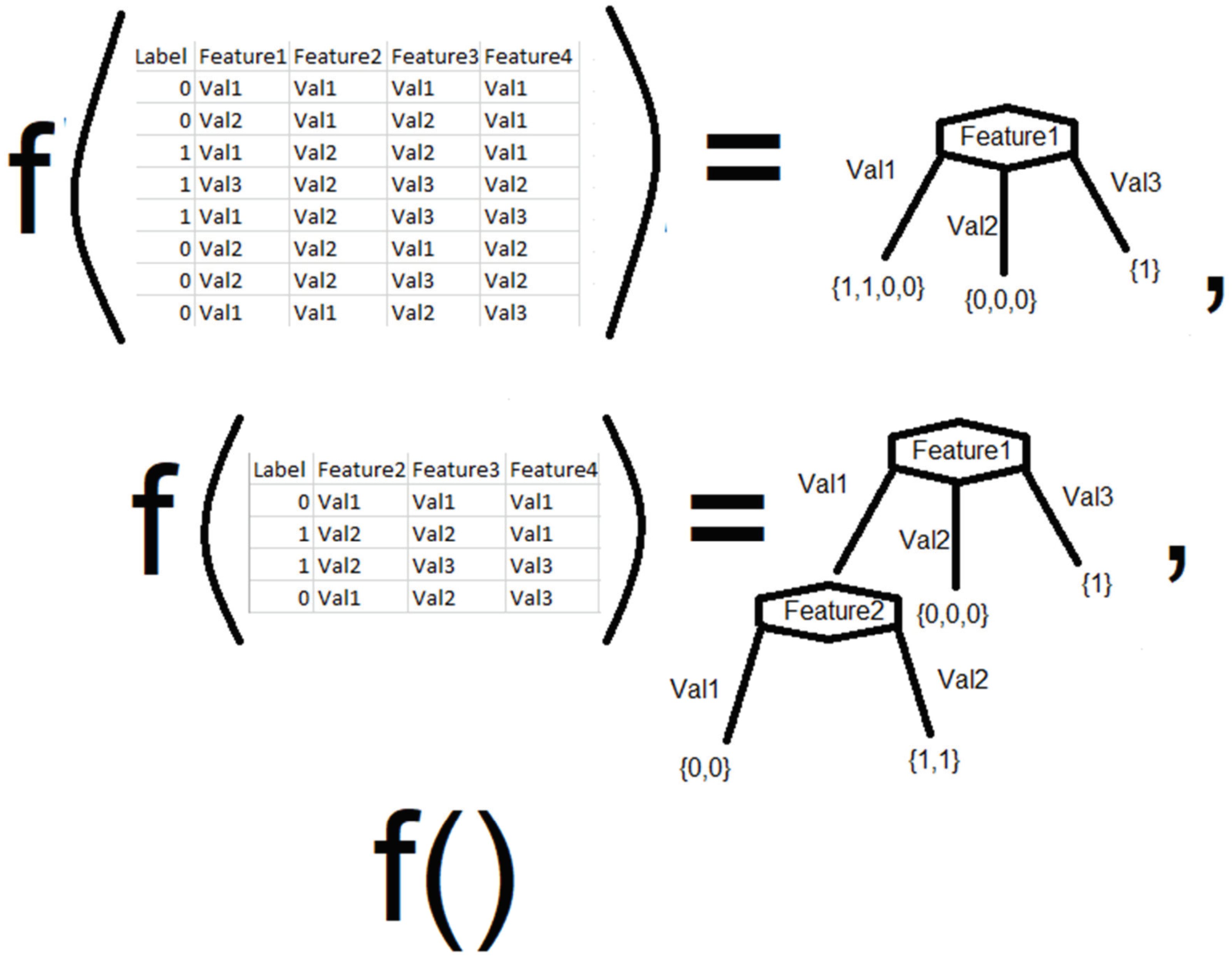
• In the present study, a simple algorithm enhancement to the decision tree algorithm, called the greedy decision tree (GDT), is proposed. The GDT technique involves iteratively constructing a DT, selecting features that give the best results when added to the previously constructed DT. It is shown that the results of this approach are comparable or better than those obtained by Ahuja et al. and Elsayed et al. [1,2].
• Stability analysis of the GDT algorithm is performed to demonstrate its behavior under different conditions while using the aforementioned two SDN-specific datasets.

4. Proposed Approach

This section discusses the proposed approach. First, the motivation behind the proposed approach is presented, which evolves from the discussion in Section 1. This is followed by the DT-based approach adopted in this study.

4.1. Motivation

The proposed algorithm is based on DT, in contrast to the other algorithms mentioned in Section 1. The reasons for this selection are discussed below.

4.1.1. Why Decision Tree?

When creating an ML model, the model’s accuracy is not the only thing of paramount importance. The model needs to be both accurate and interpretable [59], especially when an understanding of the dataset is required. The KNN model is considered to be one of the simplest ML models. However, KNN requires some kind of encoding for categorical variables, as it depends upon the number line for creating classification criterion. This makes KNN unsuitable for data that have features existing on different scales, and in Ahuja et al. [1], KNN does not give the best accuracy.

The logistic regression model also gives bad results even though it is interpretable. SVC and ANNs are black box models [60]. RF is an interpretable model, but Ahuja et al. [1] showed that it did not give the best accuracy. In addition, RF depends on a large number of decision trees. The best model was the one that used SVC in conjunction with RFs, but as discussed above, SVC is a black box, and using such models can be dangerous [61]. Thus, it was concluded that models that perform feature selection and are interpretable should be selected. DTs have both these advantages [62].

4.1.2. Reduction in Computational Complexity

Ahuja et al. [1] proposed the use of t-SNE before applying ML algorithms. t-SNE first develops a probability distribution using the dataset, such that it starts to assign conditional probability to all tuples, thus answering the question of classification in terms of probability. Given a tuple of a particular class, it is necessary to know what the distance around it is, or the neighborhood around it related to the same class. The following formula is used to make this calculation:

$$p_{j|i}={\displaystyle \frac{exp\left(-\frac{\parallel x_i-x_j{\parallel }^2}{2{\sigma }_i^2}\right)}{{\sum }_{k\ne i}exp{\left(-\frac{\parallel x_i-x_k{\parallel }^2}{2{\sigma }_i^2}\right)}^{\prime }}}$$

(1)

In the above formula, $p_{j|i}$ is the probability of point j being selected as the neighbor of point i in the dataset. The reason for taking the exponent of the L2 norm divided by the Gaussian variance is simply to make sure that data points that are distant will have an extremely low probability of being selected. The value of $\sigma$ is found using another variable called perplexity. The value of perplexity is usually taken between 5 and 50, and indicates how many neighbors should be considered between these two values. This value then leads to the selection of the optimum value for $\sigma$ through an algorithm (the explanation is beyond the scope of this paper).

The next step is to obtain a low-dimensional space in which the same distribution with the same number of points exists. For this, we use the t-distribution as it helps avoid the crowding problem, with a single degree of freedom making the above formula into the one below:

$$q_{j|i}={\displaystyle \frac{exp\left(-\parallel y_i-y_j{\parallel }^2\right)}{{\sum }_{k\ne i}exp{\left(-\parallel y_i-y_k{\parallel }^2\right)}^{\prime }}}$$

(2)

Afterwards, the gradient descent algorithm is used to calculate this particular distribution by optimizing the Kullback–Leibler divergence represented by $KL$.

$$C=\sum _{i}KL(P_i\left|\right|Q_i)=\sum _i\sum _j{p}_{j|i}log{\displaystyle \frac{p_{j|i}}{q_{j|i}}}$$

(3)

where C is the cost. In order to minimize C, the correct dimensions need to be selected in the values of y. The derivative of the cost function then becomes as follows:

$${\displaystyle \frac{\partial C}{\partial y_i}}=2\sum _j(p_{j|i}-q_{j|i}+p_{i|j}-q_{i|j})(y_i-y_j)$$

(4)

The literature review explains the implications of using the t-SNE algorithm. It was decided, because of those implications, that applying it would not be of much benefit in the case of the datasets under consideration in this study. Therefore, removing t-SNE removes a whole computation layer used in Ahuja et al. [1], resulting in a more efficient algorithm. The values of $y_i$ and $y_j$ are the new low-dimensional representations of the old points i and j, which were in a high-dimensional space.

4.2. Algorithm Selection

The discussion in Section 4.1 above highlights that the DT algorithm is a strong candidate for the underlying study. However, the question is which variant of DT is the most appropriate choice? The literature has identified several variants of the decision tree. Some well-known algorithms are ID 3 (Iterative Dichotomiser 3) [63], C4.5 (which is a successor of ID3), and CART (classification and regression tree) [64]. Other less-known variants of DT include MARS (multivariate adaptive regression splines) [65] and CHAID (chi-squared automatic interaction detection) [31]. ID3 operates by choosing the best characteristic at each node to partition the data depending on information gain and recursively constructs a tree. The goal is to make the final subsets as homogeneous as possible. By choosing features that offer the greatest reduction in entropy or uncertainty, ID3 iteratively grows the tree. The procedure keeps going until a halting requirement is satisfied, like a minimum subset size or a maximum tree depth.

The core idea is similar in the ID3, C4.5, and CART algorithms. What is required is a decision split that breaks the label data into sets that have the least entropy (a measure of the disorder of a set). Certain steps are common in the three algorithms, which are carried out in the following order:

• Select the attribute with the lowest Gini index/highest information gain/gain ratio.
• Split the initial data into subsets.
• Apply the same technique to the subsets, leaving out the attribute that has already been selected.
• Stop when entropy becomes 0 or no more attributes are left.

A diagrammatic representation of the decision tree construction process is given in Figure 3. The diagram shows that initially, the whole dataset is given as input to the DT construction algorithm. The algorithm selects the best feature from all features and splits the labels of the data accordingly. Then, the DT construction algorithm is applied to the rest of the data, excluding the rows corresponding to the value that gave the best split and excluding that feature. The process is repeated until a tree is obtained with no change in information gain, gain ratio, or Gini index (depending on the tree construction algorithm selected), or when all the features have been used up and there are no more features to be explored. DTs provide the extra advantage of selecting relevant features using either information gain, gain ratio, or Gini index, depending on the algorithm used. All of these feature selection algorithms fall under the category of filter models.

Among ID3, C4.5, and CART, the advantage that CART has is that it is not biased towards multivalued variables like ID3 or towards imbalanced trees like C4.5. The ID3 algorithm does not work on continuous data. Therefore, a discretization layer has to be added to it. As such, the CART algorithm holds a higher potential of showing better performance than ID3 and C4.5, as discussed in detail by Breiman et al. [66]. MARS is generally a good DT algorithm that makes a continuous function, unlike CART, but one drawback is its slower throughput, which can be detrimental in high-speed networks [65]. Additionally, MARS has been shown to be less accurate than CART in some cases [67]. A limitation of CHAID is that the approach performs pre-pruning, which can lead to less accuracy than CART [68,69].

CART uses the Gini index to calculate the relevance of features. This feature selection model creates a binary tree using probabilities of the occurrence of a value of a feature against other features or combinations of other features, using the following formula:

$$GiniIndex\left(f\right)=1-\sum _{i=1}^n{\left(p_i\right|f)}^2$$

(5)

where n corresponds to the number of classes and f is the feature in question belonging to the input. The resultant calculation gives a quantifiable value to judge how much a particular feature is related to the classification.

In this study, the simple CART algorithm is evaluated first. Then, a small modification is done to the CART algorithm where features are added until error starts increasing. In this modified CART algorithm, firstly, a separate DT is made for each feature individually, and the error of each tree is stored. This step is performed more than once so that averages can be considered instead of relying on the results of a single iteration over the features. Then, the average errors are sorted. This also sorts the features in order of the accuracy provided by each feature. Afterwards, features are iteratively added one by one, and a DT is made for each aggregate, stopping when the error of the DT starts to increase. This has the potential to result in a better DT, as now there is a rationality behind including a feature other than its order of appearance in the dataset. The index of features that gives the minimum error has a meaning now. Finally, another algorithm is added that checks the change in accuracy after adding a feature to be considered by the CART algorithm. As a result, features that increase performance or have no effect on it are retained, and features that result in a decrease in performance are dropped following a hill climbing approach.

Hill climbing is a technique that generally starts with an arbitrary solution to a multidimensional problem; then, iteratively, incremental changes are made to the solution, until a better solution is achieved [70]. The problem of feature selection based on model performance is similar to a graph search [71] in that we are trying to find the sequence and relevance of features that lead to the highest accuracy. This poses two options: either go for a slow, optimal, deterministic graph search algorithm, such as A* search; or perform a faster, simpler, but somewhat less optimal greedy search. Eventually, greedy search was chosen because it is faster [72]. The algorithm usually stops after a certain number of iterations, or if the solutions start to become worse than the one already reached, as there is no backtracking [70]. The resulting algorithm, termed greedy decision tree, is used for feature selection using a greedy approach and is illustrated in Algorithm 1.

Algorithm 1 Greedy Decision Tree (F).

1: Input: F (Set of all features)   2: Output: A decision tree constructed using a subset of features   3: S is the set of selected features   4: f is a single feature   5: S ← {} {Initially S is empty}   6: while average of precision, F1-score, accuracy, and false alarm rate on S do not decrease OR $F\ne \left\{\right\}$ do   7:     Construct $\left|F\right|$ decision trees with features in S and each feature in F   8:     Evaluate individual cost of each feature f individually using squared error | f∈F   9:     Select the feature f from F with the minimum cost 10:     $S\leftarrow S\cup \left\{f\right\}$ 11:     Remove f from F 12: end while 13: return S 14: Construct a decision tree with S 15: return the constructed decision tree

5. Performance Measures

The literature has identified several commonly used metrics such as accuracy (A), recall (R), precision (P), specificity (F), false alarm rate (FAR), F1-score, and throughput. Note that accuracy, recall, precision, specificity, and FAR are based on the four primary-level attributes as given below. F1-score is a derived metric based on recall and precision. The four primary-level attributes are as follows [1,73]:

• True positive ($T_P$): legitimate traffic correctly classified as legitimate.
• True negative ($T_N$): illegitimate traffic correctly classified as illegitimate.
• False positive ($F_P$): legitimate traffic incorrectly classified as illegitimate.
• False negative ($F_N$): illegitimate traffic incorrectly classified as legitimate.

Based on the above four attributes, accuracy, which measures the proportion of the total number of correct classifications, is mathematically represented as follows:

$$Accuracy={\displaystyle \frac{T_P+T_N}{T_P+T_N+F_P+F_N}}$$

(6)

Similarly, recall measures the number of correct classifications penalized by the number of missed entries and is represented by the following equation:

$$Recall={\displaystyle \frac{T_P}{T_P+F_N}}$$

(7)

Likewise, precision is a measure of the number of correct classifications penalized by the number of incorrect classifications, as given by the following equation:

$$Precision={\displaystyle \frac{T_P}{T_P+F_P}}$$

(8)

Specificity is defined as the measure of the prediction of the negative class in the dataset and is represented by the following equation:

$$Specificity={\displaystyle \frac{T_N}{T_N+F_P}}$$

(9)

False alarm rate is the measure of inaccurate classification when the model classifies normal traffic as malicious. It is calculated using the following equation:

$$FAR={\displaystyle \frac{F_P}{T_P+F_P}}$$

(10)

The $F1score$ is defined as the measure in which both recall and precision are used. In the case of an unbalanced dataset, we usually calculate the $F1score$. It is defined by the following equation:

$$F1score={\displaystyle \frac{2\times R\times P}{R+P}}$$

(11)

Throughput is also an important measure in analyzing the effectiveness of an ML model [21,29,74,75]. The main argument is that DDoS detection is a time-critical task that is to be performed on high-speed networks. Therefore, high throughput results in low latency [76]. Throughput is measured as follows:

$$Throughput={\displaystyle \frac{Numberofpredictions}{Time}}$$

(12)

6. Results and Discussion

The experiments were carried out on a system with Intel® Core™ i5-5300U CPU @ 2.30 GHz, with two cores and four logical processors with 16 GB RAM, SSD hard disk, and Microsoft Windows 10 Pro for Workstations. Three experiments were carried out. The first experiment evaluated the performance of the CART algorithm as well as the modified CART algorithm. The second experiment compared the proposed GDT algorithm with the techniques proposed by Ahuja et al. [1] and Elsayed et al. [2], as well as some other techniques, while using the two core datasets. The third experiment focused on the stability analysis of the GDT algorithm.

6.1. Comparison of CART and Modified CART Algorithms

The CART decision tree algorithm use all 16 features while incorporating no feature selection other than the one performed by CART. The average performance is measured after splitting the data randomly into training and testing sets in a 80:20 ratio, respectively. Selecting different data partitions results in slight changes in the performance. Therefore, average performance was considered instead of the performance of a single partition of 80:20. The simple CART algorithm was applied, which showed better results compared to the approach proposed by Ahuja et al. [1] The summary of the performance of applying the CART decision tree algorithm is given in

Table 6. Comparison of CART and modified CART algorithms with Ahuja et al. [1].

Algorithm	Accuracy %	Recall %	Specificity %	FAR %	Precision %	F1 Score %	No. of Features
Ahuja	98.8	-	98.18	0.02	98.27	97.65	23
CART	99.990	99.984	99.994	0.009	99.990	99.987	16
Modified CART	99.989	99.985	99.991	0.014	99.986	99.985	10

. The modified CART algorithm was also implemented by iteratively adding features one by one to the training dataset and making a DT in each step. The algorithm stops when the accuracy starts going down. Afterwards, the selected features are used for the prediction of DDoS attack. Table 6 also shows the results achieved by this approach while using Monte Carlo validation. As observed from the table, both CART and modified CART produced results of almost the same quality with respect to different performance measures, but better than that of Ahuja et al. [1] However, the obvious advantage of the modified CART algorithm was with respect to the number of features utilized. In comparison to CART, which used 16 features, the modified CART used 10.1 (rounded off to 10) features on average (based on 10 runs using Monte Carlo), thus making modified CART a better performer.

From the results of the modified CART algorithm, it was observed that even though Ahuja et al. [1] gave a logical explanation of the relevance of the features, not all of them are relevant. There is redundancy in the features as the number of features selected by modified CART is lower. Therefore, it was implied that a feature selection technique, if incorporated before the CART algorithm, might result in a higher accuracy. Accordingly, the simple greedy algorithm in conjunction with CART was tried on the dataset, the details of which follow in the next section.

6.2. Comparison of Proposed Greedy Decision Tree with Other Techniques

This experiment was focused on deciding on a suitable validation approach. For this purpose, the k-fold and Monte Carlo approaches were employed, while using random (unstratified) and stratified sampling. The assessment of the two validation approaches is motivated by past studies, such as the one by Fonseca-Delgado et al. [77]. The problem discussed by Fonseca-Delgado [77] was related to time series forecasting, where the results showed that the Monte Carlo approach produced more stable results. Similarly, Patro [78] compares the two approaches, mentioning that the possible partitions in k-fold are limited by k, whereas the possible partitions are many in Monte Carlo. This implies that models trained using Monte Carlo show repeatable results, which is more desirable in a practical application. However, not much information can be implied about the nature of the data, and how the model works in the case of diverse data, which might occur in exceptional cases. For the latter case, k-fold seems more ideal. Therefore, in this study, both techniques were used. In addition, the work carried out in this experiment was also benchmarked against the techniques presented in the studies by Ahuja et al. [1] and Elsayed et al. [2], as well as many other techniques, namely AdaBoost [79], LogitBoost [79], GentleBoost [79], and RUSBoost [79]. It should be noted that the prior work reported in Ahuja et al. [1] did not mention which validation approach was adopted, whereas Elsayed et al. [2] mentioned using five-fold cross validation.

The next issue was to decide whether to use stratified sampling or random sampling for the training and testing datasets. On the question of whether or not to stratify, a recent study [80] mentions that stratification has advantages over random sampling, but defining strata can be difficult with incomplete knowledge. In the case of the present study, a supervised learning approach is performed, which itself required previously classified data, on the basis of which the classification criteria are to be constructed using an ML model. However, in another study, Elfil and Negida [81] addressed the topic of sampling and specified that stratified sampling is a better approach because it makes in-class differences more apparent. Furthermore, Forman and Scholz [82] mention that stratification lessens experimental variance.

Table 7. Comparison of GDT variants with SVC-RF of Ahuja et al. [1] and other algorithms.

Algorithm	Validation	Sampling	Accuracy %	Recall %	Specificity %	FAR %	Precision %	F1-Score %
GDT	K-Fold	Stratified	99.999	100	99.998	0.00263	99.997	99.999
GDT	K-Fold	Random	99.993	99.989	99.996	0.0052	99.994	99.992
GDT	Monte	Random	99.993	99.995	99.993	0.011	99.980	99.990
	Carlo
AdaBoost	K-Fold	Stratified	97.99	98.13	98.13	2.33	97.66	97.90
LogitBoost	K-Fold	Stratified	98.73	98.80	98.80	1.46	98.53	98.66
GentleBoost	K-Fold	Stratified	99.32	99.32	99.32	0.75	99.24	99.28
RUSBoost	K-Fold	Stratified	88.78	90.77	90.77	11.44	88.55	89.64
SVC-RF (Ahuja)	Not specified	Not specified	98.8	97.91	98.18	0.02	98.27	97.65

shows the results of GDT construction with k-fold and Monte Carlo, with and without stratification, while using the dataset proposed by Ahuja et al. The best results achieved in the study of Ahuja et al. (adopted from [1]) are also reflected in the table.

With regard to the performance measures identified in Section 5 (excluding throughput), the results indicate that with the exception of FAR, the performance with respect to all measures is more or less the same. For FAR, GDT with k-fold and stratified sample produced the minimum value of 0.00263. Table 6 also provides the results produced by the hybrid SVC-RD algorithm of Ahuja et al. [1] Note that Ahuja et al. [1] did not specify what validation or sampling approaches were used. Therefore, the results were adopted as reported in their paper. Based on the comparison of the three variants of GDT with the SVC-RF, AdaBoost, LogitBoost, GentleBoost, and RUSBoost, it can be fairly claimed that all versions of GDT were better than SVC-RF and the other algorithms with respect to the six performance measures.

The GDT algorithms were also compared with the work of Elsayed et al. [2], who employed the RF algorithm with k-fold validation. Their study did not highlight what sampling strategy was adopted. As such, the results from their study were adopted and compared with the GDT variants proposed herein, while using the same dataset as used by Elsayed et al. [2].

Table 8. Comparison of GDT variants with RF of Elsayed et al. [2] and other algorithms.

Algorithm	Validation	Sampling	Accuracy %	Recall %	Specificity %	FAR %	Precision %	F1-Score %
GDT	K-fold	Stratified	99.997	99.995	100	0	100	99.997
GDT	K-fold	Random	99.997	99.995	100	0	100	99.997
GDT	Monte Carlo	Random	99.997	99.995	100	0	100	99.998
AdaBoost	K-fold	Stratified	99.998	99.998	99.998	0.001	99.998	99.998
LogitBoost	K-fold	Stratified	99.996	99.996	99.996	0.003	99.996	99.996
GentleBoost	K-fold	Stratified	99.995	99.995	99.995	0.004	99.995	99.995
RUSBoost	K-fold	Stratified	99.341	99.323	99.301	0.617	99.332	99.341
RF (Elsayed)	K-fold	-	-	99.995	-	-	99.99	99.997

shows the results obtained with different GDT variants, as well as those of Elsayed et al., AdaBoost, LogitBoost, GentleBoost, and RUSBoost. Note that Elsayed et al. [2] used only three performance measures (recall, precision, and F1-score). With regard to these three performance measures, the results found for RF by Elsayed et al. [2] and those for the proposed GDT variants were comparable and of the same quality. Furthermore, the three GDT variants also produced almost the same results, indicating that the different validation and sampling strategies did not have an impact on the performance. In addition, the results produced by the other four algorithms were also comparable with those of GDT.

Table 9. Comparison of average training time and throughput of GDT with other algorithms.

Algorithm	Validation	Sampling	Average Training Time		Throughput (Predictions/Sec)
			Ahuja	Elsayed	Ahuja	Elsayed
GDT	K-fold	Stratified	8.0	7.6	2,658,798	5,723,790
GDT	K-fold	Random	8.0	7.6	2,509,367	5,714,573
GDT	Monte Carlo	Random	8.0	7.6	2,753,333	5,718,750
AdaBoost	K-fold	Stratified	10.1	9.7	147,618	252,850
LogitBoost	K-fold	Stratified	11.5	8.5	164,636	283,262
GentleBoost	K-fold	Stratified	8.9	7.9	193,814	294,309
RUSBoost	K-fold	Stratified	13.1	16.4	195,295	269,154
SVC-RF (Ahuja)	-	-	-	-	-	-
RF (Elsayed)	K-fold	-	-	42.5	-	-

reflects the average training time and throughput of the proposed GDT. Note that Ahuja et al. [1] and Elsayed et al. [2] did not share the hyperparameter values they used in their respective studies. Therefore, it was not possible to reproduce their results, as both of their algorithms depend upon hyperparameters. It is clearly visible from the table that with respect to the average training time (in seconds), GDT results in much lower training times than all other algorithms for both datasets. The same level of performance is observed for throughput, where GDT has far higher throughput than the other algorithms.

It should be noted that although better results were obtained using the proposed approach, these results only represent high performance in the simulated dataset. It is not necessary that this better performance would be reflected in real-world scenarios, as reported by similar studies [53,54].

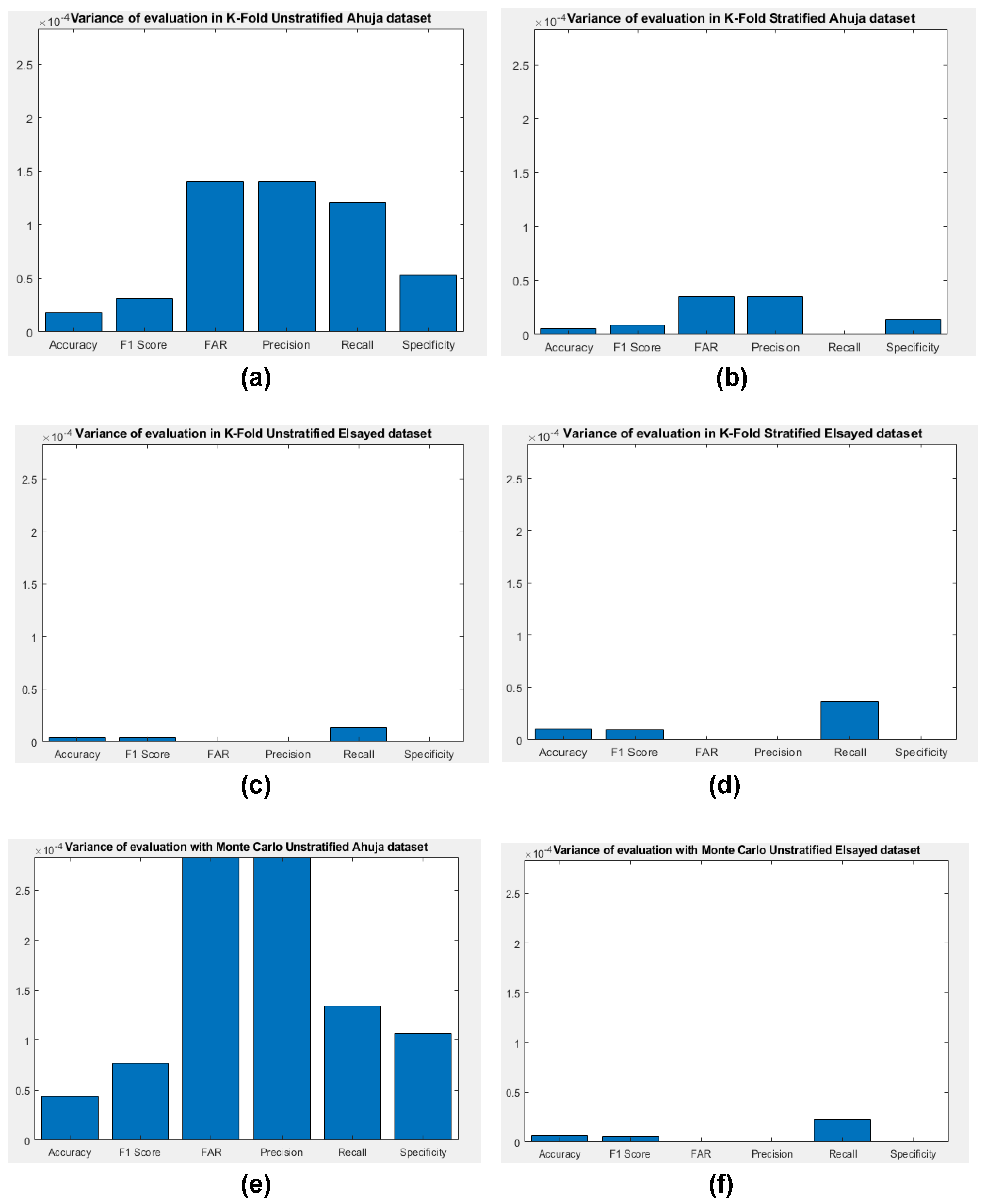
6.3. Stability Analysis of the Greedy Decision Tree Algorithm

The results in Section 6.2 highlight the superior performance of GDT variants compared to other recent algorithms. However, a further in-depth analysis is required to evaluate the stability of the GDT approach. Last et al. [83] propose that overall misclassification rate is a very basic measure of the stability of decision trees. They further point towards the direction of measuring variations in the prediction to measure the stability of decision trees. In accordance with this, the plots in Figure 4 depict variance for the three GDT variants with respect to the different evaluation metrics.

As far as the variance in evaluation parameters is concerned, the GDT algorithm results in an extremely lower variance, as can be verified from the bar graphs in Figure 4. The bar graphs show that in case of the dataset in Ahuja et al. [1], k-fold cross validation with stratification (Figure 4b) gives the lowest variance, and k-fold without stratification (Figure 4a) gives a higher variance than k-fold stratified data, while Monte Carlo gives the highest variance (Figure 4e) for all performance measures. In the case of the dataset of Elsayed et al. [2], the lowest variance is achieved when using k-fold without stratification (Figure 4c), a higher variance is obtained with Monte Carlo (as shown in Figure 4f), and the highest variance is shown when using k-fold with stratification (Figure 4d).

The stability of the GDT algorithm was also evaluated in terms of the variance in the number of features selected and the tree size. Such a stability measure for decision trees was advocated by Jaccobucci [84], who identified how class agreement on different folds and decision tree structures can help measure the stability of decision trees. Keeping this under consideration,

Table 10. Analysis of variances in features and tree size for the two datasets with GDT.

Dataset	Sampling	Validation	Feature Variance	Tree Size Variance
Ahuja	Stratified	K-fold	0.2	57.2
Ahuja	Not stratified	K-fold	0.7	215.2
Ahuja	Not stratified	Monte Carlo	0.3447	685.47
Elsayed	Stratified	K-fold	0.2	156
Elsayed	Not stratified	K-fold	0.3	270.8
Elsayed	Not stratified	Monte Carlo	0.213	152.78

summarizes the results of experiments to measure the variance in tree structure and features used in different combinations of validation testing. It is observed that in the case of the dataset of Ahuja et al. [1], the variance in the number of features selected is quite low for all sampling and validation types. Similar observations are made for the dataset of Elsayed et al. [2] In terms of the tree size: the variance in tree structure is the lowest for k-fold stratified, with a value of 57.2. In general, k-fold gives better results than Monte Carlo (which shows a very high variance of 685.47). In the case of Elsayed et al. [2], a more stable tree structure is achieved with Monte Carlo.

The implications of k-fold cross-validation providing a more stable model can point to multiple attributes of the dataset. It could mean that the features in the dataset are more robust, as was claimed by Ahuja et al. [1] It could also point to the homogeneity of the dataset, which is a good quality in terms of there being fewer outliers in the dataset. It could also mean that the dataset is highly representative. Similarly, a more stable structure with Monte Carlo could point to a lack of the abovementioned features in the dataset of Elsayed et al. [2] A conclusive statement would require an in-depth data analysis of both datasets, which can be future work for another study.

The slightly higher accuracy in the case of stratified k-fold cross-validation in the dataset of Ahuja et al. [1] might be due to a minor imbalance, or if the imbalance is there, in the data patterns for classification [85]. Therefore, even though the datasets are balanced, it is highly probable that the dataset in Elsayed et al. [2] has more information uniformly spread out. However, this is a speculation. The slightly higher accuracy could also be due to the slightly larger size of the dataset in Elsayed et al. [2] since dataset size also has a strong link with accuracy [86]. What is required is a detailed study of the statistical properties of this dataset.

The effects of feature values are discussed in a recent study [87], where it shows that feature drift, i.e., the change in environmental feature values over time, can cause the model to malfunction. This can significantly change the training outcome if the test set has features far away from the features in the training set. Furthermore, it has been documented by Ahmadi et al. [88] that datasets that have high variance or noise perform better with stratified k-fold cross-validation, as it makes sure that the model generalizes well with different subsets of the dataset.

7. Limitations of the Proposed Method

Although the proposed GDT has shown performance improvements, the approach also has certain limitations, as described below.

High variance estimators: Decision trees are very prone to data variations [89]. Nevertheless, our experiments show that even in the case of data variations, a good overall accuracy was achieved. However, our high accuracy might not be representative of real-world data. More work needs to be done in this direction.

Difficulty in nonlinear decision boundaries: Due to stepwise decisions, it is difficult to grasp nonlinear decision boundaries [90].

High computation time: The iterative approach of adding features on the basis of overall model accuracy is very helpful in achieving high accuracy and FAR. However, it has a higher computational cost than conventional DTs and RF classifiers. The tradeoff is that it is more interpretable and more accurate [57].

8. Conclusions and Future Directions

Software-defined networks are prone to DDoS attacks. A promising approach to address this issue is to employ classification algorithms that are capable of segregating genuine and bogus requests. Machine learning algorithms have been extensively utilized to study the phenomenon using different datasets. One of the well-established machine learning approaches is the decision tree, which has several strong features compared to other machine learning algorithms. This study evaluated several decision tree algorithms while using two recent SDN-specific datasets proposed by Ahuja et al. [1] and Elsayed et al. [2]. In comparison with the best performer of Ahuja et al. [1] (i.e., SVC-RF classifier) and Elsayed et al. [2] (random forest), as well as the AdaBoost, LogitBoost, GentleBoost, and RUSBoost algorithms, the GDT approach demonstrated better or comparable performance with respect to the standard performance measures. The GDT also showed low average training times and high throughput. Furthermore, it was verified that the proposed GDT approach creates decision trees that have low variance when it comes to predictability.

Overall, it can be concluded that the GDT approach presented in this study gives better results with two different datasets, using a simple ML model that does not depend upon hyperparameter tuning. Although the accuracy achieved is not too significant, the impact of this slight increase in accuracy is still worth noticing because according to a recent report [91], the cost incurred due to DDoS attacks is usually GBP 325,000 per attack. Thus, in the case of Ahuja et al. [1], the GDT results in an increase of 1.2% in accuracy, which actually translates to the detection of 1252 more attacks. In economic terms, this means speculatively saving a lot of money, but only if the simulated datasets in Ahuja et al. [1] are representative of real-world attack scenarios. These results start to appear even better when one incorporates data shared by Cisco that predict a 1.5 million yearly increase in DDoS attacks [92]. In the case of Elsayed et al. [2], it can be said that the computational cost of running a random forest is far more excessive than that of a simple decision tree. Thus, applying GDT on both datasets shows that the tree is somewhat generalizable in terms of its prediction power. One more point that needs to be mentioned is that GDT is capable of achieving the same or better accuracy while being a simpler and computationally cheaper technique, an idea which goes against Spearman’s law of diminishing returns. This law states that, if the amount of input of a production process continuously increases and all of the other production factors stay constant, the rate of growth of the output will eventually decrease. This means that returns are diminished at a certain level as a consequence of expanding the volume of input [93], as has been shown previously [94].

The work can be expanded in several dimensions. Detailed study can be performed in the direction of feature selection using better techniques as this can lead to more stable decision trees. Furthermore, analysis of the data should be performed so as to observe whether or not the datasets themselves have some intrinsic limitations. This may lead to the development of more robust datasets. The use of deep learning techniques can also be explored for the underlying problem.

References

1. Ahuja, N.; Singal, G.; Mukhopadhyay, D.; Kumar, N. Automated DDOS attack detection in software defined networking. J. Netw. Comput. Appl. 2021, 187, 103108. [Google Scholar] [CrossRef]
2. Elsayed, M.S.; Le-Khac, N.A.; Jurcut, A.D. InSDN: A novel SDN intrusion dataset. IEEE Access 2020, 8, 165263–165284. [Google Scholar] [CrossRef]
3. Javaid, S.; Afzal, H.; Babar, M.; Arif, F.; Tan, Z.; Jan, M.A. ARCA-IoT: An attack-resilient cloud-assisted IoT system. IEEE Access 2019, 7, 19616–19630. [Google Scholar] [CrossRef]
4. Babar, M.; Tariq, M.U.; Jan, M.A. Secure and resilient demand side management engine using machine learning for IoT-enabled smart grid. Sustain. Cities Soc. 2020, 62, 102370. [Google Scholar] [CrossRef]
5. Eliyan, L.F.; Di Pietro, R. DoS and DDoS attacks in Software Defined Networks: A survey of existing solutions and research challenges. Future Gener. Comput. Syst. 2021, 122, 149–171. [Google Scholar] [CrossRef]
6. Nicholson, P. AWS hit by Largest Reported DDoS Attack of 2.3 Tbps. 2023. Available online: https://www.a10networks.com/blog/aws-hit-by-largest-reported-ddos-attack-of-2-3-tbps/ (accessed on 3 October 2023).
7. Bhaya, W.; Manaa, M.E. Review clustering mechanisms of distributed denial of service attacks. J. Comput. Sci. 2014, 10, 2037. [Google Scholar] [CrossRef]
8. Rehman, A.; Haseeb, K.; Alam, T.; Alamri, F.S.; Saba, T.; Song, H. Intelligent secured traffic optimization model for urban sensing applications with Software Defined Network. IEEE Sens. J. 2024, 24, 5654–5661. [Google Scholar]
9. Nadeem, M.W.; Goh, H.G.; Ponnusamy, V.; Aun, Y. DDoS Detection in SDN using Machine Learning Techniques. Comput. Mater. Contin. 2021, 71, 771–789. [Google Scholar]
10. Palmieri, F. Network anomaly detection based on logistic regression of nonlinear chaotic invariants. J. Netw. Comput. Appl. 2019, 148, 102460. [Google Scholar]
11. Santos, R.; Souza, D.; Santo, W.; Ribeiro, A.; Moreno, E. Machine learning algorithms to detect DDoS attacks in SDN. Concurr. Comput. Pract. Exp. 2019, 32, e5402. [Google Scholar] [CrossRef]
12. Niyaz, Q.; Sun, W.; Javaid, A. A deep learning based DDoS detection system in software-defined networking (SDN). arXiv 2016, arXiv:1611.07400. [Google Scholar]
13. da Silva, A.S.; Wickboldt, J.A.; Granville, L.Z.; Schaeffer-Filho, A. ATLANTIC: A framework for anomaly traffic detection, classification, and mitigation in SDN. In Proceedings of the NOMS 2016-2016 IEEE/IFIP Network Operations and Management Symposium, Istanbul, Turkey, 25–29 April 2016; pp. 27–35. [Google Scholar]
14. Bahashwan, A.A.; Anbar, M.; Manickam, S.; Al-Amiedy, T.A.; Aladaileh, M.A.; Hasbullah, I.H. A Systematic Literature Review on Machine Learning and Deep Learning Approaches for Detecting DDoS Attacks in Software-Defined Networking. Sensors 2023, 23, 4441. [Google Scholar] [CrossRef] [PubMed]
15. Karan, B.; Narayan, D.; Hiremath, P. Detection of DDoS attacks in software defined networks. In Proceedings of the 2018 3rd International Conference on Computational Systems and Information Technology for Sustainable Solutions (CSITSS), Bengaluru, India, 20–22 December 2018; pp. 265–270. [Google Scholar]
16. Yang, L.; Zhao, H. DDoS attack identification and defense using SDN based on machine learning method. In Proceedings of the 2018 15th International Symposium on Pervasive Systems, Algorithms and Networks (I-SPAN), Yichang, China, 16–18 October 2018; pp. 174–178. [Google Scholar]
17. Sudar, K.M.; Beulah, M.; Deepalakshmi, P.; Nagaraj, P.; Chinnasamy, P. Detection of Distributed Denial of Service Attacks in SDN using Machine learning techniques. In Proceedings of the 2021 International Conference on Computer Communication and Informatics (ICCCI), Coimbatore, India, 27–29 January 2021; pp. 1–5. [Google Scholar]
18. Kavitha, M.; Suganthy, M.; Biswas, A.; Srinivsan, R.; Kavitha, R.; Rathesh, A. Machine Learning Techniques for Detecting DDoS Attacks in SDN. In Proceedings of the 2022 International Conference on Automation, Computing and Renewable Systems (ICACRS), Pudukkottai, India, 13–15 December 2022; pp. 634–638. [Google Scholar]
19. Wang, S.; Balarezo, J.F.; Chavez, K.G.; Al-Hourani, A.; Kandeepan, S.; Asghar, M.R.; Russello, G. Detecting flooding DDoS attacks in software defined networks using supervised learning techniques. Eng. Sci. Technol. Int. J. 2022, 35, 101176. [Google Scholar]
20. Revathi, M.; Ramalingam, V.; Amutha, B. A machine learning based detection and mitigation of the DDOS attack by using SDN controller framework. Wirel. Pers. Commun. 2022, 127, 2417–2441. [Google Scholar] [CrossRef]
21. Gebremeskel, T.G.; Gemeda, K.A.; Krishna, T.G.; Ramulu, P.J. DDoS Attack Detection and Classification Using Hybrid Model for Multicontroller SDN. Wirel. Commun. Mob. Comput. 2023, 9965945. [Google Scholar] [CrossRef]
22. Elubeyd, H.; Yiltas-Kaplan, D. Hybrid Deep Learning Approach for Automatic DoS/DDoS Attacks Detection in Software-Defined Networks. Appl. Sci. 2023, 13, 3828. [Google Scholar]
23. Hassan, A.I.; El Reheem, E.A.; Guirguis, S.K. An entropy and machine learning based approach for DDoS attacks detection in software defined networks. Sci. Rep. 2024, 14, 18159. [Google Scholar]
24. Luong, T.K.; Tran, T.D.; Le, G.T. DDoS attack detection and defense in SDN based on machine learning. In Proceedings of the 2020 7th NAFOSTED Conference on Information and Computer Science (NICS), Ho Chi Minh City, Vietnam, 26–27 November 2020; pp. 31–35. [Google Scholar]
25. Alamri, H.A.; Thayananthan, V. Analysis of machine learning for securing software-defined networking. Procedia Comput. Sci. 2021, 194, 229–236. [Google Scholar] [CrossRef]
26. Karki, D.; Dawadi, B.R. Machine Learning based DDoS Detection System in Software-Defined Networking. In Proceedings of the 11th IOE Graduate Conference, Pokhara, Nepal, 9–10 March 2022; pp. 228–246. [Google Scholar]
27. Dheyab, S.A.; Abdulameer, S.M.; Mostafa, S. Efficient Machine Learning Model for DDoS Detection System Based on Dimensionality Reduction. Acta Inform. Pragensia 2022, 11, 348–360. [Google Scholar]
28. Sanmorino, A.; Marnisah, L.; Di Kesuma, H. Detection of DDoS Attacks using Fine-Tuned Multi-Layer Perceptron Models. Eng. Technol. Appl. Sci. Res. 2024, 14, 16444–16449. [Google Scholar] [CrossRef]
29. Mehmood, S.; Amin, R.; Mustafa, J.; Hussain, M.; Alsubaei, F.S.; Zakaria, M.D. Distributed Denial of Services (DDoS) attack detection in SDN using Optimizer-equipped CNN-MLP. PLoS ONE 2025, 20, e0312425. [Google Scholar] [CrossRef] [PubMed]
30. Rahman, O.; Quraishi, M.A.G.; Lung, C.H. DDoS attacks detection and mitigation in SDN using machine learning. In Proceedings of the 2019 IEEE World Congress on Services (SERVICES), Milan, Italy, 8–13 July 2019; Volume 2642, pp. 184–189. [Google Scholar]
31. Almadhor, A.; Altalbe, A.; Bouazzi, I.; Hejaili, A.A.; Kryvinska, N. Strengthening network DDOS attack detection in heterogeneous IoT environment with federated XAI learning approach. Sci. Rep. 2024, 14, 24322. [Google Scholar] [CrossRef]
32. Kyaw, A.T.; Oo, M.Z.; Khin, C.S. Machine-learning based DDOS attack classifier in software defined network. In Proceedings of the 2020 17th International Conference on Electrical Engineering/Electronics, Computer, Telecommunications and Information Technology (ECTI-CON), Phuket, Thailand, 24–27 June 2020; pp. 431–434. [Google Scholar]
33. Firdaus, D.; Munadi, R.; Purwanto, Y. Ddos attack detection in software defined network using ensemble k-means++ and random forest. In Proceedings of the 2020 3rd International Seminar on Research of Information Technology and Intelligent Systems (ISRITI), Yogyakarta, Indonesia, 10–11 December 2020; pp. 164–169. [Google Scholar]
34. Nugraha, B.; Murthy, R.N. Deep learning-based slow DDoS attack detection in SDN-based networks. In Proceedings of the 2020 IEEE Conference on Network Function Virtualization and Software Defined Networks (NFV-SDN), Leganes, Spain, 10–12 November 2020; pp. 51–56. [Google Scholar]
35. Alshra’a, A.S.; Farhat, A.; Seitz, J. Deep learning algorithms for detecting denial of service attacks in software-defined networks. Procedia Comput. Sci. 2021, 191, 254–263. [Google Scholar] [CrossRef]
36. Altamemi, A.J.; Abdulhassan, A.; Obeis, N.T. DDoS attack detection in software defined networking controller using machine learning techniques. Bull. Electr. Eng. Inform. 2022, 11, 2836–2844. [Google Scholar] [CrossRef]
37. Karthika, P.; Arockiasamy, K. Simulation of SDN in mininet and detection of DDoS attack using machine learning. Bull. Electr. Eng. Inform. 2023, 12, 1797–1805. [Google Scholar] [CrossRef]
38. Kannan, C.; Muthusamy, R.; Srinivasan1, V.; Chidambaram, V.; Karunakaran, K. Machine learning based detection of DDoS attacks in software defined network. Indones. J. Electr. Eng. Comput. Sci. 2023, 32, 1503–1511. [Google Scholar] [CrossRef]
39. Hassan, H.A.; Hemdan, E.E.D.; El-Shafai, W.; Shokair, M.; Abd El-Samie, F.E. Detection of attacks on software defined networks using machine learning techniques and imbalanced data handling methods. Secur. Priv. 2024, 7, e350. [Google Scholar] [CrossRef]
40. Haq, I.; Khan, S.A.; Mohammad, N.; Zaman, A. Optimizing Distributed Denial of Service (DDoS) Attack Detection Techniques on Software Defined Network (SDN) Using Feature Selection. In Proceedings of the 2024 4th International Conference on Innovations in Computer Science (ICONICS), Karachi, Pakistan, 13–14 November 2024; pp. 1–7. [Google Scholar]
41. Potdar, K.; Pardawala, T.S.; Pai, C.D. A comparative study of categorical variable encoding techniques for neural network classifiers. Int. J. Comput. Appl. 2017, 175, 7–9. [Google Scholar] [CrossRef]
42. Hancock, J.T.; Khoshgoftaar, T.M. Survey on categorical data for neural networks. J. Big Data 2020, 7, 1–41. [Google Scholar] [CrossRef]
43. Duan, J. Financial system modeling using deep neural networks (DNNs) for effective risk assessment and prediction. J. Frankl. Inst. 2019, 356, 4716–4731. [Google Scholar] [CrossRef]
44. Trunk, G.V. A problem of dimensionality: A simple example. IEEE Trans. Pattern Anal. Mach. Intell. 1979, PAMI-1, 306–307. [Google Scholar]
45. Wheeler, A. PCA Does Not Make Sense After One Hot Encoding. 2021. Available online: https://andrewpwheeler.com/2021/06/22/pca-does-not-make-sense-after-one-hot-encoding/ (accessed on 12 December 2023).
46. Ghosh, A.M.; Grolinger, K. Deep learning: Edge-cloud data analytics for iot. In Proceedings of the 2019 IEEE Canadian Conference of Electrical and Computer Engineering (CCECE), Edmonton, AB, Canada, 5–8 May 2019; pp. 1–7. [Google Scholar]
47. Linting, M.; Meulman, J.J.; Groenen, P.J.; van der Koojj, A.J. Nonlinear principal components analysis: Introduction and application. Psychol. Methods 2007, 12, 336. [Google Scholar] [PubMed]
48. Van der Maaten, L.; Hinton, G. Visualizing data using t-SNE. J. Mach. Learn. Res. 2008, 9, 2579–2605. [Google Scholar]
49. Xu, X.; Xie, Z.; Yang, Z.; Li, D.; Xu, X. A t-SNE based classification approach to compositional microbiome data. Front. Genet. 2020, 11, 620143. [Google Scholar]
50. Vidyala, R. What, Why and How of t-SNE. 2020. Available online: https://medium.com/data-science/what-why-and-how-of-t-sne-1f78d13e224d#:~:text=t%2DSNE%20plots%20are%20highly,parameter%20for%20all%20the%20runs (accessed on 11 November 2023).
51. Shah, R.; Silwal, S. Using dimensionality reduction to optimize t-sne. arXiv 2019, arXiv:1912.01098. [Google Scholar]
52. Waagen, D.; Hulsey, D.; Godwin, J.; Gray, D.; Barton, J.; Farmer, B. t-SNE or not t-SNE, that is the question. In Proceedings of the Automatic Target Recognition XXXI, SPIE, Online, 12–16 April 2021; Volume 11729, pp. 62–71. [Google Scholar]
53. Bahashwan, A.A.; Anbar, M.; Manickam, S.; Issa, G.; Aladaileh, M.A.; Alabsi, B.A.; Rihan, S.D.A. HLD-DDoSDN: High and low-rates dataset-based DDoS attacks against SDN. PLoS ONE 2024, 19, e0297548. [Google Scholar]
54. Negera, W.G.; Schwenker, F.; Debelee, T.G.; Melaku, H.M.; Feyisa, D.W. Lightweight model for botnet attack detection in software defined network-orchestrated IoT. Appl. Sci. 2023, 13, 4699. [Google Scholar] [CrossRef]
55. Abtahi, S.M.; Rahmani, H.; Allahgholi, M.; Alizadeh Fard, S. ENIXMA: ENsemble of EXplainable Methods for detecting network Attack. Comput. Knowl. Eng. 2024, 7, 1–8. [Google Scholar]
56. Navia-Vázquez, A.; Parrado-Hernández, E. Support vector machine interpretation. Neurocomputing 2006, 69, 1754–1759. [Google Scholar]
57. Brüggenjürgen, S.; Schaaf, N.; Kerschke, P.; Huber, M.F. Mixture of Decision Trees for Interpretable Machine Learning. In Proceedings of the 2022 21st IEEE International Conference on Machine Learning and Applications (ICMLA), Nassau, Bahamas, 12–14 December 2022; pp. 1175–1182. [Google Scholar]
58. Zhou, Q.; Li, R.; Xu, L.; Nallanathan, A.; Yang, J.; Fu, A. Towards Interpretable Machine-Learning-Based DDoS Detection. SN Comput. Sci. 2023, 5, 115. [Google Scholar]
59. Pandey, P. Interpretable or Accurate? Why Not Both? 2021. Available online: https://towardsdatascience.com/interpretable-or-accurate-why-not-both-4d9c73512192 (accessed on 16 February 2024).
60. Dinov, I.D.; Dinov, I.D. Black box machine-learning methods: Neural networks and support vector machines. In Data Science and Predictive Analytics: Biomedical and Health Applications using R; Springer: Cham, Switzerland, 2018; pp. 383–422. [Google Scholar]
61. Siklar, M. Why Building Black-Box Models Can Be Dangerous. 2021. Available online: https://towardsdatascience.com/why-building-black-box-models-can-be-dangerous-6f885b252818 (accessed on 16 February 2024).
62. Molnar, C. Interpretable Machine Learning. 2020. Available online: https://christophm.github.io/interpretable-ml-book/ (accessed on 25 January 2025).
63. Anonymous. 2024. Available online: https://www.geeksforgeeks.org/iterative-dichotomiser-3-id3-algorithm-from-scratch/ (accessed on 27 October 2024).
64. Abdullah, A.S.; Selvakumar, S.; Karthikeyan, P.; Venkatesh, M. Comparing the efficacy of decision tree and its variants using medical data. Indian J. Sci. Technol. 2017, 10, 1–8. [Google Scholar]
65. MARS, vs. CART Regression Predictive Power. Available online: https://stats.stackexchange.com/questions/584597/mars-vs-cart-regression-predictive-power?newreg=089b481e966f41f1a224a90d681f7c09 (accessed on 8 March 2025).
66. Breiman, L. Classification and Regression Trees; Routledge: Abingdon, UK, 2017. [Google Scholar]
67. Tırınk, C.; Önder, H.; Francois, D.; Marcon, D.; Şen, U.; Shaikenova, K.; Omarova, K.; Tyasi, T.L. Comparison of the data mining and machine learning algorithms for predicting the final body weight for Romane sheep breed. PLoS ONE 2023, 18, e0289348. [Google Scholar]
68. Rashid, R. Digital Analytics Decision Trees; CHAID vs CART. 2017. Available online: https://www.linkedin.com/pulse/digital-analytics-decision-trees-chaid-vs-cart-raymond-rashid/ (accessed on 8 March 2025).
69. Shmueli, G. Classification Trees: CART vs. CHAID. 2007. Available online: https://www.bzst.com/2006/10/classification-trees-cart-vs-chaid.html (accessed on 8 March 2025).
70. González, A.; Pérez, R. An experimental study about the search mechanism in the SLAVE learning algorithm: Hill-climbing methods versus genetic algorithms. Inf. Sci. 2001, 136, 159–174. [Google Scholar]
71. Giarelis, N.; Kanakaris, N.; Karacapilidis, N. An innovative graph-based approach to advance feature selection from multiple textual documents. In Proceedings of the IFIP international Conference on Artificial Intelligence Applications and Innovations, Halkidiki, Greece, 5–7 June 2020; pp. 96–106. [Google Scholar]
72. Kumar, R.R.; Tarang, G.R.; Adipudi, K.K.; Parvathaneni, V.; Steven, G. Performance Comparison of A* Search Algorithm and Hill-Climb Search Algorithm: A Case Study. In Multifaceted approaches for Data Acquisition, Processing & Communication; CRC Press: Boca Raton, FL, USA, 2024; pp. 185–194. [Google Scholar]
73. Khan, S.A.; Iqbal, K.; Mohammad, N.; Akbar, R.; Ali, S.S.A.; Siddiqui, A.A. A Novel Fuzzy-Logic-Based Multi-Criteria Metric for Performance Evaluation of Spam Email Detection Algorithms. Appl. Sci. 2022, 12, 7043. [Google Scholar] [CrossRef]
74. Haseeb-Ur-Rehman, R.M.A.; Aman, A.H.M.; Hasan, M.K.; Ariffin, K.A.Z.; Namoun, A.; Tufail, A.; Kim, K.H. High-speed network ddos attack detection: A survey. Sensors 2023, 23, 6850. [Google Scholar] [CrossRef]
75. Adedeji, K.B.; Abu-Mahfouz, A.M.; Kurien, A.M. DDoS attack and detection methods in internet-enabled networks: Concept, research perspectives, and challenges. J. Sens. Actuator Netw. 2023, 12, 51. [Google Scholar] [CrossRef]
76. Lapolli, Â.C.; Marques, J.A.; Gaspary, L.P. Offloading real-time DDoS attack detection to programmable data planes. In Proceedings of the 2019 IFIP/IEEE Symposium on Integrated Network and Service Management (IM), Arlington, VA, USA, 8–12 April 2019; pp. 19–27. [Google Scholar]
77. Fonseca-Delgado, R.; Gomez-Gil, P. An assessment of ten-fold and Monte Carlo cross validations for time series forecasting. In Proceedings of the 2013 10th International Conference on Electrical Engineering, Computing Science and Automatic Control (CCE), Mexico City, Mexico, 30 September–4 October 2013; pp. 215–220. [Google Scholar]
78. Patro, R. Cross-Validation: K Fold vs. Monte Carlo. 2021. Available online: https://towardsdatascience.com/cross-validation-k-fold-vs-monte-carlo-e54df2fc179b (accessed on 11 November 2023).
79. Ensemble Algorithms. 2024. Available online: https://www.mathworks.com/help/stats/ensemble-algorithms.html (accessed on 7 March 2025).
80. How Do You Choose Between Simple Random and Stratified Sampling? Available online: https://www.linkedin.com/advice/3/how-do-you-choose-between-simple-random-stratified-sampling (accessed on 13 December 2023).
81. Elfil, M.; Negida, A. Sampling methods in clinical research; an educational review. Emergency 2017, 5, e52. [Google Scholar]
82. Forman, G.; Scholz, M. Apples-to-apples in cross-validation studies: Pitfalls in classifier performance measurement. ACM SIGKDD Explor. Newsl. 2010, 12, 49–57. [Google Scholar]
83. Last, M.; Maimon, O.; Minkov, E. Improving stability of decision trees. Int. J. Pattern Recognit. Artif. Intell. 2002, 16, 145–159. [Google Scholar]
84. Jacobucci, R. Decision Tree Stability and Its Effect on Interpretation. Ph.D. Thesis, University of Notre Dame, Notre Dame, IN, USA, 2018. [Google Scholar]
85. Szeghalmy, S.; Fazekas, A. A comparative study of the use of stratified cross-validation and distribution-balanced stratified cross-validation in imbalanced learning. Sensors 2023, 23, 2333. [Google Scholar] [CrossRef]
86. Impact of Dataset Size on Classification Performance. Available online: https://dspace.mit.edu/bitstream/handle/1721.1/131330/applsci-11-00796.pdf?sequence=1 (accessed on 7 March 2025).
87. Kusumura, Y. Maintain Model Robustness: Strategies to Combat Feature Drift in Machine Learning. 2023. Available online: https://dotdata.com/blog/maintain-model-robustness-strategies-to-combat-feature-drift-in-machine-learning/ (accessed on 7 March 2025).
88. Ahmadi, A.; Sharif, S.S.; Banad, Y.M. A Comparative Study of Sampling Methods with Cross-Validation in the FedHome Framework. IEEE Trans. Parallel Distrib. Syst. 2025, 36, 570–579. [Google Scholar] [CrossRef]
89. Decision Trees. Available online: https://www.ibm.com/think/topics/decision-trees (accessed on 7 March 2025).
90. 8 Key Advantages and Disadvantages of Decision Trees. Available online: https://insidelearningmachines.com/advantages_and_disadvantages_of_decision_trees/ (accessed on 7 March 2025).
91. Williams, S. Global Surge in DDoS Attacks Causes Dire Financial Consequences. 2024. Available online: https://securitybrief.in/story/global-surge-in-ddos-attacks-causes-dire-financial-consequences (accessed on 14 March 2024).
92. Smith, G. DDoS Statistics: How Large a Threat Are DDoS Attacks? 2024. Available online: https://www.stationx.net/ddos-statistics/ (accessed on 14 March 2024).
93. Blum, D.; Holling, H. Spearman’s law of diminishing returns. A meta-analysis. Intelligence 2017, 65, 60–66. [Google Scholar] [CrossRef]
94. Hernández-Orallo, J. Is Spearman’s law of diminishing returns (SLODR) meaningful for artificial agents? In Proceedings of the ECAI —22nd European Conference on Artificial Intelligence, The Hague, The Netherlands, 29 August–2 September 2016; pp. 471–479. [Google Scholar]
Figure 1. Architecture of a software-defined network.
Futureinternet 17 00136 g001
Figure 2. DDoS attack architecture in SDN [7].
Futureinternet 17 00136 g002
Figure 3. Example of decision tree construction process.
Futureinternet 17 00136 g003
Figure 4. Variance in performance measures for the two datasets using GDT.
Futureinternet 17 00136 g004