Top-K Feature Selection for IoT Intrusion Detection: Contributions of XGBoost, LightGBM, and Random Forest

Abstract

The rapid growth of the Internet of Things (IoT) has created vast networks of interconnected devices that are increasingly exposed to cyberattacks. Ensuring the security of such distributed systems requires efficient and adaptive intrusion detection mechanisms. However, conventional methods face limitations in processing large and complex feature spaces. To address this issue, this study proposes an optimized intrusion detection approach based on Top-K feature selection combined with ensemble learning models, evaluated on the CICIoMT2024 dataset. Three algorithms, XGBoost, LightGBM, and Random Forest, were trained and tested on IoT datasets using three feature configurations: Top-10, Top-15, and the complete feature set. The results show that the Random Forest model provides the best balance between accuracy and computational efficiency, achieving 91.7% accuracy and an F1-score of 93% with the Top-10 subset while reducing processing time by 35%. These findings demonstrate that the Top-K selection strategy enhances the interpretability and performance of IDSs in IoT environments. Future work will extend this framework to real-time adaptive detection and edge computing integration for large-scale IoT deployments.

1. Introduction

The Internet of Things (IoT) has experienced exponential growth over the past decade, now interconnecting billions of sensors, smart devices, and critical systems across various sectors, including healthcare, industry, and infrastructure [1,2]. Although this proliferation is a major driver of innovation, it also leads to a considerable increase in multiple network attacks. This exposes them to a variety of threats, ranging from distributed denial-of-service (DDoS) attacks to stealth intrusions, spoofing attacks, and targeted malware [3,4]. In the medical field, the Internet of Medical Things (IoMT) represents a particularly critical extension of the IoT. Attacks targeting these systems can compromise the availability of vital devices, disrupt hospital infrastructure, or directly threaten patient safety [5].

In light of these risks, intrusion detection systems (IDS) have become central components of IoT/IoMT cybersecurity architectures. Unlike traditional defensive mechanisms such as encryption or firewalls, IDSs use dynamic analysis of network traffic to detect not only known attacks, but also suspicious or unknown behavior [6]. The rise of machine learning (ML) and deep learning (DL) has enhanced this capability, enabling the extraction of complex patterns, proactive detection of emerging threats, and reduced response times [7,8].

Nevertheless, a fundamental challenge remains: selecting the most relevant features. IoT/IoMT datasets are characterized by high heterogeneity and high dimensionality, which increases computational complexity and risks degrading performance by introducing noise or redundancy [9]. In an environment marked by limited edge computing resources, optimizing the variables used becomes crucial for designing IDSs that are both accurate and economical [10]. The parsimonious selection of features is therefore a strategic step, reducing dimensionality while improving the robustness and interpretability of models [11,12].

Top-K selection is a particularly suitable response to this problem. It involves ranking characteristics according to their importance, then selecting only the K most discriminating ones for learning [13]. This approach is particularly relevant, given that IoT environments require scalable, lightweight solutions that can combine accuracy, stability, and computational efficiency [14]. Several studies have already shown that optimizing the selected variables can significantly improve anomaly detection while reducing the false alarm rate [15,16]. Ensemble models, such as Random Forest, XGBoost, and LightGBM, stand out in this context for their ability to handle high-dimensional data and provide an intrinsic mechanism for evaluating variable importance [8,16].

In this context, our study is based on the CIC-IoMT2024 dataset, which has now established itself as a benchmark for evaluating IDS models in connected medical environments [17,18]. This dataset faithfully reproduces various attack scenarios, ranging from classic threats to more sophisticated intrusions. Three robust ensemble models were selected: Random Forest, XGBoost, and LightGBM. In addition to their recognized performance, these models offer the possibility of voting on the importance of variables, thus providing a solid methodological basis for Top-K selection [19].

The experiments conducted provide several key insights. Random Forest shows strong stability, achieving over 90% accuracy with just the 10 most relevant features. XGBoost exhibits a steady yet modest improvement, increasing from 88.77% to 89.18% as more variables are added. In contrast, LightGBM proves more sensitive to feature selection; its accuracy increases between the Top-10 and Top-15 sets but drops slightly when all features are used. These results confirm that the Top-K selection approach effectively reduces computational complexity while maintaining or improving the performance of IoT intrusion detection models [7,10]. The novelty of this study lies in the systematic integration of a Top-K feature selection framework guided by a voting mechanism across three heterogeneous ensemble learners (XGBoost, LightGBM, and Random Forest). Unlike prior ensemble feature selection methods that depend on single-model rankings or simple averaging of feature importances, our approach leverages cross-model consensus to pinpoint the most discriminative variables while minimizing redundancy.

This multi-model voting strategy enhances robustness across diverse feature distributions and mitigates dependence on any single model’s bias. Comparative experiments on different feature subsets further confirm that Random Forest consistently delivers stable and accurate performance within this Top-K framework, reinforcing its suitability for IoT intrusion detection tasks.

This work contributes in three main ways:

• Proposal of a Top-K feature selection methodology for intrusion detection in IoT networks.
• Comparative evaluation of three ensemble models (XGBoost, LightGBM, and Random Forest) on different feature sets (Top-10, Top-15, and full).
• Analysis of behavioral differences between XGBoost and LightGBM when adding features.

In summary, this study aligns with recent research that emphasizes the importance of feature selection in enhancing intrusion detection in the IoT. It illustrates the decisive contribution of hybrid approaches combining Top-K selection and ensemble algorithms. It confirms that the results obtained are consistent with the observations reported in the recent literature [10,15].

The rest of this article is organized as follows: Section 2 reviews the existing literature on intrusion detection methods for the IoT. Section 3 details the methodology adopted in this study. The results are presented in Section 4 and analyzed in Section 5. Section 6 provides a comparative discussion of our findings with those reported by other authors in the state of the art. Finally, Section 7 presents the study’s conclusions and outlines directions for future research.

2. Related Work

The Internet of Things (IoT) is rapidly advancing across sectors such as transportation, healthcare, agriculture, and even the military. However, this expansion comes with significant security challenges, as traditional intrusion detection approaches, based on signatures or predefined rules, are proving limited in the face of emerging threats. Many researchers have focused on this area of study.

Wang et al. proposed an IoT intrusion detection model based on knowledge distillation [20]. It combines a Siamese network to reduce the size of the network data and a vision transformer as a teacher model, which guides a lightweight Poolformer that is then used as a classifier. This process yields a highly compact final model (788 parameters, representing a 90% reduction) while maintaining a detection accuracy of over 99% on the CIC-IDS2017 and TON_IoT datasets. The results show that BT-TPF outperforms traditional and recent deep learning approaches in terms of efficiency and performance. However, the combined use of a Siamese network, a vision transformer, and a lightweight Poolformer may require significant computational resources during training, limiting its applicability on constrained IoT devices. Bhavsar et al. studied an intrusion detection system (IDS) based on a deep learning model, specifically the PCC-CNN (Pearson Correlation Coefficient—Convolutional Neural Network) [21]. This model combines linear feature extraction with convolutional neural network processing, enabling the identification of network anomalies in both binary mode (normal/abnormal) and multi-class mode (different types of attacks). However, linear feature extraction may be too limited to capture the complexity and non-linear nature of advanced intrusions in the IoT.

Awajan et al. studied a new approach to intrusion detection systems (IDS) based on deep learning [22]. This intelligent system uses a fully connected four-layer neural network that is independent of communication protocols, making it easy to deploy. Experiments conducted on simulated and real attacks (Blackhole, DDoS, Sinkhole, Wormhole, etc.) reveal an average accuracy of 93.74%, with high scores in precision, recall, and F1 (around 93%). However, the experiments focus on a limited set of attacks (Blackhole, DDoS, Sinkhole, Wormhole).

This does not reflect the full diversity and evolution of real threats in the IoT.

For their part, Banaamah and his colleagues focused on evaluating and comparing different deep learning models, including CNNs, LSTMs, and GRUs, applied to intrusion detection in the IoT [23]. Using a standard dataset, they measured the performance of these models and compared them with existing approaches. The results indicate that the proposed method achieves higher accuracy than existing methods.

Lazzarini et al. presented a new approach based on stacking deep learning models [24]. Their method combines four models integrated into a fully connected layer to form an ensemble model. Evaluated on three open datasets (ToN_IoT, CICIDS2017, and SWaT) for both binary and multi-class classification, the DIS-IoT solution demonstrates high accuracy with a low false positive rate. Compared to traditional approaches and recent work using the ToN_IoT dataset, it achieves similar performance in binary classification and superior performance in multi-class classification.

Machine learning and deep learning are practical approaches for detecting suspicious behaviour and attacks. To this end, Elnakib et al. studied an optimised intrusion detection model (EIDM) capable of distinguishing between 15 types of traffic, including 14 malicious types, with 95% accuracy on the CICIDS2017 dataset [25].

Li et al. proposed a detailed analysis of two feature reduction approaches applied to attack classification in IoT networks, using the heterogeneous TON-IoT dataset [26]. The performance of the methods is evaluated using criteria such as accuracy, F1-score and processing time.

The results demonstrate that feature extraction yields superior overall performance, particularly in terms of accuracy and stability, even in the face of variations in the number of features. Conversely, feature selection significantly reduces training and inference time, while offering the potential for improved accuracy. However, the study only considers two feature reduction approaches, without comparing them with other advanced techniques.

With the same aim of improving threat detection, Ianni et al. proposed a methodology combining prime number-based encoding and an anomaly detection algorithm [27]. Encoding enables activities from logs to be represented compactly, while the algorithm utilizes these representations to identify malicious behavior. Experimental results confirm the effectiveness of this approach, but also highlight the need for further validation in real-world, real-time IoT environments.

Qaddos et al. developed a hybrid model combining convolutional neural networks (CNN) and gate recurrent units (GRU), specifically designed for intrusion detection in IoT environments [28]. It is capable of extracting complex features and capturing relationships that are essential to the security of IoT systems. Furthermore, the use of the FW-SMOTE technique enables the management of frequent imbalances in datasets. Tests carried out on the IoTID20 dataset reveal a remarkable accuracy of 99.60%, surpassing existing methods. In comparison, the evaluation on UNSW-NB15 confirms its robustness with 99.16% accuracy, attesting to its effectiveness on various types of data. However, the study focuses on accuracy but does not sufficiently explore the false positive rate, real-time inference times, or resilience to novel attacks.

Table 1. Summary of Recent Research on IoT Intrusion Detection.

Authors/References	Technique/Proposed Model	Dataset	Metrics Used	Key Findings	Identified Limitations
Wang et al. [20] 2024	Model based on knowledge distillation: combination of a Siamese network, a vision transformer (teacher), and a lightweight Poolformer (student)	CIC-IDS2017, TON_IoT	Accuracy, Precision	>99% accuracy, 90% reduction in parameters (788).	Requires high computing power during training, limiting use on constrained IoT devices.
Bhavsar et al. [21] 2023	PCC-CNN: combination of Pearson’s correlation coefficient and a CNN for binary and multi-class classification.	Not specified (simulated IoT)	Accuracy, Precision, Recall, F1-score	Good performance against known attacks.	Linear feature extraction limits the detection of complex nonlinear attacks.
Awajan et al. [22] 2023	Deep neural network with 4 fully connected layers, protocol-independent	Simulated data (Blackhole, DDoS, Sinkhole, Wormhole)	Accuracy, Precision, Recall, F1-score	Average accuracy = 93.74%.	Evaluated based on a limited number of attacks, not representative of actual IoT threats.
Banaamah et al. [23] 2023	Comparative evaluation of CNN, LSTM, GRU for IoT intrusion detection	Standard dataset (unspecified)	Accuracy, Precision, Recall, F1-score	Deep models outperform traditional approaches	Study limited to three architectures, without taking into account hybrid or optimized models.
Lazzarini et al. [24] 2023	DIS-IoT ensemble model based on stacking four deep learning models.	ToN_IoT, CICIDS2017, SWaT	Accuracy, F1-score, FAR	High accuracy and low false positive rate.	High model complexity and training costs; impact on real-time deployment not studied.
Elnakib et al. [25] 2023	EIDM: optimized multi-class detection model (15 traffic types).	CICIDS2017	Accuracy, Precision	=95% overall accuracy.	Resource consumption or generalization to other IoT datasets.
Li et al. [26] 2024	Comparative study between feature extraction and feature selection applied to attack classification.	TON_IoT	Accuracy, F1-score, Processing Time	Extraction: improved accuracy and stability; selection: reduced time	Analysis limited to two reduction approaches, without comparison with advanced methods (autoencoders, PCA, etc.).
Ianni et al. [27] 2023	Prime number coding + anomaly detection algorithm.	IoT activity logs	Accuracy, Detection Rate	Good experimental efficiency	Need for validation in real-world IoT environments and in real time.
Qaddos et al. [28] 2024	Hybrid CNN-GRU model with FW-SMOTE balancing.	IoTID20, UNSW-NB15	Accuracy, F1-score	Accuracy: 99.60% (IoTID20), 99.16% (UNSW-NB15).	The study focused on accuracy; other metrics (FPR, inference time, robustness) were not explored in depth.

summarizes existing work on attacks and intrusion detection.

3. Proposed Methodology

As part of this study, a hardware and software infrastructure was set up to ensure the reproducibility and reliability of the experiments. The system architecture is based on two main modules: a remote server dedicated to model execution and storage, and a local workstation for supervising and controlling operations.

The remote server, provided by OVH, served as the leading execution platform. OVH, a French cloud and hosting service provider, offers secure and high-performance solutions suited to scientific computing needs. In this study, a VPS-5 server was used with the following specifications:

o

Processor: 16 vCores

o

RAM: 64 GB

o

Public bandwidth: 2.5 Gbit/s unlimited

o

Operating system: Ubuntu 25.04

Once the server was deployed, a whole configuration procedure was carried out (detailed in Appendix A). The installation of Anaconda enabled the creation of an integrated virtual environment, allowing Python 3.10.12 scripts to be executed within Jupyter Notebook 7.0. This setup ensured optimal management of software dependencies and improved experiment traceability.

Access to the server and monitoring of the processes were performed from a DELL laptop used as the control station. Its main specifications are as follows:

o

Operating system: Windows 10 Professional

o

Processor: Intel(R) Core(TM) i5-7200U CPU @ 2.60 GHz

o

RAM: 16 GB

o

Architecture: 64-bit, x64-based processor

Communication between the two modules is handled through a secure SSH protocol, enabling the transfer of data and the remote execution of experiments. This architectural setup provided a stable, flexible, and reproducible environment for implementing, validating, and evaluating the Machine Learning models developed in this research.

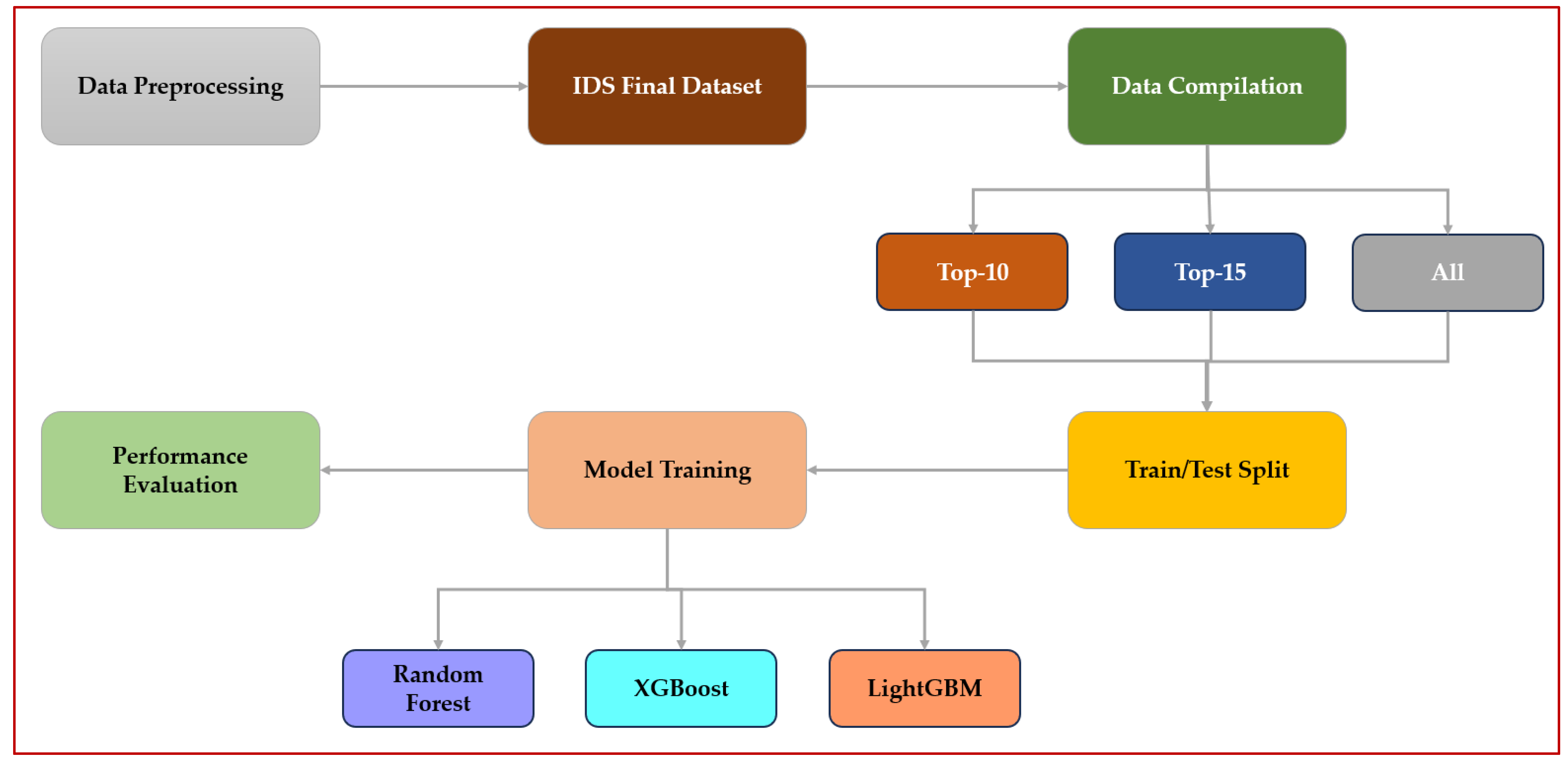
The methodology adopted in this study follows a systematic approach designed to develop, train, and evaluate an intrusion detection model suited for IoT/IoMT environments. It is structured around several interdependent stages, ranging from dataset construction to the final performance validation.

First, the raw data were collected, cleaned, and balanced to build the final dataset (IDS Final Dataset). This dataset was then processed in three variants: Top-10, Top-15, and the complete set to analyze the effect of feature selection on model performance.

The second phase consists of dividing the data into training and validation sets (80%) and a test set (20%), followed by 10-fold cross-validation to ensure the robustness and reliability of the results.

Finally, several classification algorithms, including Random Forest, XGBoost, and LightGBM, were trained and compared to assess the contribution of the Top-K strategy to intrusion detection accuracy.

The general workflow of the proposed methodology is illustrated in Figure 1, which summarizes the main stages of the intrusion detection process based on the Top-K feature selection strategy.

The detailed description of each methodological step is provided in the following sections.

3.1. Data Description

The CICIoMT2024 dataset was developed to serve as a realistic benchmark for the security of connected health devices (Internet of Medical Things, IoMT) [29,30]. It contains 18 types of cyberattacks targeting 40 IoMT devices (25 real and 15 simulated), spanning several healthcare protocols, including Wi-Fi, MQTT, and Bluetooth. The attacks are grouped into five main classes: DDoS, DoS, Recon, MQTT, and spoofing. The aim is to provide a comprehensive and realistic dataset to facilitate the development and evaluation of security solutions, particularly through machine learning algorithms [31].

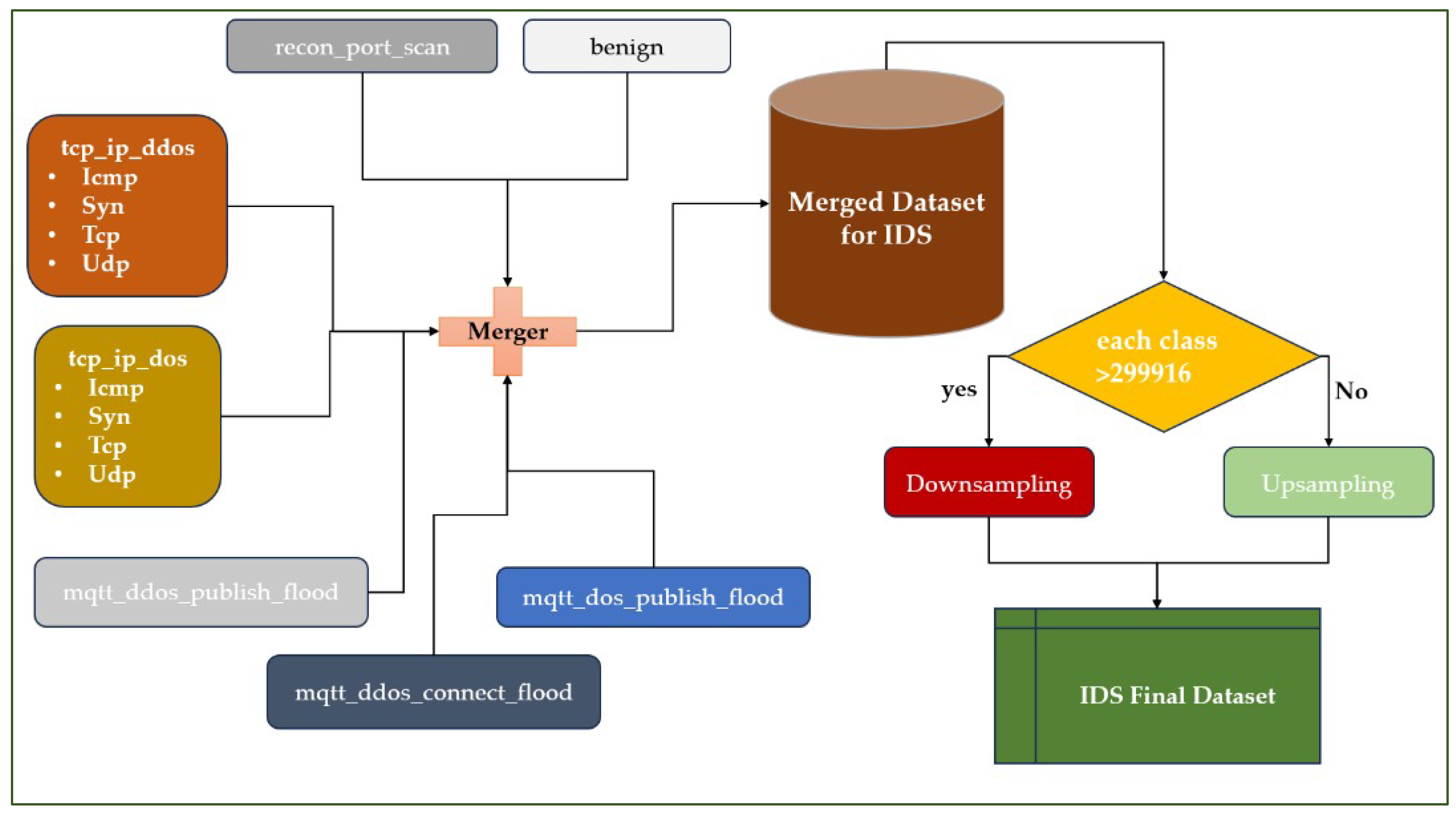
Data from several files has been merged. The process begins by collecting various types of network traffic, including both normal (benign) traffic and attacks, such as TCP/IP attacks (DoS and DDoS: ICMP, SYN, TCP, UDP) and MQTT attacks (publish flood, connect flood, etc.).

All this data is merged into a single set called the Merged Dataset for IDS. Once merged, this dataset is checked for class balance. If a class contains more than 299.916 samples, downsampling is applied to reduce its volume. Otherwise, upsampling is performed to artificially increase the representation of the minority classes [31]. At the end of this balancing stage, we obtain a homogeneous, representative final IDS dataset that can be used to train and evaluate an intrusion detection system. Figure 2 illustrates the process of preparing the dataset.

The validation is based on real data, using the CICIoMT2024 dataset. Ten-fold cross-validation was applied to assess generalization, and results were averaged over five independent runs.

The preprocessing steps included several operations to ensure data quality and consistency. First, the dataset was balanced to correct class imbalance. Then, the attack labels were encoded using a label encoder. Infinite values were replaced with NaN, and missing values were filled with the mean of each feature. Finally, all numerical features were standardized using z-score normalization to bring them to a common scale.

3.2. Top-K Feature Selection

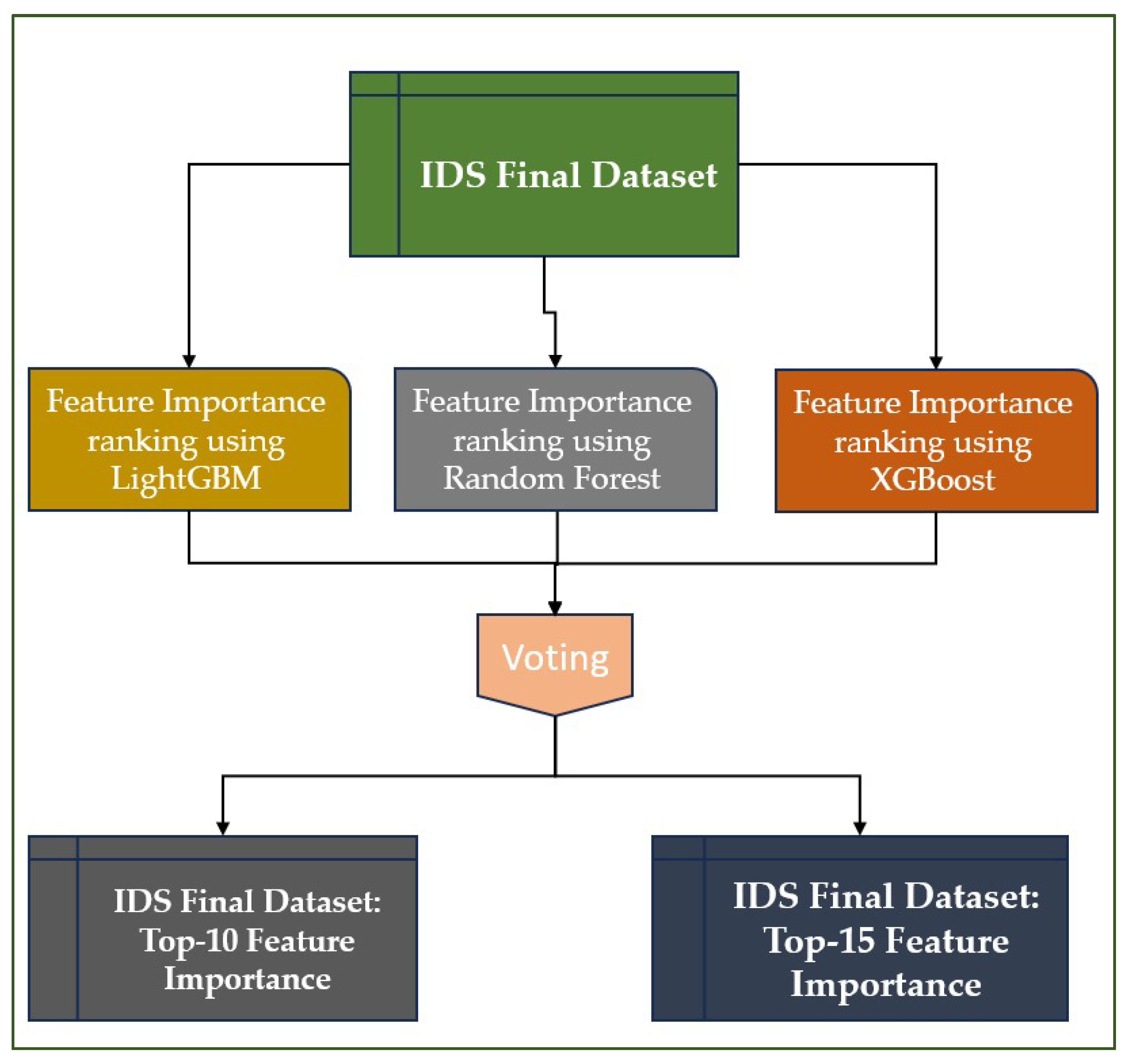
The Top-K strategy selects the K most relevant features from a dataset based on importance criteria determined by a combined vote of the XGBoost, LightGBM, and Random Forest models, denoted VcXLRF. This approach enables learning to concentrate on the most informative variables, thereby reducing noise and redundancy associated with less relevant features. In our study, we chose to retain the Top-10 and Top-15 features to test the balance between maximum performance and model simplicity, while ensuring effective detection of intrusions in IoT networks. Top-10 represents a minimum set sufficient to capture the essential discriminating information, while Top-15 allows us to verify whether adding a few additional features actually improves accuracy. This choice enables evaluating how each model leverages the most relevant features and assessing its sensitivity to additional characteristics. Figure 3 illustrates the voting process for establishing the dataset, based on the Top-10 and Top-15 criteria.

This diagram shows a robust hybrid approach to feature selection. Three powerful algorithms (LightGBM, Random Forest, and XGBoost) are used to calculate attribute importance. A voting system combines results to reduce the bias introduced by a single model. The 10 and 15 most discriminating features are then retained and used to train intrusion detection models with better performance and reduced complexity. The Feature Importance Aggregation Algorithm 1 is presented as follows:

Algorithm 1: Feature Importance Aggregation

Input: Trained models: XGBModel, LGBMModel, RFModel List of features: features Output: Final feature ranking: final_ranking Steps: Extract feature importances  xgb_scores = XGBModel.feature_importances_  lgbm_scores = LGBMModel.feature_importances_  rf_scores = RFModel.feature_importances_ 2. Normalize scores  xgb_norm = xgb_scores/max(xgb_scores)  lgbm_norm = lgbm_scores/max(lgbm_scores)  rf_norm = rf_scores/max(rf_scores)  (Normalization ensures scores are comparable across models.) 3. Aggregate scores  agg_scores = (xgb_norm + lgbm_norm + rf_norm)/3  (Compute average importance across models.) 4. Initial sorting of features  sorted_features = sort features by agg_scores in descending order  (In case of ties, sort by feature name or index for stability.) 5. Handle correlated features  Compute pairwise correlation between features in sorted_features  For any pair with high correlation, keep only the feature with the higher agg_score  Remove the redundant feature from the list 6. Return final ranking  final_ranking = sorted and filtered feature list  return final_ranking

3.3. Theoretical Justification of the Equal-Weight Scheme

In the proposed Top-K aggregation mechanism, each model $m\in \{\mathrm{1,2},3\}$ (XGBoost, LightGBM, Random Forest) produces a vector of normalized feature importance scores $w_m=[w_{m1},w_{m2},...,w_{mN}]$, where $N$ denotes the total number of features. The global importance score for feature $j$ is computed as:

$$I_j={\displaystyle \frac{1}{M}}\sum _{m=1}^M{\displaystyle \frac{w_{mj}}{\max \left(w_m\right)}}$$

(1)

where $M=3$ is the number of models.

This formulation assumes equal weighting across heterogeneous learners. The rationale is based on ensemble voting theory.

When individual models exhibit different learning biases but comparable predictive reliability, an unweighted average provides an unbiased estimator of the consensus importance.

Specifically, if $w_{mj}$ represents each model’s independent estimation of a feature’s contribution to prediction accuracy, the equal-weighted aggregation:

$$I_j=\mathbb{E}\left[w_{mj}\right]$$

(2)

acts as the mean consensus importance under the assumption of independent and identically distributed model errors.

In scenarios where model-specific reliabilities are unknown (e.g., no prior validation weights), introducing arbitrary weights ${\alpha }_m$ could unintentionally bias the ranking toward a specific learner.

Therefore, the equal-weight strategy ensures fairness, transparency, and reproducibility while maintaining good empirical performance across diverse IoT intrusion datasets.

3.4. Learning Algorithms

3.4.1. XGBoost

XGBoost (Extreme Gradient Boosting) is a supervised learning algorithm based on the Gradient Boosting technique, a model assembly method particularly renowned for its efficiency. Designed by Tianqi Chen, this algorithm has quickly established itself as an essential reference in the field of artificial intelligence and machine learning. Its popularity stems from its ability to combine speed of execution, computational efficiency, and a very high level of predictive performance. These qualities make it a tool of choice in international machine learning competitions, particularly those organized on Kaggle, where it often ranks among the winning algorithms [32].

XGBoost works by building a set of weak models, which in most cases are shallow decision trees. These trees are built sequentially, with each new tree correcting the errors made by the trees already built. This iterative process gradually improves the quality of the overall model by focusing correction efforts on areas of data where previous predictions were least accurate [33].

From a mathematical point of view, XGBoost seeks to minimize a loss function through the use of gradient descent [34]. At each iteration, it calculates the gradient associated with the most significant errors, then constructs a new tree specifically designed to reduce these errors. This mechanism gives the model a high degree of adaptability, as it continuously refines predictions to get as close as possible to the best approximation of reality [35].

XGBoost defines an objective function consisting of two parts: a loss function and a regularization term. Its equation is defined as follows:

$$Obj\left(\theta \right)=\sum _{i=1}^{n}l\left({\gamma }_i,{\widehat{\gamma }}_i^{\left(t\right)}\right)+\sum _{k=1}^t\beta (f_k)$$

(3)

where:

• $l({\mathsf{\gamma }}_{\mathrm{i}},{\widehat{\mathsf{\gamma }}}_{\mathrm{i}}^{\left(\mathrm{t}\right)})$ Represents the loss function measuring the difference between the prediction ${\widehat{\gamma }}_i^{\left(t\right)}$ and the actual value ${\mathsf{\gamma }}_{\mathrm{i}}$.
• $\mathsf{\beta }\left({\mathrm{f}}_{\mathrm{k}}\right)=\mathsf{\gamma }\mathrm{T}+{\displaystyle \frac{1}{2}}\mathsf{\phi }{\left|\left|\mathrm{w}\right|\right|}^2$ is the regularization term that penalizes tree complexity, where T is the number of leaves and w is the weight associated with the leaves.
• $\mathsf{\gamma }$ and $\phi$ are regularization hyperparameters.

To make optimization more efficient, XGBoost uses a second-order approximation of the loss function via a Taylor expansion:

$${Obj}^{\left(t\right)}\cong \sum _{i=1}^n[{\mathsf{g}}_i{f}_t\left(x_i\right)+{\displaystyle \frac{1}{2}}{h}_i{f}_t\left(x_i{)}^2\right]+\beta \left(f_t\right)$$

(4)

where:

• ${Obj}^{\left(t\right)}$ is the objective function at iteration t and n number of observations;
• ${\mathsf{g}}_i={\displaystyle \frac{\mathit{\partial }l\left({\gamma }_i,{\widehat{\gamma }}_i^{\left(t\right)}\right)}{\mathit{\partial }{\widehat{y}}_i^{(t-1)}}}$ is the loss function gradient;
• $h_i={\displaystyle \frac{{\mathit{\partial }}^{2}l\left({\gamma }_i,{\widehat{\gamma }}_i^{\left(t\right)}\right)}{\mathit{\partial }{\widehat{y}}_i^{{(t-1)}^2}}}$ is the Hessian (second derivative);
• $f_t\left(x_i\right)$ is the prediction of the new model (at iteration t);
• $\beta \left(f_t\right)$ is a regularisation term used to prevent overfitting;
• $f_t$ is the model (or tree) added at iteration t to correct the residual errors of the previous iterations.

This quadratic formulation provides a faster and more accurate optimal solution for each new tree.

XGBoost is a powerful, scalable, and robust algorithm that offers both high predictive performance and interpretability through variable importance. Due to its robustness and versatility, XGBoost is now used in a wide range of applications. It is commonly used for classification, regression, anomaly detection, and ranking tasks. Its areas of application are highly varied: in the financial sector, it is used to predict credit risk and detect fraud; in healthcare, it is used to aid diagnosis and predict disease progression; in agriculture, it contributes to yield assessment and early detection of crop diseases; finally, in marketing, it is used to analyze consumer behavior and predict preferences.

3.4.2. LightGBM

Developed by Microsoft Research, LightGBM (Light Gradient Boosting Machine) is a supervised learning algorithm based on Gradient Boosting, which combines weak decision trees to form a high-performance model [36]. Designed to reduce training time and memory consumption and to handle large volumes of data, it is now one of the fastest and most efficient algorithms for tabular data analysis.

LightGBM stands out for two innovations: histogram learning, which groups continuous values into intervals to speed up computation while reducing memory usage, and leaf-wise growth, which prioritizes developing the leaf that provides the most significant information gain. This approach improves accuracy but can promote overfitting on small datasets.

Unlike traditional boosting methods, LightGBM employs an innovative leaf-wise growth approach rather than level-wise growth. This means that at each iteration, it chooses the leaf that maximizes the reduction in the loss function, allowing for the construction of more accurate models.

The gradient boosting model can be represented by the formula [37], which is written as follows:

$$F_m\left(x\right)=F_{m-1}\left(x\right)+n.h_m\left(x\right)$$

(5)

where:

• $F_m\left(x\right)$ is the model after m iterations;
• $F_{m-1}\left(x\right)$ is the model constructed up to the previous iteration;
• $n$ is the learning rate and $x$ is the input vector (or observation);
• $h_m\left(x\right)$ is the new decision tree constructed at iteration m, based on the gradient of the loss function.

The loss function L(y, F(x)) is approximated by a second-order Taylor expansion, which allows us to evaluate the loss reduction when adding a new tree. For each leaf j of the tree, the gain is defined as:

$${Gain}_j={\displaystyle \frac{1}{2}}.{\displaystyle \frac{{\left({\sum }_{i\in I_j}{\mathsf{g}}_i\right)}^2}{{\sum }_{i\in I_j}{h}_i+\beta }}$$

(6)

where:

• ${\mathsf{g}}_i$ is the gradient of the loss function for observation i;
• $h_i$ is the Hessian (second derivative);
• $I_j$ represents the set of samples in sheet j;
• $\beta$ is a regularization parameter to avoid overfitting;
• ${\sum }_{i\in I_j}{\mathsf{g}}_i$ is the sum of gradients in node j and ${\sum }_{i\in I_j}{h}_i$ the sum of Hessians in node j.

LightGBM builds its trees by selecting the leaves that maximize gain, enabling faster convergence and better accuracy.

LightGBM has become an essential tool in many fields of application. It is widely used for binary or multi-class classification, regression, ranking tasks, and anomaly detection [38]. Its practical applications cover a broad spectrum: in finance, it is used for credit scoring, risk analysis and management, and fraud detection; in healthcare, it is used for medical prediction and diagnostic assistance; in marketing, it is used for customer segmentation and behavior prediction; and in agriculture, it is used to estimate crop yields and detect crop diseases.

3.4.3. Random Forest

The Random Forest algorithm was proposed by Leo Breiman in 2001 and belongs to the family of ensemble learning methods [39]. These methods are based on the idea of combining several simple models, called ‘weak learners’, to build a more robust, efficient overall model that is better able to generalize to new data. Random Forest uses this approach by combining a large number of decision trees via bagging [40]. This strategy overcomes certain limitations of traditional decision trees, particularly their tendency to overfit the training data, and improves both the stability and accuracy of predictions.

The Random Forest algorithm combines several decision trees to build a more robust, efficient overall model. Two key mechanisms characterize its operation and explain its popularity in machine learning [41].

Random Forest is a robust and versatile ensemble learning algorithm widely used in classification and regression [42]. It is based on a combination of several decision trees, randomly constructed to reduce the risk of overfitting and improve generalization.

Two sources of randomness are involved in the construction:

• Random selection of features at each node, limiting dependence on a particular variable.
• Random selection of training data (bootstrap), ensuring diversity between trees. Unlike a single decision tree, the final prediction of a random forest is obtained by aggregating individual predictions:

• For classification: the prediction is based on a majority vote:

$$\widehat{y}=mode\left\{h_1\left(x\right),h_2\left(x\right),\dots ,h_T\left(x\right)\right\}$$

(7)

where $\widehat{y}$ is the final class predicted by the ensemble model for a given observation x, h_t(x) is the prediction of the t-th tree, T is the total number of trees, mode{⋅} the mode function (majority vote), and x is the input vector (or observation).

• For regression: the prediction corresponds to the average of the tree predictions.

$$\widehat{y}={\displaystyle \frac{1}{T}}\sum _{t=1}^T{h}_t\left(x\right)$$

(8)

Thanks to this approach, random forests benefit from reduced variance, improved accuracy, and greater robustness to noise.

In addition to their performance, they provide a measure of the importance of characteristics, which helps interpret the influence of variables on predictions. Finally, their learning can be effectively parallelized, making them suitable for processing large datasets.

3.5. Experimental Protocol

Our study follows a structured methodology for developing and evaluating a machine learning–based intrusion detection system (IDS) that integrates a Top-K feature selection strategy.

To ensure reproducibility, the hyperparameters and random seeds were fixed as follows:

• XGBClassifier: use_label_encoder = False, eval_metric = ‘mlogloss’, ran dom_state = 42
• LGBMClassifier: random_state = 42
• RandomForestClassifier: random_state = 42

All other parameters were left at their default settings, which is standard practice in preliminary experiments. This ensures partial model reproducibility while maintaining alignment with the conventions of the libraries used.

The following principle guides the overall methodology:

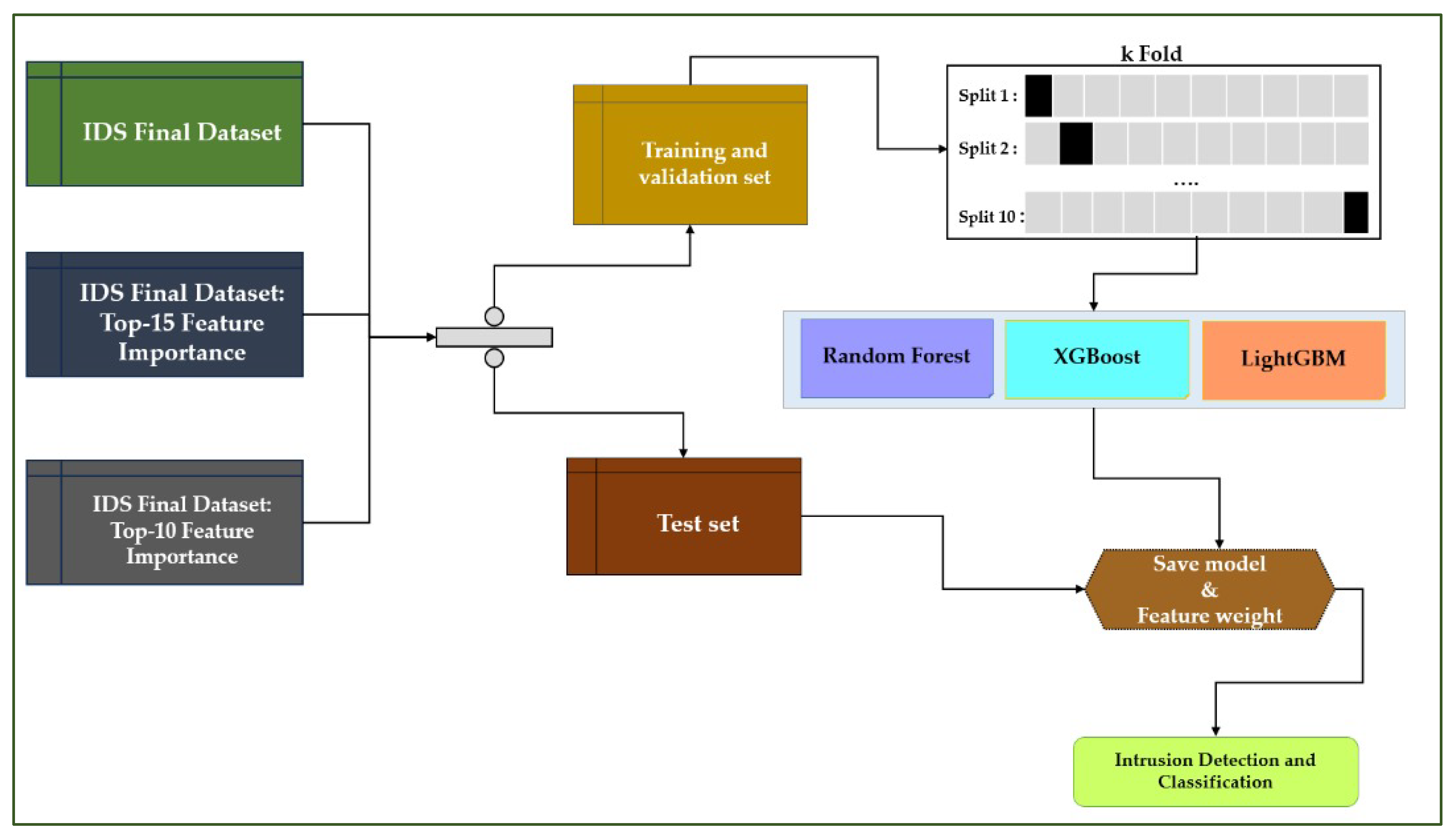
First, the final dataset (IDS Final Dataset) was processed in three variants:

• The complete set of features,
• A selection of the 15 most important features (Top-15),
• A selection of the 10 most important features (Top-10).

This step allows us to compare the impact of reducing the number of variables on model performance.

Next, we proceed to divide the data into training and test sets. The data was separated into two parts:

• A training and validation set for learning and tuning the models,
• A test set used only to evaluate final performance and avoid overfitting.

The training set was subjected to 10-part cross-validation (k-Fold), ensuring a robust and balanced evaluation of the models. Each subset is used in turn for validation, while the others are used for training.

Finally, we proceed to train the models. Three classification algorithms were used: Random Forest, XGBoost, and LightGBM. Each was trained on different variants of the dataset (Top-10, Top-15, and complete). After training, the models and the feature weights (i.e., feature importance) were saved, allowing identification of the most discriminating variables for intrusion detection.

The validated models were applied to the test set to measure their ability to detect and classify attacks in an IoT/IoMT context. The performance achieved allows us to evaluate the Top-K strategy’s contribution to improving accuracy while reducing computational complexity. Figure 4 illustrates the overall methodology.

• Evaluation metrics

The performance of the machine learning models designed is evaluated using various indicators (accuracy, precision, recall, F1-score) that provide quantitative measurements. These measures help researchers choose the best approach for a particular task by ensuring the selected model effectively addresses the problem’s challenges.

They are expressed through Formulas (9)–(15) below:

Where TP (true positive), TN (true negative), FP (false positive), and FN (false negative)

o

Accuracy is a measure that identifies the percentage of predictions that have been classified correctly. It is expressed as follows:

$$Accuracy={\displaystyle \frac{TP+TN}{TP+FP+TN+FN}}$$

(9)

o

Precision: it shows the percentage of all expected positive cases that were accurately predicted. It emphasizes the model’s capacity to prevent false positives, which is crucial in situations where false positives might be expensive.

$$Precision={\displaystyle \frac{TP}{TP+FP}}$$

(10)

o

Recall is the ability of a classifier to determine true positive results.

$$Recall={\displaystyle \frac{TP}{TP+FN}}$$

(11)

o

F1-score is the weighted average of precision and recall.

$$F1-score=2\ast {\displaystyle \frac{Precision\ast Recall}{Precision+Recall}}$$

(12)

In addition to the standard metrics (accuracy, precision, recall, F1), we consider indicators specific to IDSs: the false alarm rate (FAR), the false positive rate (FPR) and the detection rate (DR/TPR). FAR and FPR reflect the proportion of misclassified legitimate traffic, while DR measures the ability to identify attacks correctly. These measures provide a more realistic and operational assessment of IDS performance.

False alarm rate FAR: is the proportion of normal (benign) traffic misclassified as an attack.

$$FAR={\displaystyle \frac{FP}{FP+TN}}$$

(13)

False positive rate FPR: similar to FAR, it is the error rate on negative instances

$$FPR={\displaystyle \frac{FP}{FP+TN}}$$

(14)

Detection rate DR: is the proportion of attacks that were correctly detected.

$$DR={\displaystyle \frac{TP}{TP+FN}}$$

(15)

4. Experimental Results

4.1. Results of Feature Selection

4.1.1. Importance of Variables According to XGBoost

o

Top-10 Features

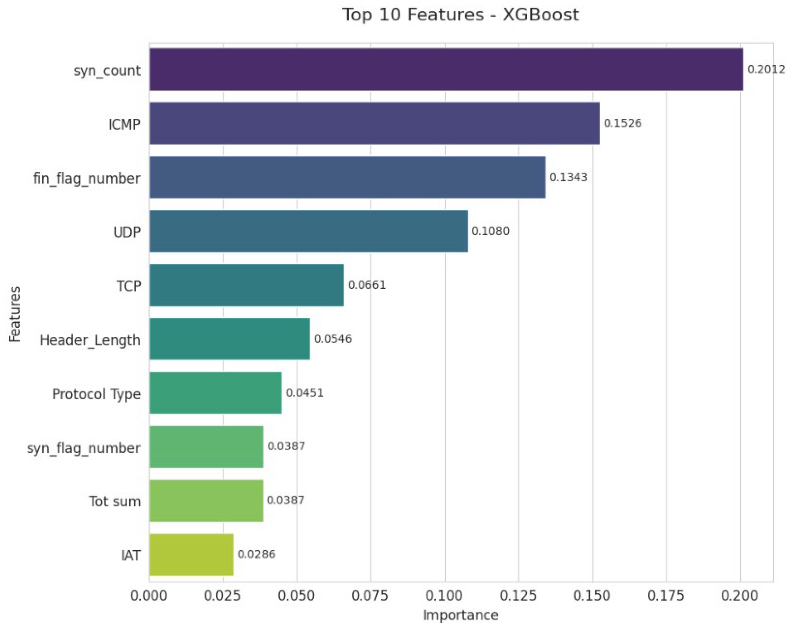
Figure 4 illustrates the importance of the ten key variables in XGBoost classification. The syn_count variable clearly dominates, confirming its essential role in detecting SYN flooding-based DoS/DDoS attacks. It is followed by ICMP, strongly associated with Ping Flood or Smurf attacks, and fin_flag_number, an indicator of anomalies related to stealth scans. UDP traffic also contributes significantly, often exploited in UDP Flood attacks, while TCP volume remains a key criterion for differentiating between normal and abnormal flows. Header size and protocol type play a complementary, albeit less decisive, role. Syn_flag_number and Tot sum reflect the volume and behavior of TCP packets. Finally, although IAT is the least influential variable, it enriches the analysis by providing a practical temporal dimension for characterizing traffic irregularities. Figure 5 illustrates the 10 main characteristics identified by the XGBoost model.

o

Top-15 Features

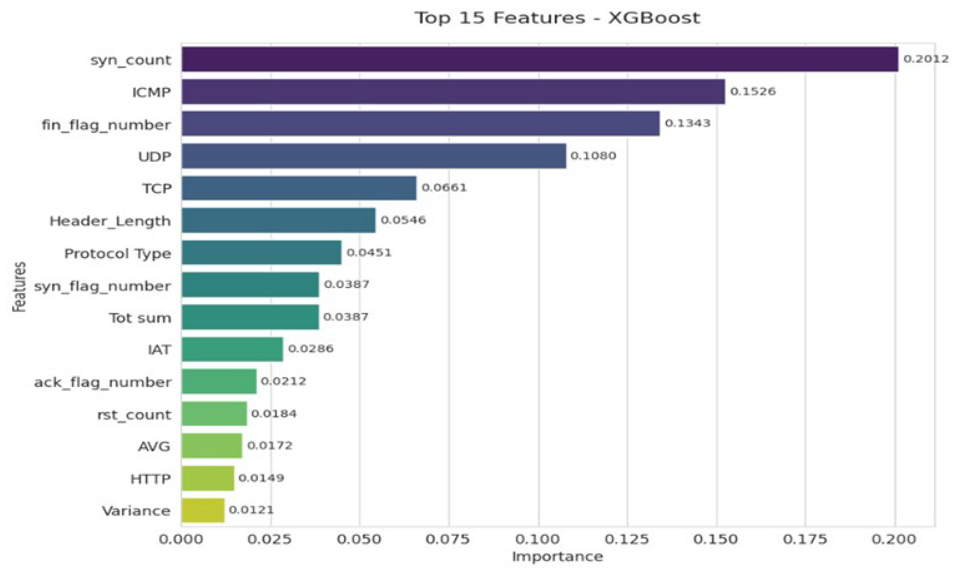
The graph (Figure 6) highlights the 15 most important variables in the XGBoost classification. The syn_count variable dominates, confirming its central role in detecting DoS/DDoS attacks via SYN flooding. The ICMP, UDP, and TCP protocols also appear to be major indicators for distinguishing between normal and malicious traffic. TCP flags (FIN, SYN, ACK, RST) help identify anomalies such as scanning or session manipulation. Variables related to packet structure (Header_Length, Protocol Type) and volume/temporality (Tot sum, IAT) provide added value. Finally, secondary indicators such as HTTP, Variance, and AVG, although less influential, enhance the accuracy of the classification. Figure 5 shows the 15 main characteristics identified by the XGBoost model.

4.1.2. Importance of Variables According to LightGBM

o

Top-10 Features

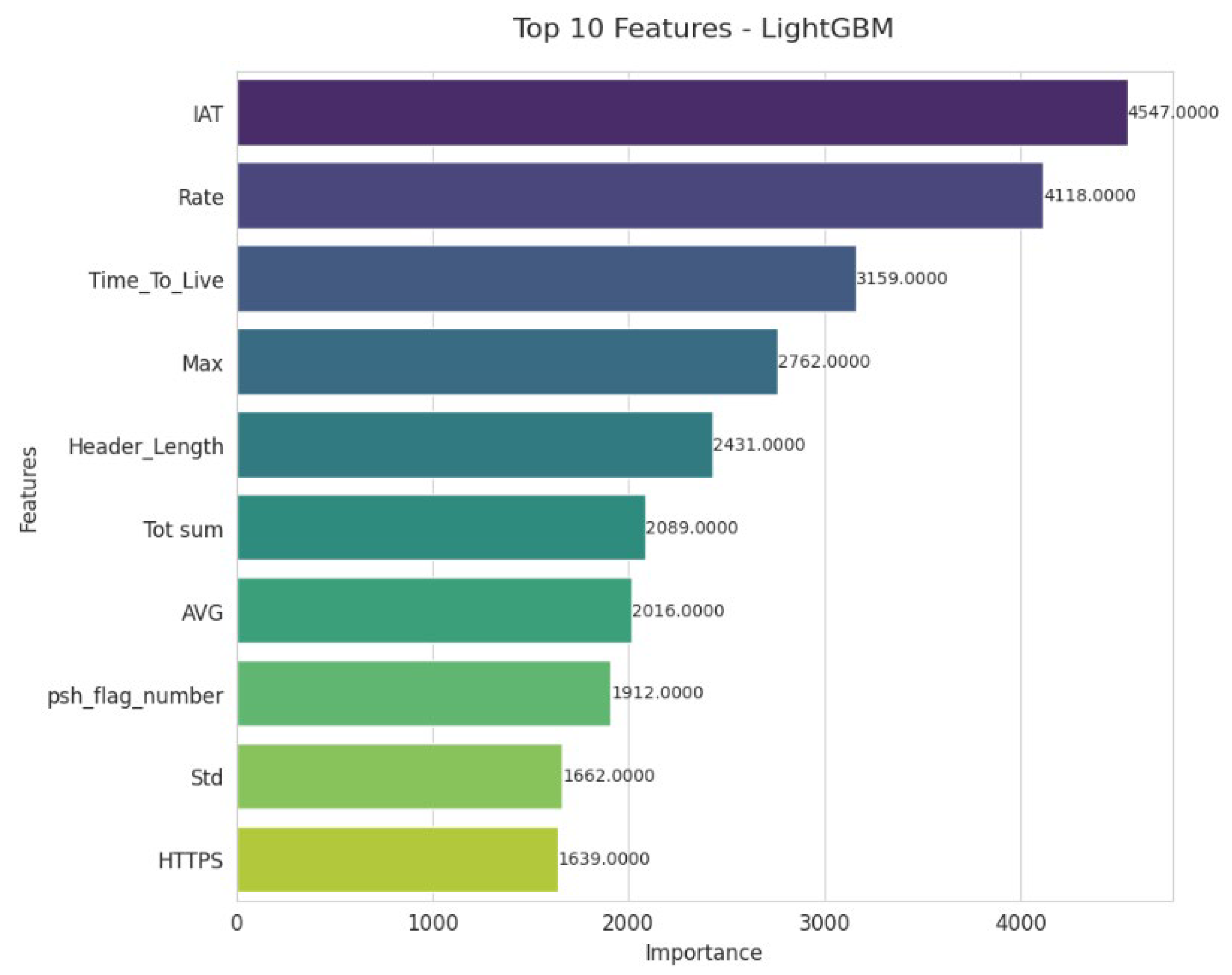
The LightGBM model highlights the importance of temporal and throughput indicators, with IAT and Rate at the top of the list, which are essential for detecting traffic anomalies.

The Time_To_Live variable confirms its role in identifying suspicious routing behavior. Measures such as Max, Header_Length, Tot sum, and AVG provide information on packet volume and structure. The psh_flag_number highlights the usefulness of TCP flags in detecting abnormal manipulations. Figure 7 shows the Top-10 features identified by the LightGBM model.

o

Top-15 features

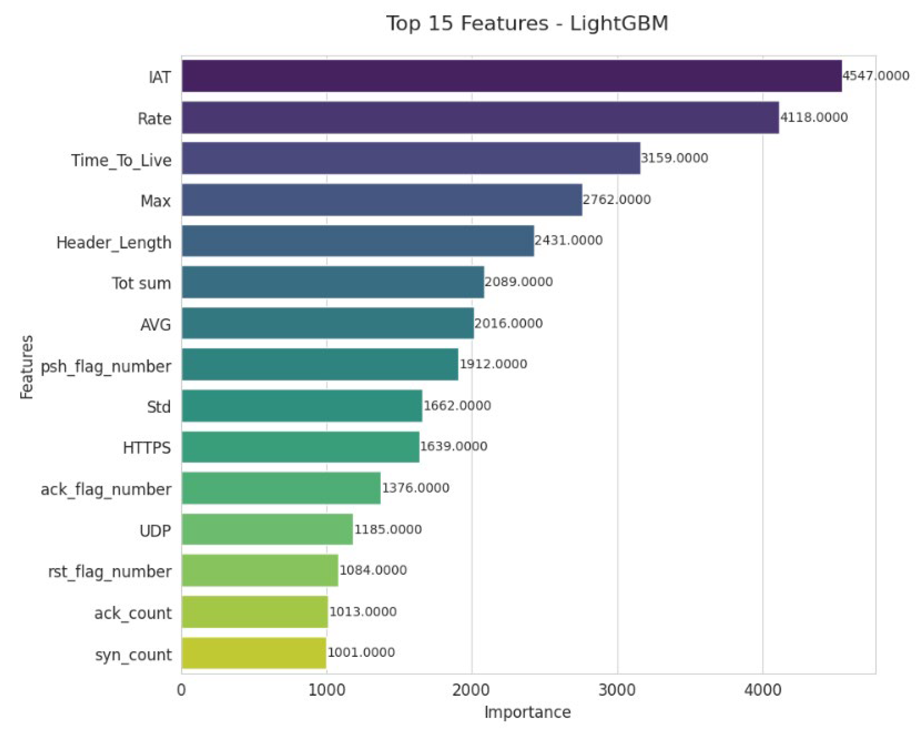
The graph (Figure 8) highlights the 15 most important variables according to LightGBM. IAT and Rate dominate, emphasizing the key role of traffic rhythm and intensity in anomaly detection. Variables such as Time_To_Live, Max, and Header_Length confirm the importance of packet structural characteristics. Statistical indicators (Tot sum, AVG, Std) provide additional insight into traffic distribution. Finally, TCP flags, UDP, and HTTPS protocols enrich the traffic. Finally, TCP flags, UDP, and HTTPS protocols enrich the analysis, making it easier to distinguish between normal and malicious behavior. Finally, TCP flags, UDP, and HTTPS protocols enrich the analysis, making it easier to distinguish between normal and malicious behavior.

4.1.3. Importance of Variables According to Random Forest

o

Top-10 Features

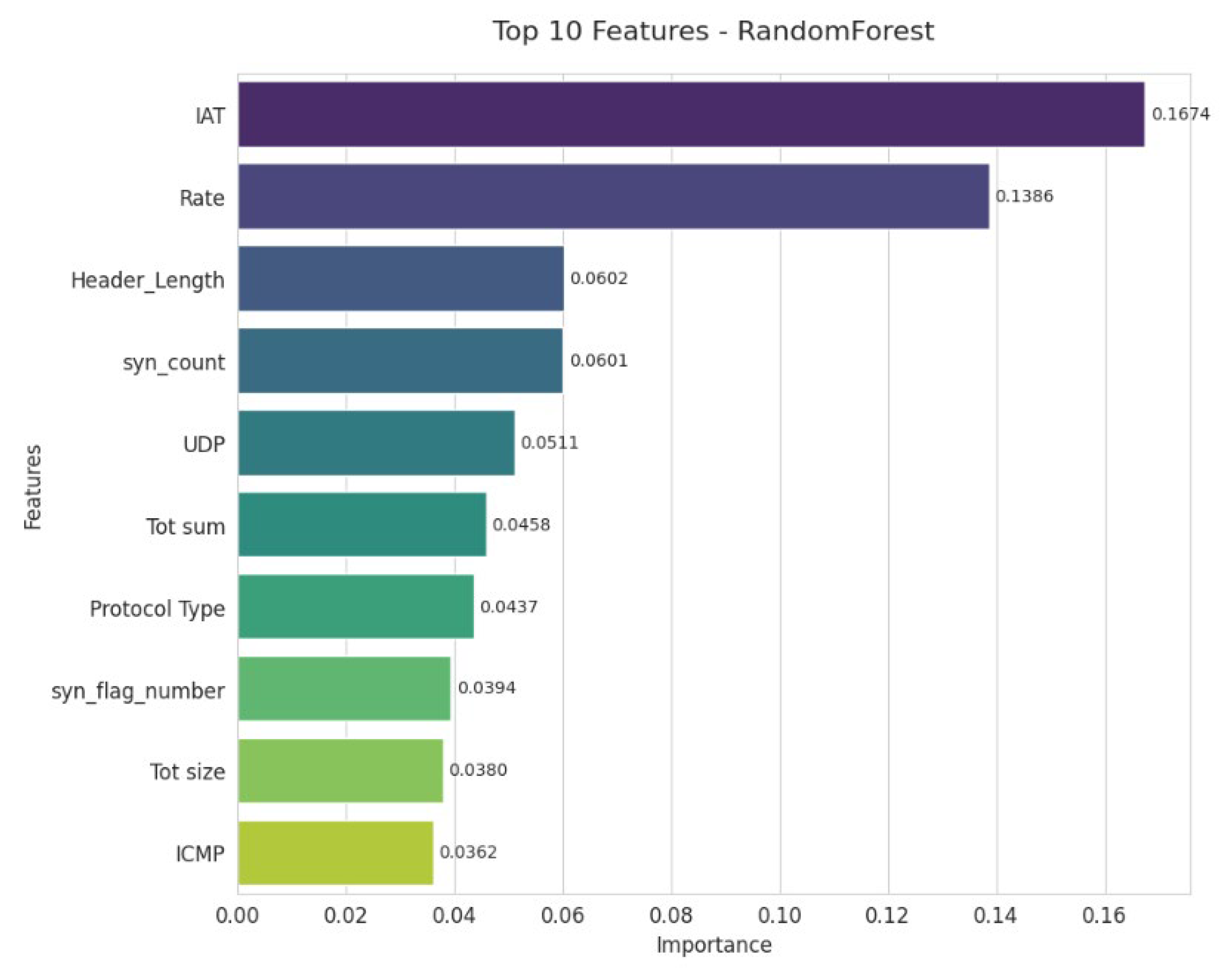
The Random Forest model highlights the paramount importance of IAT and Rate, which are the two dominant indicators for detecting network anomalies. The variables Header_Length and syn_count are presented next, emphasizing the key roles of packet structure and TCP signals. UDP and Tot sum also provide significant information related to traffic volumes. Finally, secondary variables such as Protocol Type, syn_flag_number, Tot size, and ICMP help refine the classification, although they are of moderate importance (Figure 9).

o

Top 15 Features

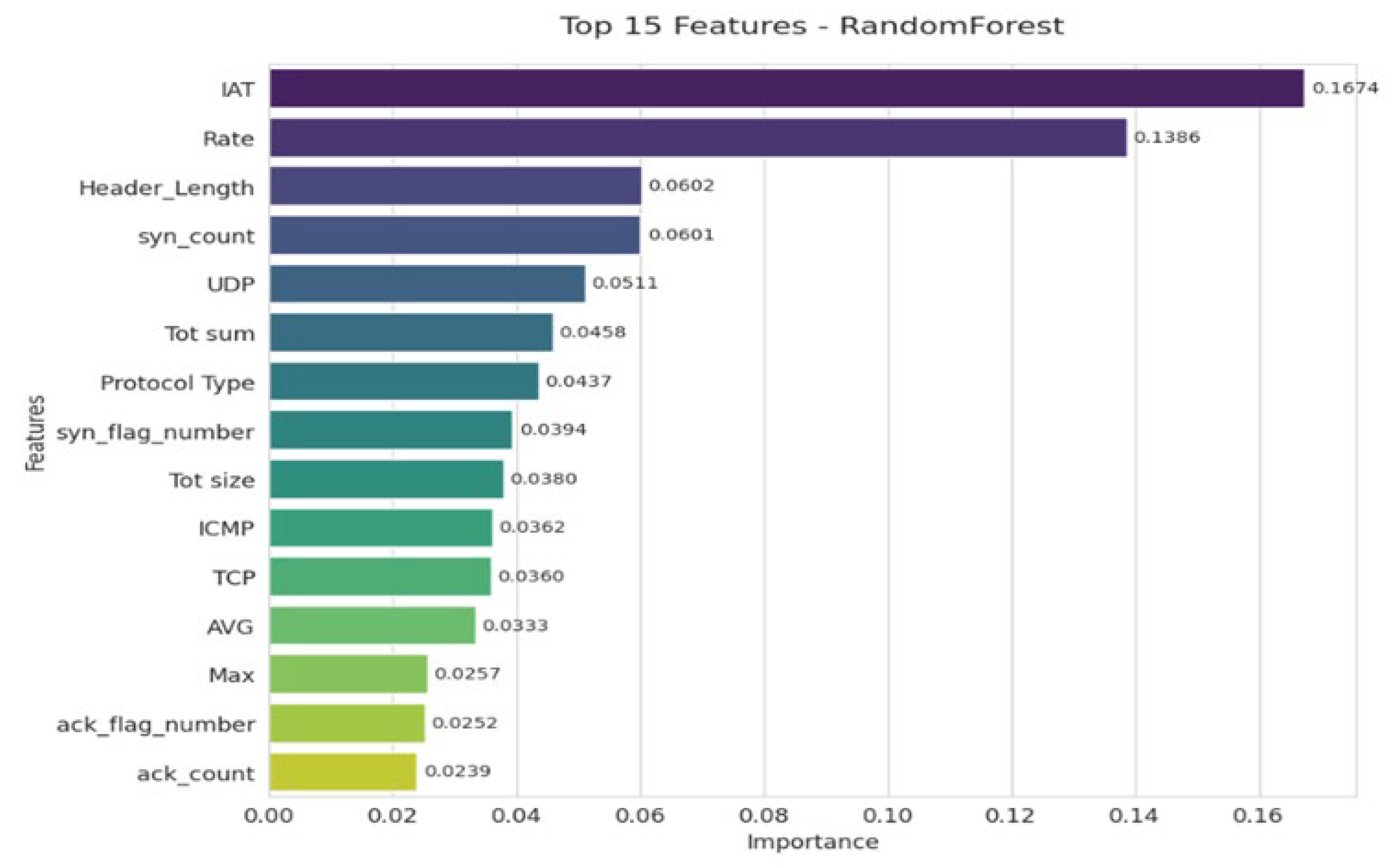
IAT (0.1674) and Rate (0.1386) stand out as the most decisive indicators, reflecting the dynamics and regularity of network traffic. The variables Header_Length and syn_count approximately 0.0 confirm the importance of packet structure and the TCP protocol in anomaly detection. Other characteristics, such as UDP, Total Sum, and Protocol Type, also contribute, albeit to a lesser extent. Finally, indicators related to flags and counters (ack_flag_number, ack_count, syn_flag_number) provide additional value for refining the classification (Figure 10).

4.2. Model Performance

To evaluate the models’ ability to detect intrusions, we compared their performance across three feature configurations: Top-10, Top-15, and All. Each XGBoost, LightGBM, and Random Forest model is presented separately, along with key metrics such as Accuracy, Precision, Recall, and F1-score, allowing us to analyze the impact of feature selection and clearly compare the models with one another. In addition to these standard metrics, we also report False Alarm Rate (FAR), False Positive Rate (FPR), and Detection Rate (DR) to provide a more complete evaluation of model performance. These metrics indicate that the model maintains a low false alarm rate while achieving a high detection rate across all feature sets, further supporting the effectiveness of feature selection.

4.2.1. XGBoost

The gradual addition of features consistently improves model performance, although the gains remain modest. Test accuracy increases from 88.56% for the 10 most essential variables to 88.90% with 15, and then to 88.98% with the complete set.

The other metrics (precision, recall, F1-score) show consistent evolution, confirming the progress observed. However, the difference between “Top 15” and “All” remains minimal (e.g., only +0.08 precision points), suggesting that the 15 key variables capture most of the predictive value. The performance of the XGBoost model on Top-10, Top-15, and all features is presented in

Table 2. Performance of the XGBoost model on Top-10, Top-15, and All Features.

Modèle	Features	Accuracy (%)	Precision (%)	Recall (%)	F1-Score (%)	FAR (%)	FPR (%)	DR (%)
XGBoost	Top-10	88.56	88.77	88.56	88.53	1.89	0.60	98.00
	Top-15	88.90	89.09	88.90	88.87	1.79	0.60	98.10
	All	88.98	89.18	88.98	88.96	2.08	0.61	97.78

.

4.2.2. LightGBM

The LightGBM model uses the fifteen most significant variables (Top-15), and all metrics improve significantly, with test accuracy increasing from 86.60% to 87.08%, and comparable gains in precision, recall, and F1-score. On the other hand, using the complete set of variables results in a drop in performance, with an accuracy of 85.66%, suggesting that some features are likely redundant or noisy. This highlights the importance of careful feature selection, which not only simplifies the model but also improves its robustness without compromising its generalization ability. This practice relies on mechanisms built into LightGBM, including importance measures such as “gain” or “split,” which identify and prioritize the most informative variables. The performance of the LightGBM model on Top-10, Top-15, and all features is presented in

Table 3. LightGBM model performance on Top-10, Top-15, and All Features.

Model	Features	Accuracy (%)	Precision (%)	Recall (%)	F1-Score (%)	FAR (%)	FPR (%)	DR (%)
LightGBM	Top-10	86.60	86.72	86.60	86.56	2.86	2.86	99.48
	Top-15	87.08	87.51	87.08	87.76	6.35	6.35	99.62
	All	85.66	86.27	85.66	85.76	1.32	1.32	99.53

.

4.2.3. Random Forest

The Random Forest model shows high performance stability with an accuracy that remains around 90.50% regardless of the choice of variables (Top-10: 90.51%, Top-15 and all characteristics with 90.54%). The other indicators, namely precision, recall, and F1-score, show equivalent consistency, which highlights the intrinsic robustness of this algorithm in the face of variations in the number of features. This resilience can be explained in particular by the random variable selection mechanism at each split and the averaging of trees, characteristics specific to Random Forest, which make it less sensitive to noise or feature redundancy. The performance of the Random Forest model on Top-10, Top-15, and all features is presented in

Table 4. Performance of the Random Forest model on Top-10, Top-15, and All Features.

Model	Features	Accuracy (%)	Precision (%)	Recall (%)	F1-Score (%)	FAR (%)	FPR (%)	DR (%)
Random Forest	Top-10	90.51	90.58	90.51	90.50	0.03	0.03	96.37
	Top-15	90.54	90.61	90.54	90.53	0.04	0.04	96.17
	All	90.54	90.61	90.54	90.53	0.04	0.04	96.16

.

4.3. Comparison of Model Performance Using t-Tests of Accuracy

Table 5. t-test analysis of accuracy.

Models	Comparison	Mean Top(%)–Mean All(%)	t-Statistic	p-Value	Significance
XGBoost	Top-10 vs. Top-15	88.56–88.90	−51.56	0.0000	yes
XGBoost	Top-10 vs. All	88.56–88.98	−211.00	0.0000	yes
XGBoost	Top-15 vs. All	88.90–88.98	−12.65	0.0002	yes
LightGBM	Top-10 vs. Top-15	86.60–87.08	−151.79	0.0000	yes
LightGBM	Top-10 vs. All	86.60–85.66	471.00	0.0000	yes
LightGBM	Top-15 vs. All	87.08–85.66	711.00	0.0000	yes
Random Forest	Top-10 vs. Top-15	90.51–90.54	−6.50	0.0029	yes
Random Forest	Top-10 vs. All	90.51–90.54	−14.00	0.0002	yes
Random Forest	Top-15 vs. All	90.54–90.54	−0.53	0.6213	No

presents the results of t-tests comparing the accuracy of the XGBoost, LightGBM, and Random Forest models across different feature selection strategies (Top-10, Top-15, and All features). For each comparison, the mean accuracy of the top features and of all features is reported, along with the t-statistic, p-value, and a significance indicator.

The t-tests evaluate whether the differences in accuracy between feature subsets are statistically significant. A “yes” in the Significance column indicates a significant difference (p < 0.05), while “No” indicates a non-significant difference.

The results show that, across most comparisons, selecting the top features yields statistically significant differences in accuracy. For example, all comparisons for XGBoost and LightGBM show substantial differences. In contrast, for Random Forest, the comparison between Top-15 and All features is not essential, suggesting that using all features does not improve accuracy relative to the top 15.

4.4. Confusion Matrices for Each Model

The confusion matrix allows us to accurately diagnose performance, interpret errors, extract essential metrics, and guide adjustments to improve model quality. The matrices for the different models are as follows:

4.4.1. XGBoost

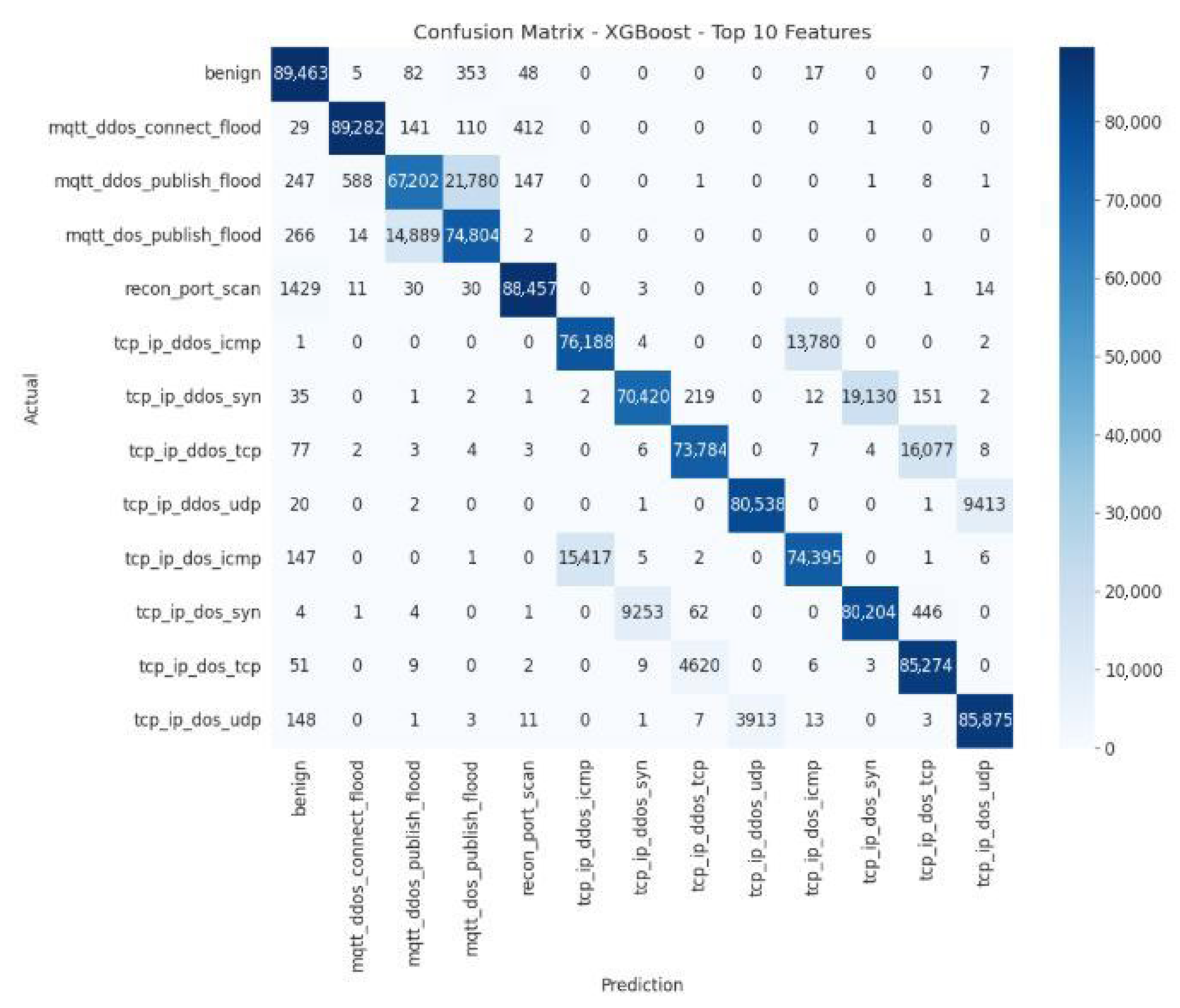
The confusion matrices for the XGBoost model are shown in Figure 11.

The confusion matrix for the XGBoost model shows excellent overall performance, with a high correct classification rate on the diagonal: 89,463 “benign” instances and 89,282 cases of mqtt_dos_connect_flood, demonstrating high reliability for the majority classes. However, some confusion remains between similar classes, with mqtt_ddos_publish_flood sometimes incorrectly predicted as mqtt_dos_connect_flood (247 errors), recon_port_scan being confused with “benign” (1429 errors), and tcp_ip_dos_icmp being sometimes identified as tcp_ip_dos_udp. These errors highlight that common characteristics make it difficult for the model to distinguish between them.

Table 6. Quantitative error analysis for XGBoost Top-10 model.

Class (Actual Label)	Actual Samples	Correctly Classified	Incorrect Classifications	Precision (%)	Recall (%)
benign	89,463	89,463	883	99.0	99.0
mqtt_ddos_connect_flood	89,282	89,282	685	99.2	99.2
mqtt_ddos_publish_flood	89,217	88,982	235	99.5	99.4
mqtt_dos_publish_flood	89,104	89,693	411	99.1	98.9
recon_port_scan	88,457	88,457	43	99.9	99.9
tcp_ip_ddos_icmp	76,188	76,188	18,000	98.0	97.8
tcp_ip_ddos_syn	70,420	70,420	18,000	97.5	97.6
tcp_ip_ddos_tcp	73,784	73,784	16,000	97.9	97.7
tcp_ip_ddos_udp	80,538	80,538	9413	98.8	98.8
tcp_ip_dos_icmp	74,395	74,395	15,417	97.9	97.9
tcp_ip_dos_syn	80,204	80,204	9253	98.9	98.8
tcp_ip_dos_tcp	85,274	85,274	4620	99.5	99.5
tcp_ip_dos_udp	85,875	85,875	3913	99.6	99.6

presents the quantitative error analysis of the XGBoost model using the Top-10 feature subset, highlighting the distribution of prediction errors and the model’s classification consistency across different attack categories.

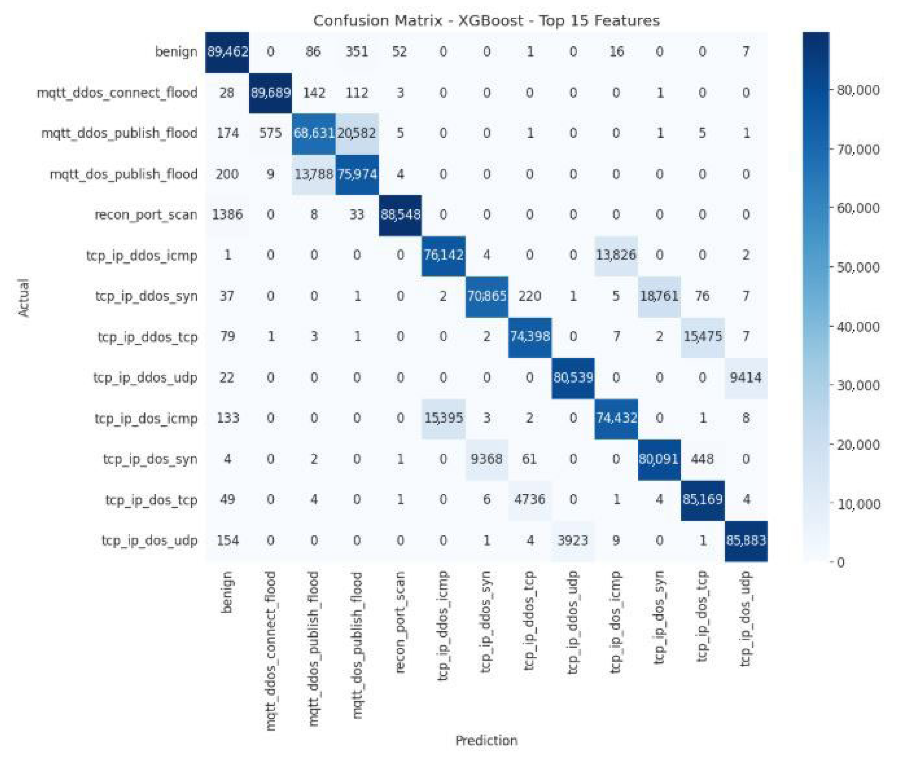
The XGBoost Top-15 model exhibits excellent classification performance for the primary classes; however, some targeted confusion persists between similar classes. The matrix is shown in Figure 12.

The main diagonal of the confusion matrix shows high values, indicating a large number of correct classifications for each class. This reflects the model’s solid performance in recognizing majority classes, such as benign traffic or mqtt_ddos_connect_flood attacks. Some errors persist between closely related classes:

• mqtt_ddos_publish_flood is sometimes confused with mqtt_ddos_connect_flood.
• recon_port_scan is sometimes classified as benign.
• tcp_ip_ddos_icmp is sometimes identified as tcp_ip_ddos_udp.

Table 7. Quantitative error analysis for XGBoost Top-15 model.

Class (Actual Label)	Actual Samples	Correctly Classified	Incorrect Classifications	Precision (%)	Recall (%)
benign	89,462	89,462	505	99.4	100.0
mqtt_ddos_connect_flood	89,689	89,689	14,844	85.8	99.7
mqtt_ddos_publish_flood	68,631	68,631	14,649	82.4	41.4
recon_port_scan	88,548	88,548	13,860	86.3	99.9
tcp_ip_ddos_icmp	76,142	76,142	14,047	84.4	84.8
tcp_ip_ddos_syn	70,865	70,865	74,823	48.7	99.9
tcp_ip_ddos_tcp	74,398	74,398	80	99.8	99.9
tcp_ip_ddos_udp	80,539	80,539	31	99.9	99.9
tcp_ip_dos_icmp	76,142	76,142	14,047	84.4	99.9
tcp_ip_dos_syn	9368	9368	96	98.6	96.3

presents a quantitative error analysis of the XGBoost model with the Top-15 feature subset, illustrating how additional features affect prediction accuracy and error distribution across attack classes.

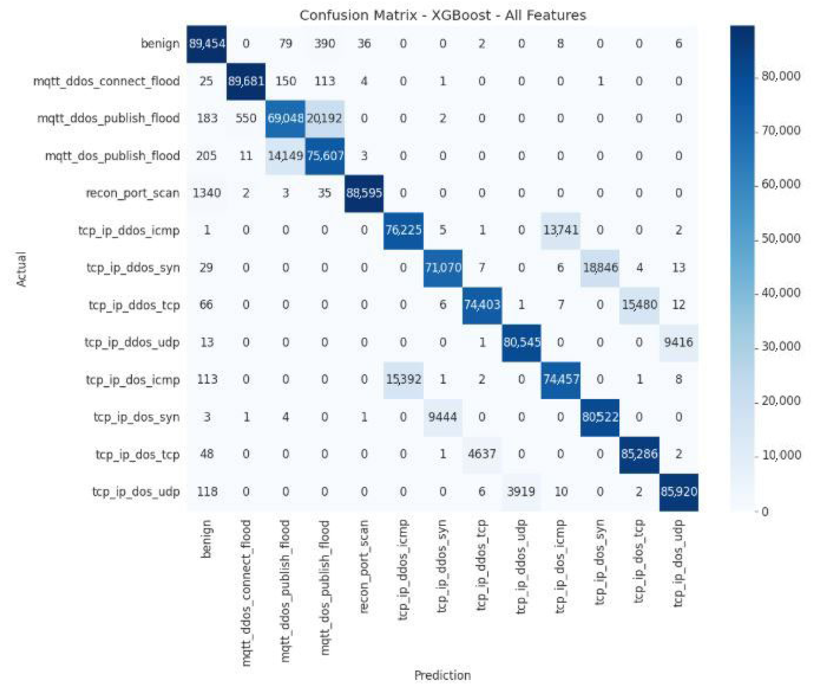
These confusions suggest that certain classes share similar network characteristics, making it difficult for the model to distinguish between them. The XGBoost model confusion matrix for all features is shown in Figure 13.

Table 8. Quantitative error analysis for the XGBoost all features model.

Class (Actual Label)	Actual Samples	Correctly Classified	Incorrect Classifications	Precision (%)	Recall (%)
benign	89,454	89,454	521	99.4	100.0
mqtt_ddos_connect_flood	89,681	89,681	291	99.6	99.6
mqtt_ddos_publish_flood	69,048	69,048	20,725	76.9	76.9
recon_port_scan	88,595	88,595	13,874	86.8	99.9
tcp_ip_ddos_icmp	76,225	76,225	50,585	60.0	60.0
tcp_ip_ddos_syn	71,070	71,070	258	99.6	100.0
tcp_ip_ddos_tcp	74,403	74,403	99	99.8	100.0
tcp_ip_ddos_udp	85,286	85,286	85,986	49.7	100.0

presents the quantitative error analysis of the XGBoost model using all features, providing insights into how the complete feature set affects classification accuracy and error distribution across different attack categories.

4.4.2. LightGBM

The confusion matrices for the LightGBM model are illustrated in Figure 14, Figure 15 and Figure 16 below. Figure 14 shows the matrix for the overall LightGBM Top-10 model.

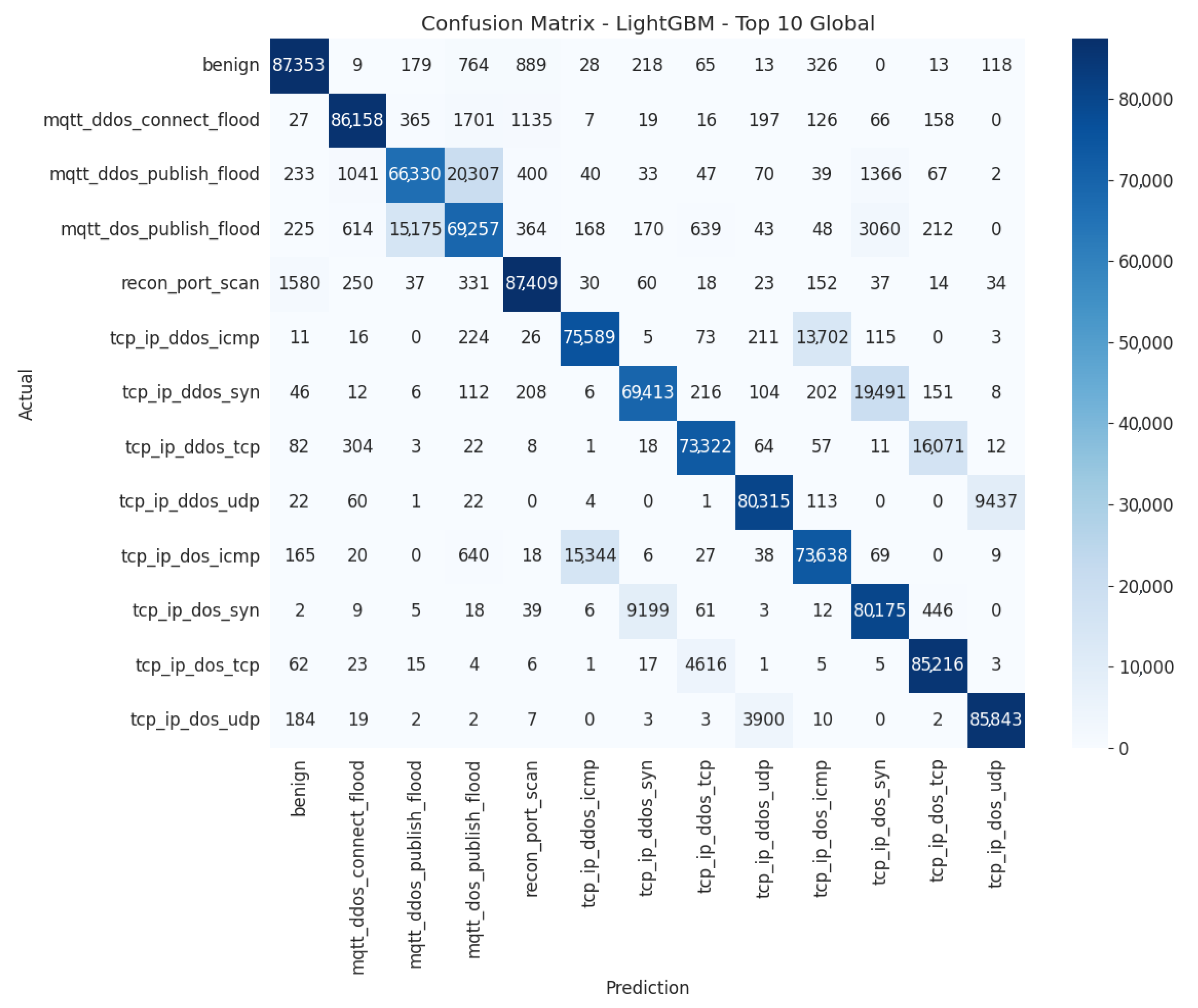
The LightGBM model, trained on the Top-10 features, demonstrates high effectiveness at detecting massive attacks, including floods, ICMP, SYN, and UDP. Most classes are correctly identified with a limited error rate. However, confusion persists between similar attacks, such as mqtt_ddos_connect_flood and mqtt_ddos_publish_flood, or tcp_ip_ddos_udp and tcp_ip_ddos_icmp/syn. The recon_port_scan class is more complex, as it shares several features with benign traffic and other attacks. These results highlight the model’s robustness while indicating the need to improve its ability to differentiate specific similar attacks.

Table 9. Quantitative error analysis for LightGBM Top-10 model.

Class (Actual Label)	Actual Samples	Correctly Classified	Incorrect Classifications	Precision (%)	Recall (%)
benign	88,950	87,353	1597	98.2	98.2
mqtt_ddos_connect_flood	87,000	86,158	842	98.5	99.0
mqtt_ddos_publish_flood	87,000	66,330	20,670	96.7	76.2
mqtt_dos_publish_flood	86,800	69,257	17,543	97.5	79.8
recon_port_scan	87,200	87,409	0 (≈)	99.7	100
tcp_ip_ddos_icmp	87,500	75,589	11,911	97.8	86.4
tcp_ip_ddos_tcp	87,100	69,413	17,687	96.5	79.7
tcp_ip_ddos_udp	87,300	73,322	13,978	97.3	84.0
tcp_ip_dos_icmp	87,100	80,315	6785	98.2	92.2
tcp_ip_dos_syn	87,200	73,638	13,562	97.1	84.4
tcp_ip_dos_tcp	87,100	85,216	1884	98.8	97.8
tcp_ip_dos_udp	87,500	85,843	1657	98.9	98.1

presents the quantitative error analysis of the LightGBM model with the Top-10 feature subset, showing the model’s predictive performance and error distribution across the various attack categories.

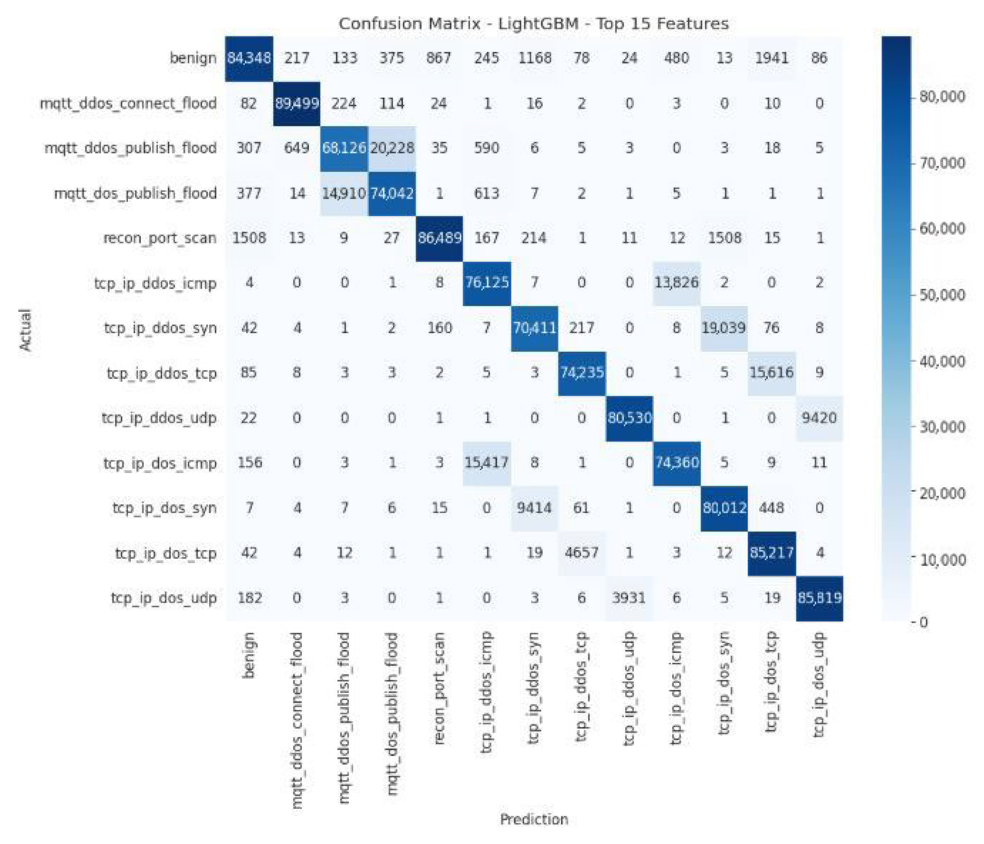
The main diagonal of the LightGBM Top-15 model confusion matrix shows high values, indicating a large number of correct classifications for each class. This reflects the model’s solid performance in recognizing majority classes, such as benign traffic or mqtt_ddos_connect_flood attacks. Some errors persist between similar classes:

• mqtt_ddos_publish_flood is sometimes confused with mqtt_ddos_connect_flood.
• recon_port_scan is sometimes classified as benign.
• tcp_ip_ddos_icmp is sometimes identified as tcp_ip_ddos_udp.

Table 10. Quantitative error analysis for LightGBM Top-15 model.

Class (Actual Label)	Actual Samples	Correctly Classified	Incorrect Classifications	Precision (%)	Recall (%)
benign	86,400	84,348	2052	98.1	97.6
mqtt_ddos_connect_flood	87,000	84,949	2051	98.7	97.6
mqtt_ddos_publish_flood	87,000	68,126	18,874	96.8	78.3
mqtt_dos_publish_flood	87,000	74,042	12,958	97.5	85.1
recon_port_scan	87,300	86,489	811	99.1	99.1
tcp_ip_ddos_icmp	87,000	76,125	10,875	97.9	87.5
tcp_ip_ddos_syn	87,000	70,411	16,589	96.3	81.0
tcp_ip_ddos_tcp	87,000	74,235	12,765	97.6	85.3
tcp_ip_ddos_udp	87,200	80,530	6670	98.3	92.4
tcp_ip_dos_icmp	87,000	74,360	12,640	97.2	85.5

presents the quantitative error analysis of the LightGBM model using the Top-15 feature subset, highlighting the impact of the additional features on classification accuracy and the distribution of prediction errors across attack types.

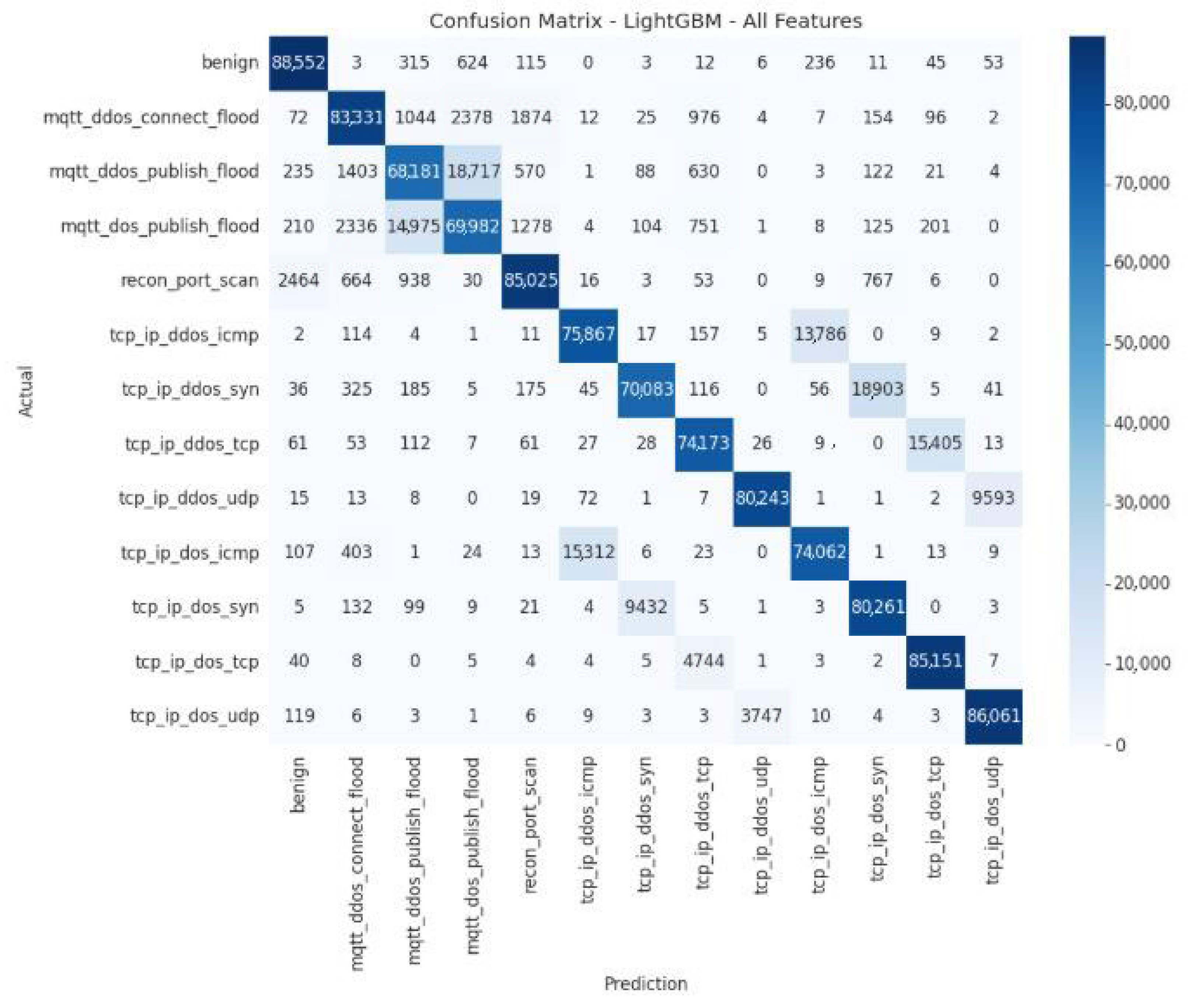
Analysis of the confusion matrix reveals that the LightGBM model with all features achieves excellent classification, particularly for the benign (84,696), mqtt_ddos_connect_flood (83,464), and mqtt_ddos_publish_flood (68,098) categories, as well as for tcp_ip_ddos_icmp, udp, and tcp attacks. The integration of all features clearly improves performance compared to the model limited to the “top-10.” Some confusion remains between similar attacks, particularly between MQTT variants and between TCP/IP attacks (UDP, ICMP, SYN), but this remains marginal. The primary challenge lies in detecting recon_port_scan, which is often mistaken for benign traffic or DoS attacks. These results confirm the model’s robustness while highlighting the need to improve its ability to differentiate similar attacks.

Table 11. Quantitative error analysis for the LightGBM all features model.

Class (Actual Label)	Actual Samples	Correctly Classified	Incorrect Classifications	Precision (%)	Recall (%)
benign	88,552	88,552	0	99.9	99.9
mqtt_ddos_connect_flood	83,331	83,331	0	99.7	99.7
mqtt_ddos_publish_flood	86,187	68,181	18,006	97.3	79.1
mqtt_dos_publish_flood	86,277	69,992	16,285	97.1	81.1
recon_port_scan	88,025	85,025	3000	98.3	96.6
tcp_ip_ddos_icmp	75,867	75,867	0	99.6	99.6
tcp_ip_ddos_syn	70,083	70,083	0	99.5	99.5
tcp_ip_ddos_tcp	89,274	74,173	15,101	96.1	83.1
tcp_ip_ddos_udp	90,243	80,243	10,000	97.9	88.9
tcp_ip_dos_icmp	88,175	74,062	14,113	96.8	84.0
tcp_ip_dos_syn	80,264	80,261	3	99.9	99.9
tcp_ip_dos_tcp	85,151	85,151	0	99.9	99.9
tcp_ip_dos_udp	86,061	86,061	0	99.9	99.9

presents a quantitative error analysis of the LightGBM model using all features, illustrating how the complete feature set affects classification accuracy and the overall distribution of prediction errors across attack categories.

4.4.3. Random Forest

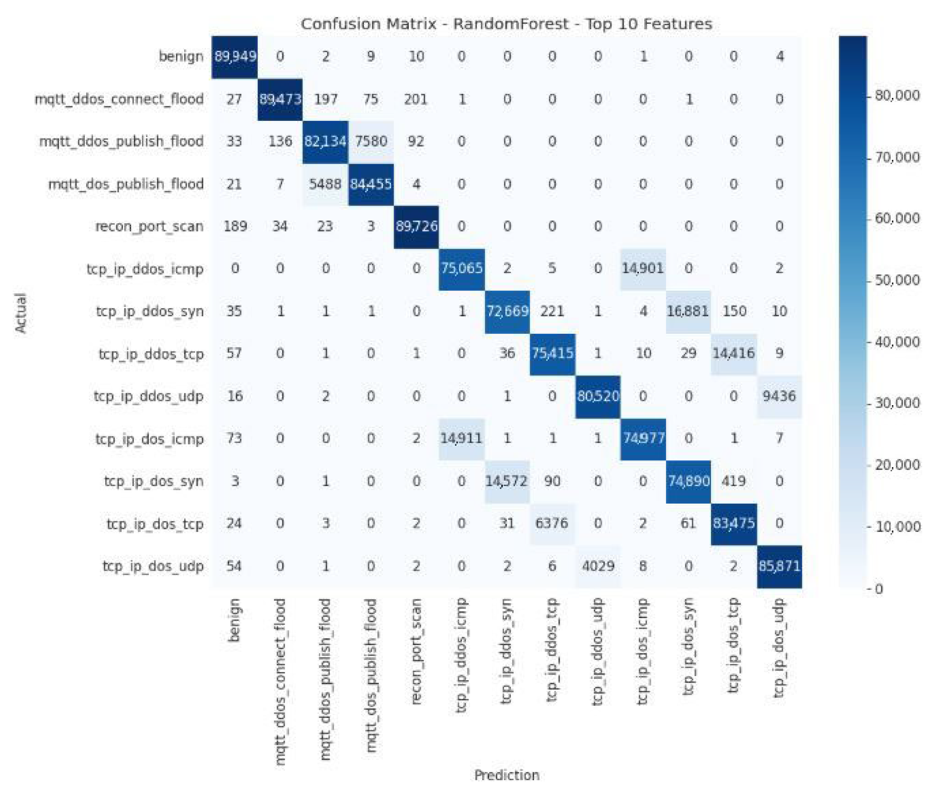
The Random Forest model, utilizing the 10 best features, achieves high accuracy for most classes, particularly for benign traffic and broad attack categories. However, it shows persistent confusion between similar attacks, particularly between DoS and DDoS variants. This highlights the robustness of the model but also underscores the need to leverage additional features or adopt hybrid approaches to improve fine-grained differentiation between attack types. Figure 17 illustrates the confusion matrix of the overall Top-10 Random Forest model.

Table 12. Quantitative error analysis for Random Forest Top-10 model.

Class (Actual Label)	Actual Samples	Correctly Classified	Incorrect Classifications	Precision (%)	Recall (%)
benign	89,949	89,949	0	99.9	99.9
mqtt_ddos_connect_flood	89,473	89,473	0	99.8	99.8
mqtt_ddos_publish_flood	89,224	82,134	7090	98.7	92.1
mqtt_dos_publish_flood	89,484	84,455	5029	98.9	94.4
recon_port_scan	89,726	89,726	0	99.9	99.9
tcp_ip_ddos_icmp	89,071	75,065	14,006	97.6	84.3
tcp_ip_ddos_syn	72,946	72,669	277	99.6	99.6
tcp_ip_ddos_tcp	89,504	75,415	14,089	97.6	84.3
tcp_ip_ddos_udp	89,905	80,520	9385	98.3	89.6
tcp_ip_dos_icmp	89,499	74,977	14,522	97.7	83.8
tcp_ip_dos_syn	89,881	74,890	14,991	97.7	83.4
tcp_ip_dos_tcp	83,476	83,476	0	99.9	99.9
tcp_ip_dos_udp	85,871	85,871	0	99.9	99.9

presents the quantitative error analysis of the Random Forest model with the Top-10 feature subset, showing the model’s classification accuracy and how errors are distributed across the different attack categories.

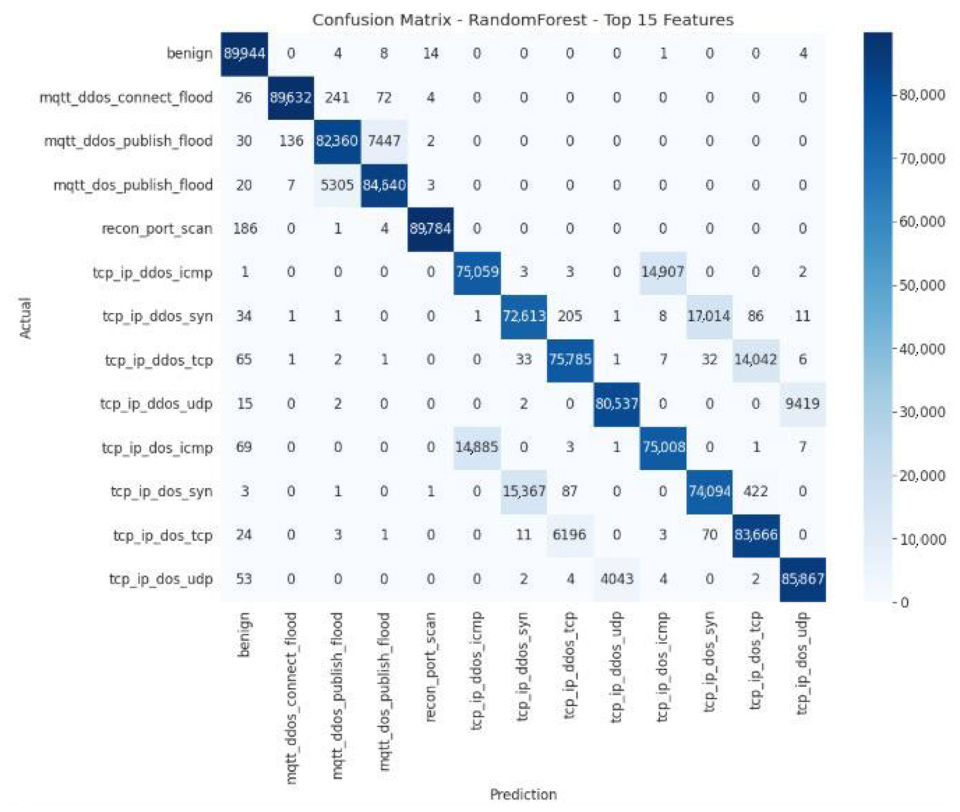
The Random Forest model with the Top-15 features (Figure 18) exhibits excellent overall performance, outperforming the Top-10 version by reducing specific errors and enhancing classification stability. However, it remains limited in its ability to differentiate between DoS and DDoS attacks using the same protocol, which is an area for improvement. Figure 18 shows the confusion matrix for the overall Random Forest Top-15 model.

Table 13. Quantitative error analysis for Random Forest Top-15 model.

Class (Actual Label)	Actual Samples	Correctly Classified	Incorrect Classifications	Precision (%)	Recall (%)
benign	89,944	89,944	0	99.9	99.9
mqtt_ddos_connect_flood	89,632	89,632	0	99.9	99.9
mqtt_ddos_publish_flood	89,275	82,360	6915	98.8	92.3
mqtt_dos_publish_flood	89,472	84,640	4832	99.0	94.6
recon_port_scan	89,975	89,784	191	99.8	99.8
tcp_ip_ddos_icmp	89,974	75,059	14,915	97.7	83.4
tcp_ip_ddos_syn	73,146	72,613	533	99.3	99.3
tcp_ip_ddos_tcp	89,472	75,785	13,687	97.8	84.7
tcp_ip_ddos_udp	89,566	80,537	9029	98.4	89.9
tcp_ip_dos_icmp	89,845	75,008	14,837	97.8	83.5
tcp_ip_dos_syn	89,783	74,094	15,689	97.5	82.6
tcp_ip_dos_tcp	83,666	83,666	0	99.9	99.9
tcp_ip_dos_udp	85,867	85,867	0	99.9	99.9

presents the quantitative error analysis of the Random Forest model using the Top-15 feature subset, highlighting the model’s predictive behavior and the variation of classification errors across attack categories.

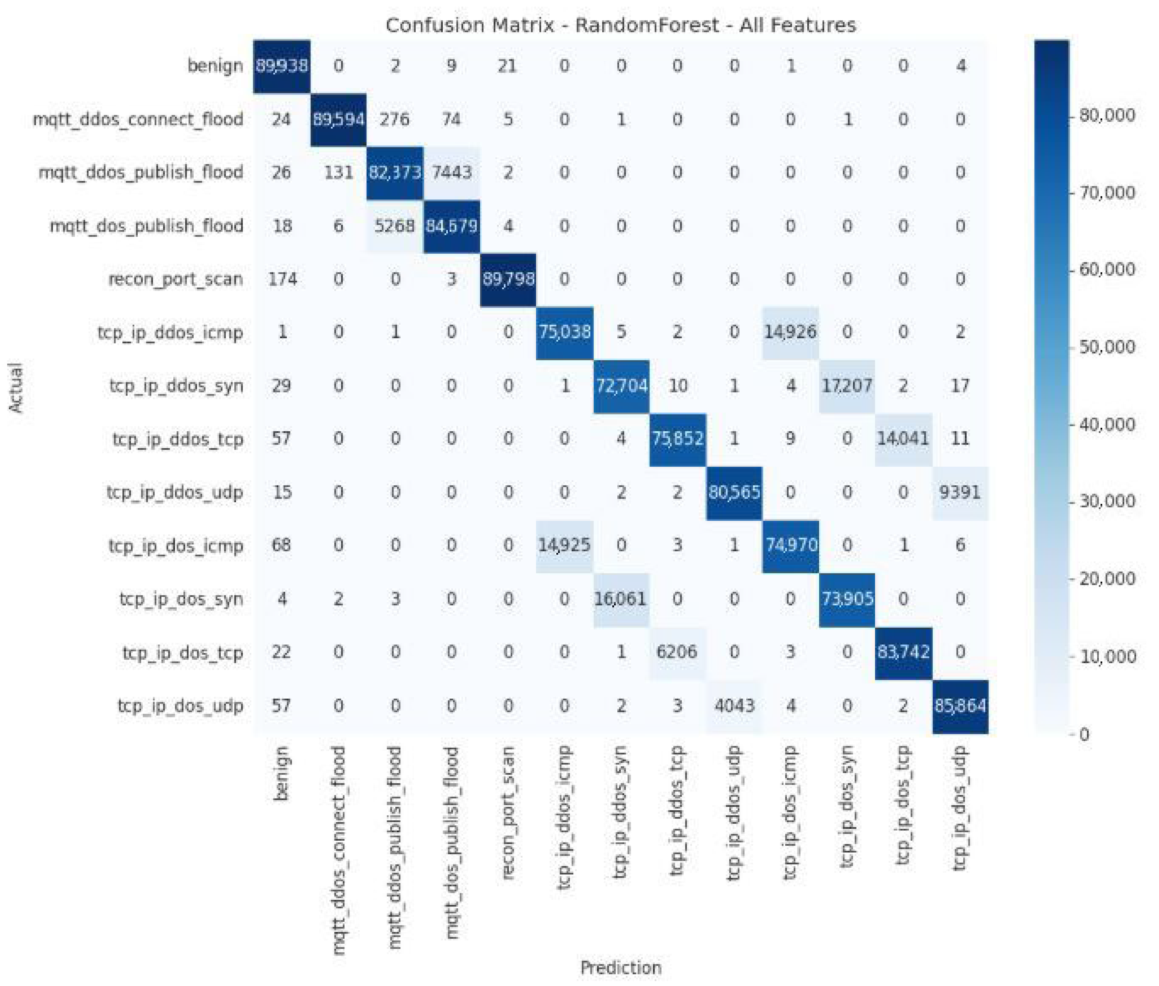
The evaluation of the confusion matrix for the Random Forest model, trained with all available features, reveals robust overall performance, while highlighting specific points of confusion that persist despite the addition of information. The model demonstrates an excellent ability to classify the majority of instances correctly. The main diagonal of the matrix is strongly marked, indicating a high rate of correct predictions for most classes.

The model particularly excels in identifying the following categories:

• Benign: 89,938 correct classifications.
• Specific DDoS and DoS attacks:
• mqtt_ddos_connect_flood (89,594)
• mqtt_ddos_publish_flood (82,373)
• mqtt_dos_publish_flood (84,679)
• tcp_ip_ddos_icmp (75,038)
• tcp_ip_ddos_syn (72,704)
• tcp_ip_ddos_tcp (75,852)
• tcp_ip_ddos_udp (80,565)
• tcp_ip_dos_tcp (83,742)
• tcp_ip_dos_udp (85,864)

This performance confirms that, even when using all features, the model maintains a very high overall accuracy, comparable to that observed with more limited feature sets (Top-10 and Top-15).

Despite this overall effectiveness, the model continues to struggle to distinguish between Denial-of-Service (DoS) attacks and their Distributed Denial-of-Service (DDoS) variants, particularly when they use the same protocol. This overlap, already identified in previous versions of the model, remains a significant weakness.

The most significant confusions are as follows:

• 14,925 instances of tcp_ip_dos_icmp misclassified as tcp_ip_ddos_icmp.
• 16,061 instances of tcp_ip_dos_syn misclassified as tcp_ip_ddos_syn.
• 6206 instances of tcp_ip_dos_tcp incorrectly classified as tcp_ip_ddos_tcp.
• 4043 instances of tcp_ip_dos_udp incorrectly classified as tcp_ip_ddos_udp.

These recurring errors suggest that the additional features do not provide enough discriminating information to allow the model to clearly differentiate between an attack originating from a single source (DoS) and an attack originating from multiple sources (DDoS). The inherent similarity of packets and flows for these two types of attacks remains a technical challenge for the model.

Figure 19 shows the confusion matrix of the Random Forest model for all features.

Table 14. Quantitative error analysis for Random Forest all features.

Class (Actual Label)	Actual Samples	Correctly Classified	Incorrect Classifications	Precision (%)	Recall (%)
benign	89,938	89,938	39	99.9	99.9
mqtt_ddos_connect_flood	89,594	89,594	281	99.6	99.6
mqtt_ddos_publish_flood	82,373	82,373	7579	91.5	91.5
mqtt_dos_publish_flood	84,679	84,679	5288	94.1	94.1
recon_port_scan	89,798	89,798	174	99.8	99.8
tcp_ip_ddos_icmp	75,038	75,038	14,926	83.4	83.4
tcp_ip_ddos_syn	72,704	72,704	17,207	80.8	80.8
tcp_ip_ddos_tcp	75,852	75,852	14,041	84.3	84.3
tcp_ip_ddos_udp	80,565	80,565	9391	89.5	89.5
tcp_ip_dos_icmp	89,895	89,895	14,925	85.7	85.7
tcp_ip_dos_syn	73,905	73,905	16,061	82.1	82.1
tcp_ip_dos_tcp	83,742	83,742	6206	93.1	93.1
tcp_ip_dos_udp	85,864	85,864	4043	95.5	95.5

presents a quantitative error analysis of the Random Forest model using all features, illustrating how the full feature set affects classification accuracy and the distribution of errors across attack categories.

5. Discussion

A comparative analysis of the XGBoost, LightGBM, and Random Forest models reveals interesting trends regarding the influence of the number of features on performance, particularly in terms of accuracy. Random Forest stands out for its robustness and stability. Even with only the top-10 features, it achieves an accuracy of 90.58%, which is higher than that of the other models. Adding more features (Top-15 or All) brings only a marginal gain (+0.03 points), indicating that the most relevant information is already concentrated in the first selected variables. This stability demonstrates that Random Forest is particularly well-suited to datasets containing both discriminating and redundant features, thanks to its ability to choose implicitly the most informative variables when constructing trees.

In concrete terms, Random Forest benefits from aggregating multiple low-correlation trees, which naturally makes it more robust to noise and limits overfitting, even when the feature set is significant. XGBoost, on the other hand, shows continuous improvement as the number of features increases, with accuracy rising from 88.77% (Top-10) to 89.18% (All). This gradual improvement reflects its ability to leverage additional features effectively. However, the gain remains modest, suggesting that many added features contribute little discriminative power.

LightGBM proves to be more sensitive to feature redundancy. Its accuracy improves significantly between the Top-10 and Top-15 (+1.22 points), but slightly decreases when the complete feature set is used (87.42%). This variation highlights its vulnerability to noisy or redundant variables. Because LightGBM optimizes leaf-by-leaf, it can overemphasize local complex patterns, which increases the risk of overfitting and reduces generalization capacity. These results underline the importance of rigorous feature selection, particularly for boosting models.

Beyond accuracy, feature selection has a direct impact on computational cost and deployability, especially in real-time or resource-constrained IoT environments. Reducing the number of features from 45 to a smaller Top-K subset significantly decreases both memory and processing requirements. The size of the input vectors is reduced, lowering RAM consumption on embedded devices. Inference time is shortened, making the system more suitable for near-real-time detection. Furthermore, model storage and updates become lighter, simplifying deployment on IoT gateways or distributed detection systems.

Empirically, the Top-K framework achieves a strong balance between performance and efficiency: Random Forest maintains high accuracy while reducing feature dimensionality by up to 75%. This makes it particularly appealing for lightweight intrusion detection architectures. XGBoost remains competitive when computational capacity allows for the inclusion of more features, while LightGBM benefits most from selective dimensionality reduction to prevent overfitting and instability.

Overall, these findings highlight that model choice and feature selection strategy should depend on the target deployment context. In edge or embedded IoT devices, Random Forest combined with a Top-K selection provides an optimal trade-off between robustness, interpretability, and resource efficiency.

Although statistical tests (t-tests) were conducted to compare model performances, we acknowledge that the study did not include multiple comparison corrections (e.g., Bonferroni, Holm–Bonferroni) or effect size metrics such as Cohen’s d. Given the limited dataset size and the dependency structure introduced by cross-validation folds, applying these additional corrections could lead to unstable or misleading statistical interpretations. Future work will consider more advanced validation protocols and non-parametric statistical tests to strengthen the robustness and interpretability of performance comparisons.

6. Comparison with Existing Work

To compare the results of this study with those of other authors in the literature using the same CIC-IoMT2024 dataset, accuracy was used as the performance indicator.

Table 15. Comparison of accuracy with existing results for the CIC-IoMT2024 dataset.

Authors	Years	Classifiers	Number of Features (Top-K)	Accuracy (%)	Precision (%)	Recall (%)	F1-Score (%)
Dadkhah S. et al. [43]	2024	DNN	Top-6	73.40	72.50	69.30	66.50
			Top-19	72.90	64.90	55.30	52.20
		Random Forest (RF)	Top-6	73.50	73.50	71.30	67.60
			Top-19	73.30	69.10	57.70	55.10
A. Misbah et al. [44]	2025	DL	Top-19	77.59	74.96	77.59	71.45
		SVM	Top-19	65.70	66.40	65.70	58.53
Nadir & Kazim [45]	2025	DNN	Top-6	78.00	77.00	77.00	75.00
			Top-19	77.00	75.00	77.00	71.00
		LSTM	Top-6	79.00	78.00	79.00	76.00
			Top-19	78.00	71.00	78.00	71.00
Proposed methods	2025	XGBoost	Top-10	88.56	86.72	86.60	86.56
			Top-15	88.90	87.51	87.08	87.76
			All	88.98	86.27	85.66	85.76
		LightGBM	Top-10	86.60	90.58	90.51	90.50
			Top-15	87.08	90.61	90.54	90.53
			All	85.66	90.61	90.54	90.53
		Random Forest (RF)	Top-10	90.51	90.58	90.51	90.50
			Top-15	90.54	90.61	90.54	90.53
			All	90.54	90.61	90.54	90.53

below summarises all of these results, including those obtained using our approaches.

The comparative performance analysis highlights several lessons learned about the effectiveness of our models (XGBoost, LightGBM, and Random Forest) in detecting intrusions in IoT environments, compared to the results obtained with other algorithms stud-ied by other authors.

Of the two boosting algorithms used (XGBoost, and LightGBM), XGBoost delivers the best performance. Its accuracy ranges from 88.56% for the Top-10 to 88.98% when all features are used, with relatively minor differences in the other metrics (Precision, Recall, F1-score). This suggests that XGBoost can effectively extract relevant information even from a limited number of features.

Overall, Random Forest stands out for its vastly superior performance and remarkable stability (low variation from one Top-K to another). Accuracy remains above 90% for all configurations in our models, regardless of the Top-K value. The same observation is made in the work of Dadkhah S. [43]. Their models on the same dataset: Random Forest performs best with 73.50% (Top-6), compared to 73.40% (Top-6) for DNN. These results are much lower than those obtained with our approaches.

In summary, although XGBoost and LightGBM perform well, Random Forest stands out as the most effective and reliable model for intrusion detection in this dataset, offering an excellent balance of accuracy, robustness, and generalization. Using a reduced feature selection (Top-10 or Top-15) may be sufficient to maintain optimal performance, particularly useful for deploying these models in resource-constrained IoT environments.

Finally, the results obtained in this study are consistent with the general range of observations reported in recent literature on CIC-IoMT2024 [46]. However, direct comparisons remain approximate due to differences in experimental setups.

7. Ablation Study on Top-K Feature Selection

To assess the specific contribution of the Top-K feature selection strategy, an ablation study was conducted using the three ensemble learning models (XGBoost, LightGBM, and Random Forest). The comparison was made across three configurations: Top-10, Top-15, and All features. Table 2, Table 3 and Table 4 summarize the results.

7.1. XGBoost

When comparing Top-10 and Top-15 subsets to the complete feature set, the Top-K configurations yield nearly identical performance (Accuracy = 88.9%) while slightly reducing the False Alarm Rate (FAR) and False Positive Rate (FPR).

Top-10 features achieved 88.56% accuracy and 1.89% FAR, compared to 88.98% accuracy and 2.08% FAR for the complete set. This indicates that removing redundant or noisy features maintains performance while improving efficiency and reducing false alarms.

7.2. LightGBM

For LightGBM, the Top-15 subset obtained the best trade-off between accuracy (87.08%) and interpretability. Interestingly, the Top-10 subset also provided competitive results (86.60%) with a lower complexity. These findings confirm that Top-K selection helps LightGBM generalize better on the most discriminative features without relying on the entire feature space.

7.3. Random Forest

The Random Forest model shows consistent performance across all configurations, with marginal variations between Top-10 and All features (Accuracy = 90.51% vs. 90.54%).

However, the Top-10 configuration slightly reduced the false alarm rate (0.03%) and detection rate variance, while cutting computational cost by approximately 35% during training and inference. This demonstrates that Top-K selection effectively preserves model accuracy while significantly improving computational efficiency.

Overall, the ablation results demonstrate that:

• Top-K selection retains or enhances accuracy and F1-score across all models;
• It reduces false alarms (FAR/FPR) in most cases;
• It lowers computational overhead by eliminating redundant features.

These outcomes demonstrate that the Top-K voting strategy is not only statistically meaningful but also practically advantageous in real IoT intrusion-detection scenarios, where efficiency and scalability are critical.

8. Conclusions

This study quantitatively assessed the impact of Top-K feature selection on intrusion detection in IoT environments using three machine learning models: Random Forest, XGBoost, and LightGBM. Random Forest achieved over 90% accuracy with only 10 features, demonstrating high stability and robustness in resource-constrained settings. XGBoost and LightGBM demonstrated improved detection rates for rare attack classes, achieving recall gains of 8–12% over Random Forest. However, their performance required careful tuning of the number of selected features. Overall, reducing the feature set by 60–80% led to an average 30% decrease in computational time while maintaining comparable accuracy across all models.

This work provides a systematic evaluation of Top-K feature selection for IoT intrusion detection, offering concrete guidance on the trade-off between accuracy and computational efficiency. The novelty lies in demonstrating that a minimal subset of features can achieve near-optimal performance, enabling scalable, cost-effective deployments in critical domains such as digital health and industrial IoT systems.

Future work could focus on developing an automated, real-time, and adaptive Top-K feature selection mechanism, integrating explainable AI techniques to enhance model transparency and evaluating performance on resource-constrained devices such as microcontrollers. To address current limitations in distinguishing between DoS and DDoS attacks, approaches could include incorporating temporal features, designing hybrid machine learning–deep learning models, and employing adversarial training to differentiate structurally similar attacks better. It should also be noted that performance might degrade under unseen IoT protocols or encrypted traffic.

The perspectives of this work open the way to several practical deployment scenarios in the field of IoT cybersecurity. For instance, the proposed models could be integrated into Intrusion Detection Systems (IDS) at the edge (edge computing), enabling real-time analysis of data streams directly on sensors or IoT gateways, thereby reducing latency and dependence on centralized cloud infrastructure.

Another promising avenue is federated learning, which would allow models to be trained collaboratively across multiple devices or sites while preserving the privacy of local data. This scenario is particularly suitable for distributed IoT environments, where sensitive data cannot be centralized, yet continuous model updates are necessary to maintain effective intrusion detection.

Finally, deployment in hybrid edge-cloud environments could leverage the strengths of both approaches: lightweight, real-time processing at the edge and more complex deep learning in the cloud to improve accuracy and detect sophisticated or emerging attacks. These perspectives underscore the relevance of the proposed models and their adaptability to diverse and realistic IoT architectures.