Article

Scalable Generation of Synthetic IoT Network Datasets: A Case Study with Cooja

by
Hrant Khachatrian
1,2,
Aram Dovlatyan
2,
Greta Grigoryan
1 and
Theofanis P. Raptis
3,*
1
Machine Learning Group, Center for Mathematical and Applied Research, Yerevan State University, Yerevan 0025, Armenia
2
YerevaNN, Yerevan 0025, Armenia
3
Institute of Informatics and Telematics, National Research Council, 56124 Pisa, Italy
*
Author to whom correspondence should be addressed.
Future Internet 2025, 17(11), 518; https://doi.org/10.3390/fi17110518 (registering DOI)
Submission received: 21 October 2025 / Revised: 5 November 2025 / Accepted: 11 November 2025 / Published: 13 November 2025

Abstract

Predicting the behavior of Internet of Things (IoT) networks under irregular topologies and heterogeneous battery conditions remains a significant challenge. Simulation tools can capture these effects but can require high manual effort and computational capacity, motivating the use of machine learning surrogates. This work introduces an automated pipeline for generating large-scale IoT network datasets by bringing together the Contiki-NG firmware, parameterized topology generation, and Slurm-based orchestration of Cooja simulations. The system supports a variety of network structures, scalable node counts, randomized battery allocations, and routing protocols to reproduce diverse failure modes. As a case study, we conduct over 10,000 Cooja simulations with 15–75 battery-powered motes arranged in sparse grid topologies and operating the RPL routing protocol, consuming 1300 CPU-hours in total. The simulations capture realistic failure modes, including unjoined nodes despite physical connectivity and cascading disconnects caused by battery depletion. The resulting graph-structured datasets are used for two prediction tasks: (1) estimating the last successful message delivery time for each node and (2) predicting network-wide spatial coverage. Graph neural network models trained on these datasets outperform baseline regression models and topology-aware heuristics while evaluating substantially faster than full simulations. The proposed framework provides a reproducible foundation for data-driven analysis of energy-limited IoT networks.

1. Introduction

1.1. Background

The proliferation of Internet of Things (IoT) applications has intensified the need for rigorous testing and validation of wireless sensor networks operating under resource constraints [1]. Low-power wide-area networks, particularly those based on the IPv6 Routing Protocol for Low-Power and Lossy Networks (RPL), must maintain connectivity and coverage despite irregular topologies, constrained energy budgets, and unpredictable node failures [2]. Understanding network behavior under these conditions typically requires extensive simulation campaigns [3], as physical deployment of hundreds of battery-powered devices across diverse topologies remains prohibitively expensive and impractical for systematic design-space exploration [4].
Cooja [5], an extensible network simulator integrated with Contiki-NG [6], provides a powerful environment for emulating IoT networks by executing actual firmware binaries. However, coordinating large-scale simulation campaigns containing thousands of runs with varying topologies, battery configurations, and protocol parameters demands significant manual labor and configurations. Each simulation requires careful preparation of network topology descriptions, firmware compilation, parameter specification, and post-processing of voluminous log outputs [7]. This manual workflow becomes impractical when generating datasets sufficiently large and diverse for training predictive models [8]. To automate such large campaigns, Cooja can be executed in, where simulations run without the graphical UI and are controlled from the command line. Headless execution enables scripted/programmatic and non-interactive batch runs on servers or compute clusters.
Recent advances in graph neural networks (GNNs [9]) have shown an exceptional capability in learning from network-structured data, suggesting that surrogate models could approximate simulation outcomes at orders of magnitude lower computational cost [10]. Such approximations enable rapid what-if analysis during network design [11]: designers could iteratively explore configurations that may include actions like adjusting node densities, battery capacities, or deployment geometries and receive near-instantaneous predictions of coverage, connectivity duration, and failure modes without invoking the simulator for each variant [12].

1.2. Our Contribution

This paper presents an end-to-end pipeline for automated generation and analysis of large-scale IoT network datasets. Our framework integrates parameterized topology generators with Slurm-orchestrated Cooja simulation sweeps, enabling synthesis of richly annotated datasets capturing complex network dynamics. We demonstrate the framework through a comprehensive case study on RPL networks, generating over 10,000 simulations with irregular sparse-grid topologies, randomized battery allocations, and node populations ranging from 15 to 75 motes. The resulting dataset captures phenomena challenging classical analytical models: nodes that fail to establish routes despite physical connectivity, cascading failures triggered by relay battery depletion, and spatially heterogeneous coverage degradation.
Using this dataset, we train graph neural network models to predict two critical network metrics: per-node time of last successful message delivery to the root (indicating when individual nodes lose contact with the network) and network-wide spatial coverage assuming a 30 m sensing radius per active node. Our GNN architecture leverages the natural graph structure of communication networks, embedding spatial coordinates, battery states, and radio-range-based connectivity into learned representations. These models significantly outperform baseline predictors, including linear regression on battery features and topology-aware heuristics, while enabling inference several orders of magnitude faster than simulation, facilitating rapid design iteration and reliability analysis.
Our work addresses two complementary challenges in large-scale IoT network analysis. The first challenge concerns dataset generation. Exploring the behavior of routing protocols such as RPL under diverse conditions requires thousands of network simulations. Running such experiments manually is both inefficient and difficult to reproduce. To address this, we develop an automated pipeline that generates diverse network topologies, configures and executes headless Cooja simulations, and extracts structured outputs from simulation logs while managing execution across distributed compute nodes. The second challenge is efficient prediction of network behavior. Once datasets are available, we aim to build surrogate models that approximate key simulation outcomes at much lower computational cost. Given a network configuration that is defined by node positions, initial battery levels, and connectivity, we predict (i) the time at which each non-root node last successfully communicates with the sink before failure and (ii) the overall sensing coverage area of active nodes. These models enable rapid what-if analysis and large-scale reliability studies that would be infeasible with full simulations.

1.3. Related Work and Novelty

Prior research on IoT network simulation and analysis has largely focused on improving fidelity or scalability within specific simulation tools rather than automating the entire experimentation process [13,14]. Frameworks such as IoTSim-Edge [15] and iFogSim2 [16] enable modeling of large-scale IoT–edge–cloud systems, but they typically operate at the level of abstract workload flows and virtualized resources rather than executing actual low-power firmware. Conversely, simulators based on Contiki or TinyOS, such as Cooja [5] and TOSSIM [17], achieve high fidelity by running native embedded code but require significant manual configuration to produce diverse, reproducible experiments. Recent efforts have introduced scripting interfaces to simplify Cooja-based campaigns [7], yet these approaches remain limited to static experiment templates and lack end-to-end orchestration across distributed computing infrastructures.
Our work advances the state of the art in two fundamental ways. First, it introduces a fully automated, Slurm-orchestrated pipeline for large-scale, reproducible simulation campaigns using Cooja. Unlike prior scripting or GUI-assisted approaches, our framework automatically generates parameterized topologies, compiles and executes thousands of firmware instances, and extracts structured outputs for downstream analysis, enabling the creation of datasets orders of magnitude larger and more diverse than in existing literature. This constitutes, to our knowledge, the first publicly documented workflow that scales Cooja-based RPL simulations to tens of thousands of runs with heterogeneous spatial and energy configurations. Second, we demonstrate that graph neural networks can accurately learn surrogate models of RPL network behavior directly from these large-scale simulation datasets. Our GNNs predict per-node disconnection times and network-wide sensing coverage with significantly higher accuracy than baseline analytical or regression models while reducing inference time by several orders of magnitude compared to full simulations. This integration of automated dataset generation and graph-based surrogate modeling establishes a novel methodology for rapid what-if analysis and reliability assessment of IoT networks, a capability not addressed in prior works on either simulation automation or learning-based network prediction.

2. Methodology

2.1. Simulation Environment

We conduct our experiments using Cooja, the network simulator bundled with Contiki-NG that enables cycle-accurate emulation of IoT firmware. Unlike typical simulation studies that rely on Cooja’s graphical interface for manual configuration, we operate entirely in headless mode (no GUI), which enables programmatic control and parallel execution across computational resources. This approach extends what is typically an interactive tool into a scalable data generation engine.

2.2. Automation Pipeline

Figure 1 summarizes the staged flow from experiment specification to structured data products. The framework executes five stages with persisted artifacts at each boundary: topology JSON → CSC → Cooja log → parsed CSV. There is also an option to insert the contents of the parsed CSVs into specified PostgreSQL database table(s). Our framework orchestrates the complete workflow from topology specification to structured dataset creation through a series of modular stages. The pipeline operates as follows:
  • Stage 1: Topology specification.
A parameterized topology generator produces network layouts encoded in JSON, specifying node positions, roles (sink/server versus source/client), and connectivity constraints. The generator supports multiple topology categories, including regular grids, trees, random meshes, and sparse irregular grids. Each topology undergoes validation to ensure graph connectivity and the feasibility of the radio range. We ensure that a topology is a single connected component so that at the start of simulations, all motes can reach the server/sink. Additional constraints and validations for topologies can be added as desired. For our case study, we generate sparse grids with controlled position jitter, creating realistic deployments where nodes typically maintain 2 to 6 neighbors.
  • Stage 2: Simulation configuration.
A CSC generator creates the sim.csc file from the topology JSON. The configuration binds prebuilt firmware to motes, sets UDGM parameters (transmit and interference ranges), places motes at the specified coordinates, and defines the simulation duration. A ScriptRunner plugin that allows you to execute JavaScript code during the headless Cooja runs standardizes log records by attaching timestamps, mote IDs, and a run identifier, which makes per-line parsing deterministic across large sweeps. The only way to get access to logs when running headless Cooja is to include the ScriptRunner plugin and code that logs events in the simulations.
  • Stage 3: Execution.
Headless Cooja executes one run per configuration in an isolated working directory and writes a consolidated cooja.log. A batch orchestrator schedules array jobs, constrains resources, and retries failed runs. Auxiliary console output (toolchain and simulator messages) is captured in stdout.txt for diagnostics.
  • Stage 4: Parsing.
A parser processes cooja.log and emits tabular outputs: results.csv (per-node/per-event records) and results_xy.csv (records joined with coordinates). Run-level context is preserved in run_meta.json and role mappings in roles.json. Pattern matching targets well-formed tags from firmware and ScriptRunner (e.g., deliveries to the sink, route changes, battery updates), and computes derived quantities such as time of last successful delivery.
  • Stage 5: Dataset assembly.
Per-run CSVs are merged into experiment-level tables with consistent column schemas. Optional loaders materialize the dataset into a relational database to support scalable queries and model training pipelines.
  • Customization and extensibility.
The pipeline defines a compact set of required inputs and optional extension points that control experiment composition and output integration. Required components are (1) mote firmware for the sink and sensing motes (src/*.c), (2) the topology family with its associated parameter ranges, and (3) the sweep configuration specifying simulation duration, random seeds, radio parameters, and battery distributions. Optional components extend the workflow with custom parsers aligned to firmware message schemas, dataset builders that assemble ML-ready tables, and database loaders for persistent storage or remote querying. Table 1 enumerates these components and their roles in the automation workflow.
  • Intermediate artifacts.
Each simulation produces a structured set of outputs stored in a dedicated directory. Typical files include topology.json, the generated sim.csc configuration, the raw cooja.log, parsed CSV outputs (results.csv, results_xy.csv), and metadata files (roles.json, run_meta.json). Auxiliary outputs such as stdout.txt are preserved. These artifacts collectively capture the full provenance of each simulation run and facilitate downstream aggregation or database ingestion.

2.3. Steps to Design the Experiment Pipeline

This modular architecture ensures extensibility: new topology generators, firmware variants, custom mote implementations, or derived metrics can be integrated without making changes to the core orchestration logic. The framework has successfully generated datasets exceeding 10,000 simulations, each producing multi-megabyte log files, which demonstrates configurability, robustness, and scalability.
Here are the steps that a practitioner designing a large-scale simulation should perform to leverage the framework:
  • Implement the motes/firmware. In practice, these are .c files that Contiki-NG can execute. These files also define what is going to be logged in each simulation.
  • Choose the topology or define a new one.
  • Define the ranges of simulation configurations, i.e., the number of motes, transmission and interference ranges, and random seed.
  • Implement the parser for the logs generated during the simulations.
  • Implement a dataset aggregator, i.e., a script that scans the parsed logs of all simulations and produces an ML-ready dataset, typically a CSV file with inputs and outputs, possibly with additional references to simulation-specific outputs.

2.4. Case Study: RPL Network Analysis

We demonstrate the framework’s capabilities through a comprehensive study of RPL networks operating under battery constraints and irregular topologies. The RPL protocol was chosen as the target protocol due to its widespread adoption in IoT research and its native support within the Contiki-NG and Cooja simulation environments. RPL is known to exhibit non-trivial behaviors under heterogeneous battery conditions and irregular topologies, including unstable parent selection, persistent unjoined nodes, and cascading link failures resulting from energy depletion. These phenomena make RPL an ideal testbed for assessing the ability of machine learning models to predict node- and network-level performance degradation in energy-constrained IoT deployments.
High-level scenario description: We simulate wireless sensor networks where each node is positioned across a pre-defined grid (with some noise) on a 2D plane, collects some data, and sends it to the designated root node that acts as a sink and is always located at (0, 0) coordinates. The setup corresponds to a scenario where several dozen nodes are thrown over a field; each node senses its immediate neighborhood on the field and reports the data to the root node on the edge of the field at regular time intervals. We note that the root node is fixed at the coordinate (0, 0), following a common convention in IoT simulations where the sink or gateway is placed at the edge or corner of the monitored region to emulate realistic data collection scenarios. This design choice does not introduce topological bias for the GNN models, as the relative spatial relationships among nodes are preserved under translation or rotation of the network layout. Equivalent configurations with the root placed in other corners (e.g., (0, N), (N, 0), or (N, N)) would yield identical graph connectivity patterns up to coordinate transformations, thus not affecting model generalization. The nodes have random battery capacities at the start of the simulation and might go offline at some point in the simulation due to battery depletion. The connectivity is implemented using the RPL protocol, which causes uneven CPU usage across the nodes as some nodes forward more messages than others.
Once one of the nodes turns off, the traffic is redirected through other nodes, which causes more uneven and less predictable CPU utilization, hence less predictable node lifetime. Messages from node i stop reaching the root node, not only when the node itself goes offline, but also when the network loses connectivity due to intermediate nodes (between i and the root node) going offline. Due to these factors, it is quite challenging to predict how long the root node will receive messages from each of the other nodes. Hence, machine learning methods trained on a large dataset of simulations can be useful.
Another important challenge is to understand the actual area covered by the sensor network. Each node senses its neighborhood with a pre-defined radius, but due to RPL complexities and interference, not every node will join the network before some of the nodes go offline. We call this the coverage prediction problem and frame it as another machine learning task.
1. Implementing motes: We utilized Zolertia Z1 motes, which run standard Contiki-NG firmware with RPL routing. We specifically selected the Z1 platform, as it supports the emulation of low-power mode (LPM) of CPUs. In this case, the nodes that send or forward more messages will utilize significantly more CPU power (vs. LPM), and the battery will drain faster.
We have implemented two types of motes, server and client, based on the UDP-RPL examples in the official Contiki-NG repository [6]. Nodes employ Contiki-NG’s implementation of the RPL protocol with default Objective Function Zero (OF0) for route selection.
We have integrated the Energest [18] module to track energy usage based on CPU and radio activity. Energest tracks the time of each component, and we use the following formula (inspired by [19]) to calculate the energy usage:
E t = 1.8 * CPU + 0.0545 LPM + 20.0 RadioRx + 17.4 RadioTx
Each node has an initial energy E 0 , which is uniformly sampled between 25 and 100 mAh. Once the energy usage exceeds the initial energy ( E t E 0 ), the node powers off. Each node sends a message to the root every 5 s before it goes offline.
We have implemented comprehensive logging to capture per-node events, including route establishment, message transmissions, battery state, and failure timestamps. This is configurable, and you may set the logging level in project-conf.h to control logging granularity for Cooja simulations.
2. Defining the topology: We place nodes on a coarse grid and add a small random spatial jitter to each position to avoid unrealistic regularity and better reflect practical deployments. Given the number of nodes N and grid spacing S, we
(i)
draw grid dimensions by sampling R , C Unif { N , , 1.5 N } and instantiate an R × C grid with spacing S;
(ii)
put the root node at ( 0 , 0 ) ;
(iii)
sample N 1 distinct grid sites without replacement for non-root nodes;
(iv)
add independent jitter to each non-root node: ( Δ x , Δ y ) Unif [ S / 2 , S / 2 ] 2 ;
(v)
check connectivity under a 50 m communication radius by forming the proximity graph (edges between nodes within 50 m) and verifying that all nodes are reachable from the root; if not, we start back from Step (i) by resampling the grid and jitter. We repeat this loop up to 10 times. In practice, the algorithm always found a connected graph within one to five attempts.
In real deployments, node placement is never perfectly uniform because equipment is attached to walls, poles, or trees, or positioned manually with small errors. Adding spatial jitter models to this variability while preserving overall node density leads to more realistic neighbor distances and routing behavior.
3. Configuring simulations: Each simulation executes for 300 s of simulated time with millisecond-resolution timestamping. Radio communication follows the Unit Disk Graph Medium (UDGM) model with a 50-m transmission range, a 100-m interference range, and a success ratio of 1.0 for both transmission and reception.
We generate topologies with N [ 15 , 75 ] nodes. For each value of N, we vary spacing S { 20 , 22 , , 30 } (in meters) and the random seed from 1 to 30. This would result in 61 · 6 · 30 = 10,980 simulations. Before running the main grid of simulations, we had an initial test run that simulated 52 topologies ( 34 N 49 , S = 20 ) that we decided to keep in the final dataset, resulting in 11,032 networks.
4. Implementing the log parser: Cooja simulation stores the logs produced by all the motes in a single large log file. Due to highly granular logging, the log files are a few megabytes in size. We have implemented a parser that reads the log file and produces a CSV with one row for each mote and the following columns: x and y coordinates of the mote (which is extracted from the topology file), initial battery level, all Energest values (total time spent in CPU, LPM, RadioRx, and RadioTx modes during the entire course of the simulation), the amount of energy consumed, status of the mote (alive or dead), uptime, number of messages sent and forwarded, and the time the last message was received by the root node. Note that the latter is set to −1 when no messages were received from the node. Table 2 shows a typical example.
5. Implementing dataset aggregation: We wrote a basic Python 3.11 script to aggregate all processed CSVs from the previous steps into a single CSV that describes the whole dataset. Each row describes one simulation and has the following columns: number of motes N, spacing S, random seed, Slurm job ID (for debugging), split, coverage, and number of active nodes during the simulation. The coverage is calculated by drawing circles with a 30 m radius centered on each node that has sent at least one message to the root node and measuring the total area of the circles.
Dataset composition: We generated 11,032 distinct simulations spanning diverse network sizes and spatial configurations. Each run produces structured data comprising per-node initial conditions (coordinates, battery capacity), temporal event logs (route formation, message delivery, disconnection), and summary statistics (network lifetime, coverage decay, per-node uptime). The dataset exhibits rich variability: some networks maintain full connectivity throughout the simulation despite battery heterogeneity, while others experience rapid fragmentation due to relay placement or extreme battery imbalances. We randomly split the dataset into training, validation, and test sets.

2.5. Baselines

To contextualize GNN performance, we evaluate two baseline predictors for each of the tasks.
Contact loss prediction baselines based on training set statistics: The first baseline is the Mean Predictor, which simply groups the nodes by their initial battery level and predicts the training-set mean over the group based on the initial energy. This baseline provides a reference for assessing whether learned models capture any meaningful structure beyond simple statistics.
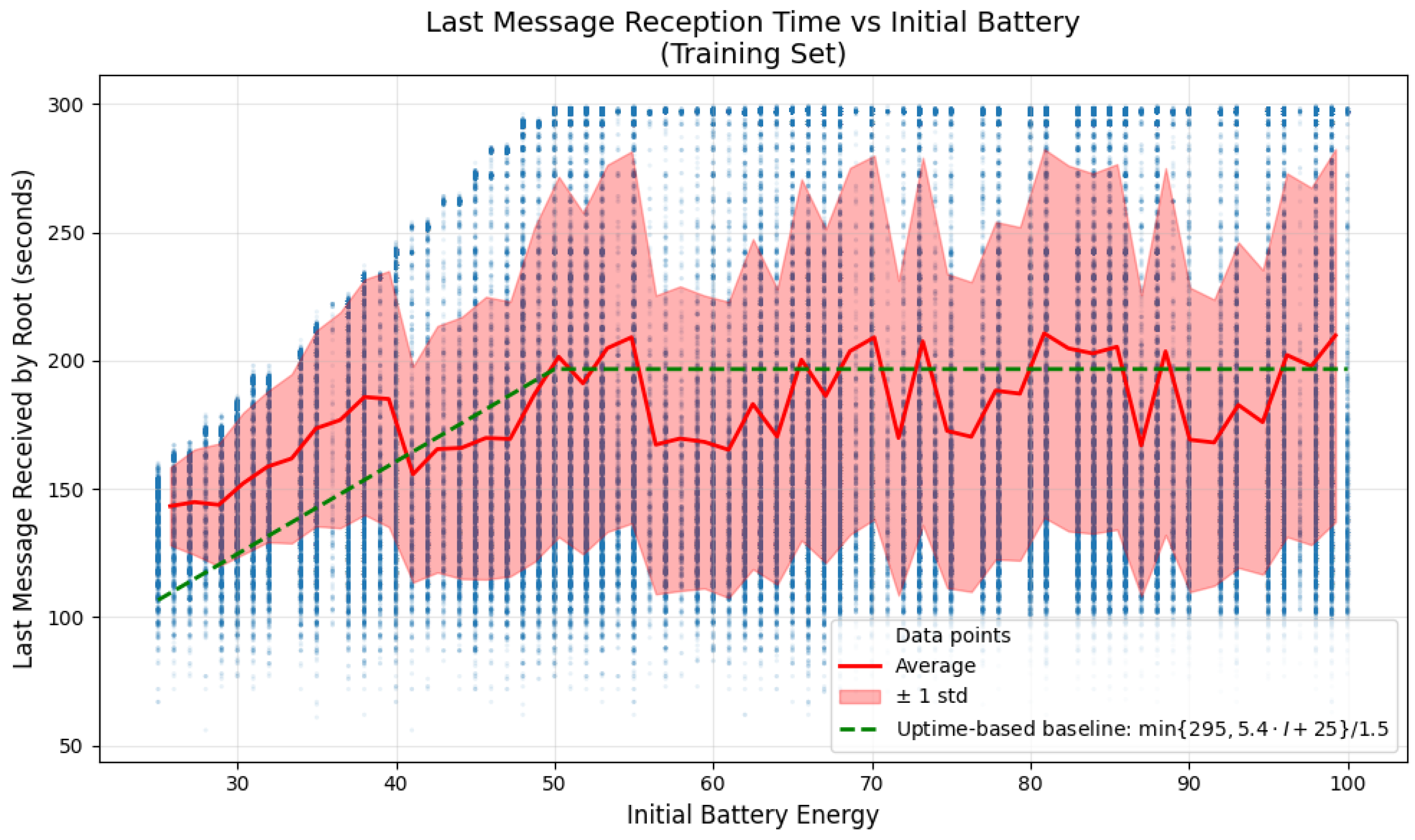
The second baseline is the Uptime-Based Predictor. This approach models contact loss as a piecewise linear function of the initial battery capacity. Analysis of the dataset shows that the uptime of each node is basically a linear function of the initial battery power (I), capped at the simulation time. The coefficients for the linear function were fitted to the data, resulting in the following near-accurate formula for uptime:
U = min { 295 , 5.4 · I + 25 }
Contact loss is usually less than the uptime due to the power loss on the intermediate nodes. Hence, this formula can be scaled to provide a more accurate prediction for contact loss. We take U 1.5 as a baseline. Note that this baseline captures first-order energy effects but ignores spatial structure.
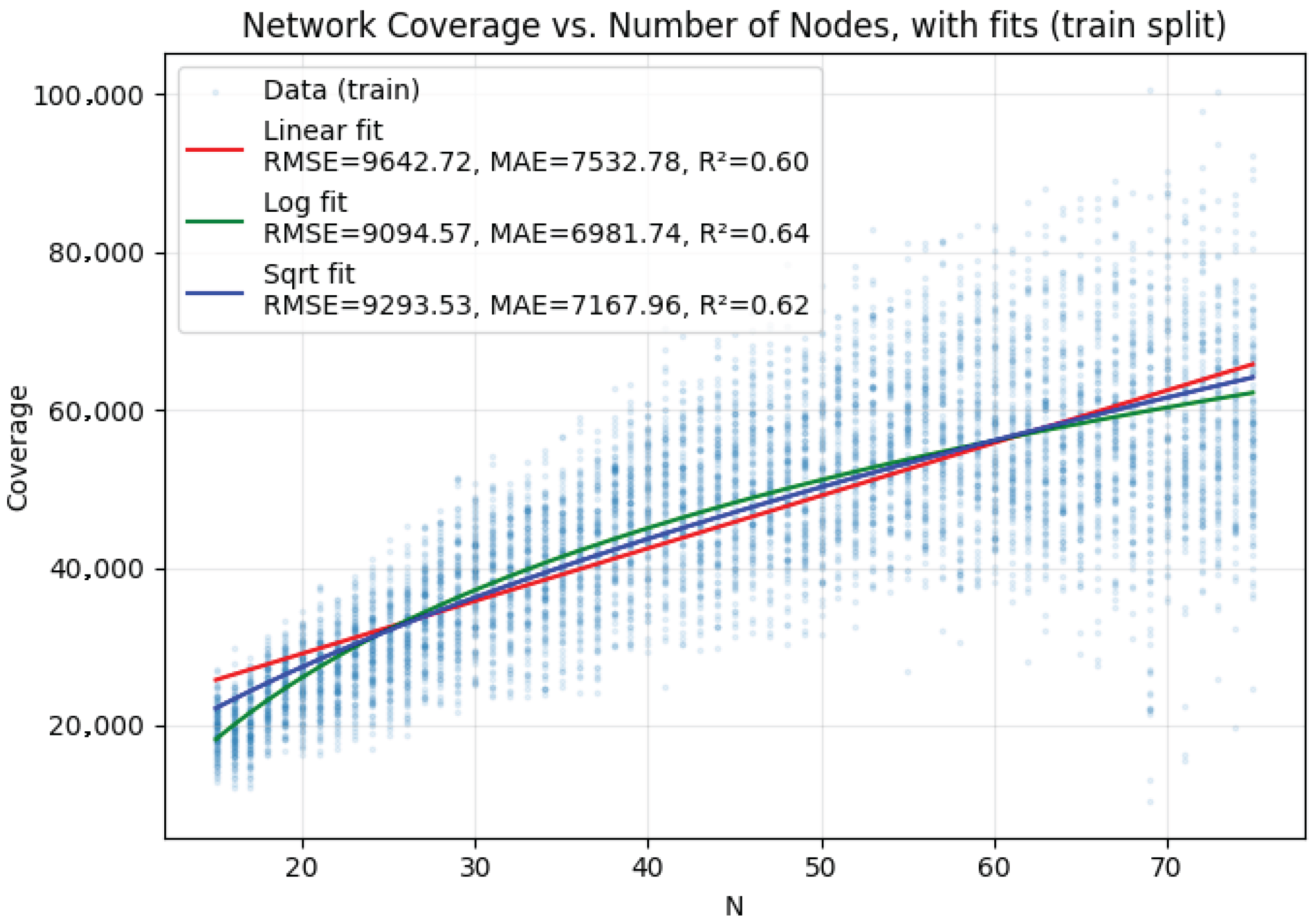
Topology-aware baselines for coverage prediction: The first baseline for coverage prediction is implemented by fitting the coverage with respect to log ( N ) over the training set, where N is the number of nodes. We also tried N and N, but the logarithm worked better.
The second baseline is geometric; it leverages the coordinates of the nodes. We draw (overlapping) circles with a 30 m radius centered on the node locations on a plane (using OpenCV) and calculate the total area covered. We note that some nodes, especially those with low initial battery, might not be able to send any message before they go offline, so we discard the circles around nodes with an initial battery less than some threshold B. We tuned B and found B = 50 to be optimal.
All baselines are trained on the same training split and evaluated on the independent test set, ensuring a fair comparison.

2.6. Graph Neural Networks for Predicting Network Behavior

We formulate network behavior prediction as supervised learning on attributed graphs. Each simulation is represented as a graph G = ( V , E , X ) where vertices V correspond to network nodes, edges E V × V represent communication feasibility (nodes within 50-m radio range), and node attributes X R | V | × d encode initial conditions (spatial coordinates, battery capacity).
Architecture: Our GNN employs GraphSAGE [20] convolutional layers, which aggregate information from local neighborhoods through learnable transformations. The network comprises the following:
  • Node encoder: A two-layer multi-layer perceptron maps raw node features (x-coordinate, y-coordinate, initial battery) to an H-dimensional embedding space. Features are normalized using training set statistics to ensure balanced gradient magnitudes.
  • Graph convolutions: L GraphSAGE layers progressively refine node embeddings by aggregating information from expanding neighborhoods. Each layer applies a mean aggregation over neighbor embeddings, followed by a learned linear transformation and ReLU activation. More advanced aggregation methods can potentially improve the performance, but we left this exploration for future work. Residual connections and layer normalization stabilize training on deep architectures.
  • Task-specific predictors: For node-level prediction (contact loss), a two-layer MLP maps refined node embeddings to scalar outputs. For graph-level prediction (coverage), node embeddings are aggregated via global mean pooling, concatenated with graph-level features (node count, grid spacing), and passed through a prediction MLP.
Edge construction: The communication graph is constructed by connecting nodes within 50 m (the radio transmission range), mirroring the Unit Disk Graph connectivity model used in simulation. Edge attributes encode Euclidean distance between connected nodes, providing the GNN with explicit spatial relationship information. This graph structure enables the model to learn how battery depletion propagates through the network via relay dependencies: the failure of a highly connected relay node impacts all downstream nodes relying on it for routing.
Training details: Models are trained with Mean Squared Error loss on denormalized predictions. We employ the Adam optimizer with a warmup–stable–decay learning rate schedule. We warm up the learning rate for 10 epochs, keep it stable for the next 80 epochs, and use cosine decay for 160 epochs, totaling 250 epochs. We use weight decay regularization ( 10 5 ).
Hyperparameter search: We performed a grid search over peak learning rate, number of layers L, and the dimensionality of the hidden representations H. We balanced coverage and computational cost of the experiments. Initial experiments showed that deeper GNN models ( L > 8 ) suffer from oversmoothing [21], while wider models ( H > 512 ) overfit quickly. For each task, we identified the best combination by the mean squared error on the validation set. The values for each of them and the selected best ones are shown in Table 3.

3. Results

3.1. Dataset

Our automated pipeline generated 11,032 distinct RPL network simulations, yielding a comprehensive dataset for training and evaluating predictive models. The training, validation, and test splits have 6617, 2209, and 2206 instances, respectively. Each simulation took 7.43 min on average on a single AMD EPYC 7742 CPU core. The entire dataset generation consumed more than 1300 CPU hours. We had to redo hundreds of simulations due to various simulator failures. Figure 2 shows the distribution and the dependency of the simulation runtime on the number of nodes in the network.
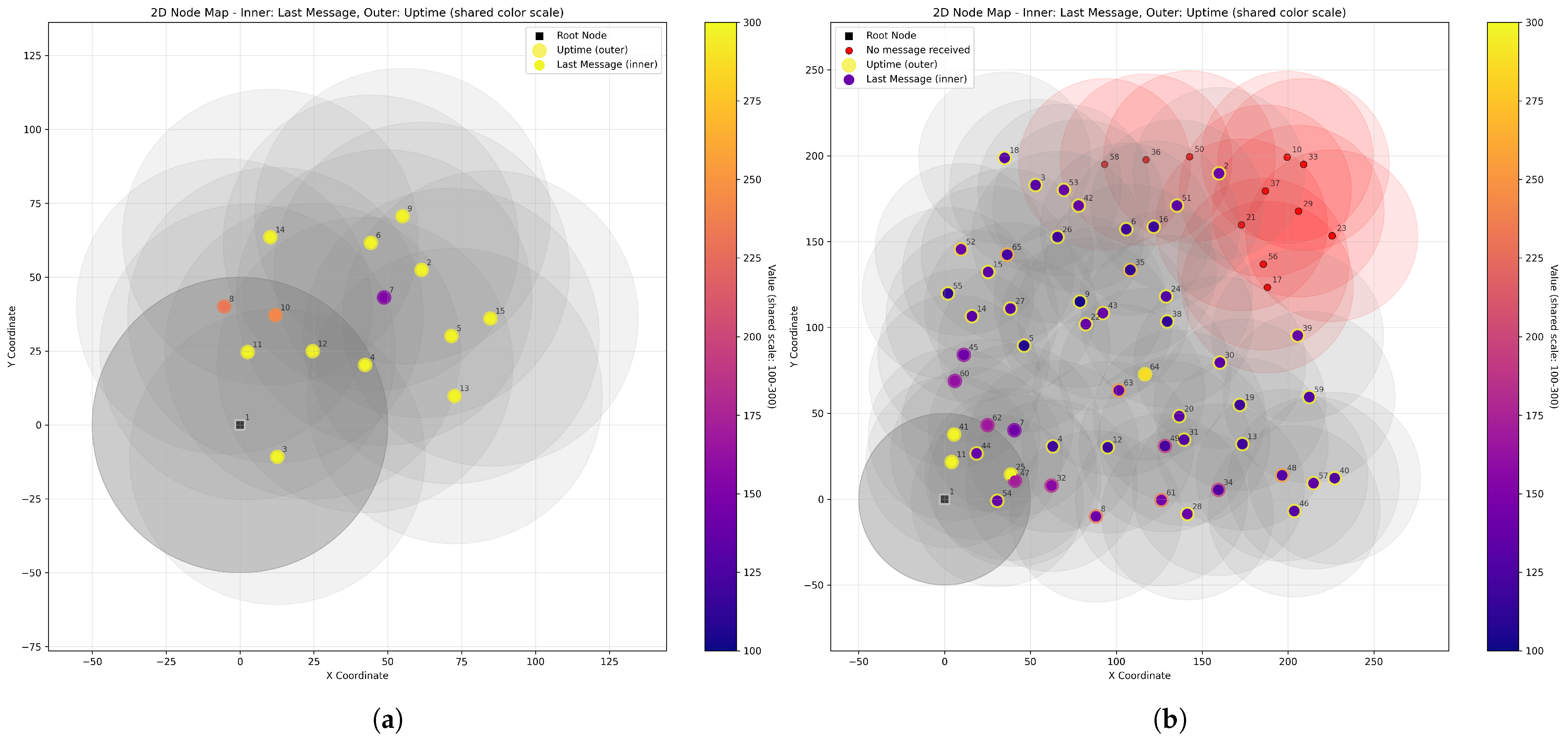
The dataset exhibits substantial diversity across multiple dimensions. Network sizes span 15 to 75 nodes with a median size of 52 nodes, enabling evaluation of scale-dependent phenomena. Two examples are shown in Figure 3. Spatial configurations vary from compact deployments (grid spacing near 20 m) to sparse layouts (spacing approaching 30 m), producing networks with two to eight neighbors per node on average. Figure 4 summarizes key dataset statistics for the training set. The other splits are similar. CPU usage varies from 0 to 80 s, averaging at around 13 s. Initial battery levels are between 25 and 100 mAh. Most nodes have 295 s of uptime (up to the end of the simulation), but around one quarter of them run out of battery earlier.
Outcome variability is quite rich. For per-node contact loss (time of last message received by root), the distribution is bimodal: approximately 13% of nodes maintain contact throughout the simulation (contact loss time = 295 s), while the remainder lose connectivity earlier due to battery depletion or network partitioning and form a skewed distribution (Figure 4). The mean contact loss time is 186.2 s with a standard deviation of 64.3 s. For network coverage, the mean final coverage is 50,333 square meters (assuming a 30 m sensing radius per operational node) with a standard deviation of 14,131 square meters, reflecting variance in both network size and spatial distribution.
Notably, the dataset captures complex failure modes: we observe instances where nodes with high battery capacity lose contact early due to relay failures upstream, and conversely, low-battery nodes that maintain connectivity throughout thanks to favorable topological positions. This complexity motivates the use of graph-structured learning: simple feature-based models or analytical methods will hardly be able to capture the interplay between spatial layout, routing dependencies, and energy heterogeneity.

3.2. Contact Loss Prediction

Arguably, the main contributing factor to the contact loss between the nodes and the root is the initial battery level. Figure 5 shows the relationship between the initial energy and the time the last message was received by the root. It is obvious that there is a linear upper bound for low initial energies, which corresponds to the uptime of that particular node. But many points are placed below the upper bound. These details are well captured by both baselines: the mean predictor and the uptime-based predictor, although neither captures the whole variance.
The GNN model is more flexible and can learn spatial relationships between nodes. Figure 6 shows the results of all three models. The mean predictor achieves slightly better performance than the uptime-based predictor (72.9 vs. 75.3 mean absolute error), and both, as expected, fail to identify nodes that do not exchange any messages with the root. The GNN is more flexible. While it still does not clearly detect nodes with no messages, the predicted contact loss times on those nodes are generally smaller than on the other nodes. The GNN gets 48.1 s of MAE on the test set, a 35% error reduction over the baselines, and achieves a decent goodness of fit ( R 2 = 0.509 ).

3.3. Network Coverage Prediction

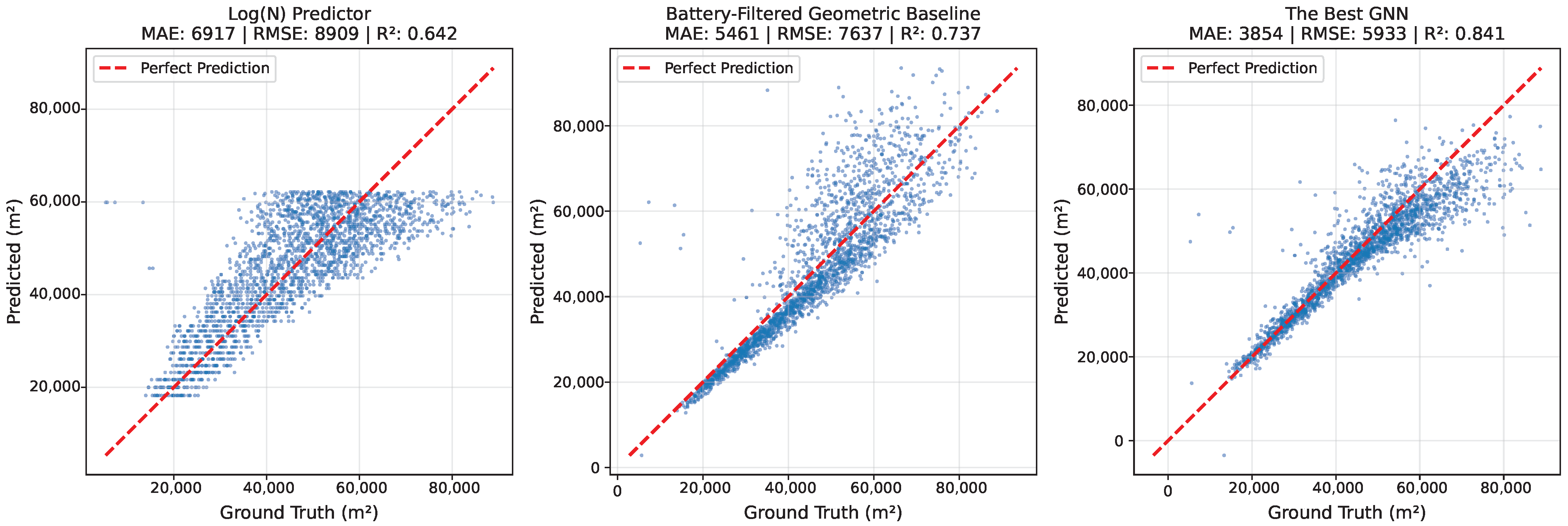
For graph-level coverage prediction, the number of nodes in the network is a decisive factor. As seen in Figure 7, the coverage area follows a sublinear trend with respect to the network size. The trend on the training set was better captured by a log ( N ) predictor, which gives 6917 square meters mean average error on the test set (6981 on the training set). As we know the locations of the nodes, we can expect the geometric baseline to perform better, especially if we filter out the nodes that have low initial battery levels. As shown in Figure 8, the battery-filtered geometric baseline is indeed better by 21% (5461 square meters MAE). The error gets significantly higher for larger networks. The GNN model achieves an MAE of 3854 square meters, again substantially outperforming baselines (almost 30% reduction in error) and achieving remarkable goodness of fit (0.841). In relative terms, this error is 8.45% of the ground truth coverage.

4. Discussion

Our results demonstrate that automated dataset generation coupled with graph neural networks can provide accurate, efficient surrogate models for IoT network behavior under resource constraints. The framework’s ability to synthesize thousands of diverse simulations highlights the value of systematic automation.
The choice of GNNs in this paper by no means should be considered optimal; we simply chose a well-known off-the-shelf model to demonstrate the power of simulated datasets. For any particular IoT problem, one might need to design and tune better-suited ML models, and the GraphSAGE-based model described in this paper can be used as a strong baseline.
After one round of dataset collection and ML model training, practitioners can avoid costly simulations and perform network analysis much faster. We performed GNN inference on NVIDIA GeForce RTX 3080 GPUs, and it took only 4.73 s to run the coverage prediction on the entire test set, giving 2.14 ms per network on average with a batch size of 32. With a batch size of 2, it gives 5.19 ms on average. That is more than an 80,000× speedup compared to a single simulation.
This speedup enables IoT design and optimization experiments that are too time-consuming with regular simulation-in-the-loop. For example, an algorithm can generate potential network configurations and use evolutionary or reinforcement-learning-based methods to optimize certain network parameters that can be computed with fast ML models for a few hundred network configurations per second. This kind of optimization is prohibitively expensive with the original simulations.

5. Conclusions

This paper presents an end-to-end pipeline for automated generation and machine-learning-based analysis of large-scale IoT network datasets, integrating parameterized topology generators, templated simulation configuration, Slurm-orchestrated distributed execution, and structured data extraction. Our case study on RPL networks demonstrates the framework’s capability to synthesize over 10,000 simulations capturing complex phenomena, including cascading relay failures and topology-dependent disconnection patterns, while graph neural networks trained on this dataset achieve substantially better predictive performance than strong baselines. The resulting surrogate models enable rapid what-if analysis, evaluating thousands of network configurations in seconds rather than days and transforming slow, serial simulation workflows into interactive design-space exploration. More broadly, this work establishes a reusable methodology for data-driven IoT network studies where the modular pipeline architecture accommodates diverse firmware, protocols, and topology generators, allowing researchers to instantiate new experiments by specifying configuration parameters rather than writing custom orchestration code. The demonstrated effectiveness of GNN-based surrogates suggests that similar approaches could accelerate analysis of other complex network phenomena where simulation provides ground truth but computational cost limits exploration. Future work will focus on applying the methodology described in this paper for real-world IoT network optimization tasks. Beyond methodological contributions, the proposed framework offers practical implications for IoT network optimization. By enabling rapid and data-driven evaluation of network behaviors, the surrogate models can be integrated into optimization loops for adaptive topology control, routing policy tuning, and proactive fault mitigation. This approach can reduce the need for exhaustive simulation campaigns, allowing network designers to identify efficient, resilient, and energy-balanced configurations in real time.

Author Contributions

Conceptualization, H.K. and T.P.R.; methodology, H.K. and T.P.R.; software, A.D., G.G. and H.K.; validation, A.D. and H.K.; investigation, H.K., A.D. and T.P.R.; data curation, H.K. and A.D.; writing—original draft preparation, A.D.; writing—review and editing, H.K. and T.P.R.; visualization, H.K.; supervision, H.K. and T.P.R.; project administration, H.K. and T.P.R.; funding acquisition, H.K. and T.P.R. All authors have read and agreed to the published version of the manuscript.

Funding

The work of H. Khachatrian and G. Grigoryan was partly supported by the RA Science Committee grant No. 22rl-052 (DISTAL). The work of T. P. Raptis was partly supported by the European Union—Next Generation EU under the Italian National Recovery and Resilience Plan (NRRP), Mission 4, Component 2, Investment 1.3, CUP B53C22003970001, partnership on “Telecommunications of the Future” (PE00000001—program “RESTART”).

Data Availability Statement

The generated dataset is publicly released at https://github.com/YerevaNN/Cooja-Automation-ML, (accessed on 20 October 2025).

Conflicts of Interest

The authors declare no conflicts of interest.

References

  1. Raptis, T.P.; Passarella, A.; Conti, M. Data Management in Industry 4.0: State of the Art and Open Challenges. IEEE Access 2019, 7, 97052–97093. [Google Scholar] [CrossRef]
  2. Koutsiamanis, R.A.; Papadopoulos, G.Z.; Fafoutis, X.; Fiore, J.M.D.; Thubert, P.; Montavont, N. From Best Effort to Deterministic Packet Delivery for Wireless Industrial IoT Networks. IEEE Trans. Ind. Inform. 2018, 14, 4468–4480. [Google Scholar] [CrossRef]
  3. Gaur, R.; Prakash, S. Performance and Parametric Analysis of IoT’s Motes with Different Network Topologies. In Proceedings of the Innovations in Electrical and Electronic Engineering, New Delhi, India, 2–3 January 2021; Mekhilef, S., Favorskaya, M., Pandey, R.K., Shaw, R.N., Eds.; Springer: Singapore, 2021; pp. 787–805. [Google Scholar]
  4. Voulgaridis, K.; Lagkas, T.; Angelopoulos, C.M.; Nikoletseas, S.E. IoT and digital circular economy: Principles, applications, and challenges. Comput. Netw. 2022, 219, 109456. [Google Scholar] [CrossRef]
  5. Osterlind, F.; Dunkels, A.; Eriksson, J.; Finne, N.; Voigt, T. Cross-level sensor network simulation with cooja. In Proceedings of the 2006 31st IEEE Conference on Local Computer Networks, Tampa, FL, USA, 14–16 November 2006; IEEE: Piscataway, NJ, USA, 2006; pp. 641–648. [Google Scholar]
  6. Oikonomou, G.; Duquennoy, S.; Elsts, A.; Eriksson, J.; Tanaka, Y.; Tsiftes, N. The Contiki-NG open source operating system for next generation IoT devices. SoftwareX 2022, 18, 101089. [Google Scholar] [CrossRef]
  7. Grigoryan, G.; Khachatrian, H.; Raptis, T.P. Toward Automating Cooja Experiment Workflows for Dataset Generation. In Proceedings of the 2024 11th International Conference on Software Defined Systems (SDS), Gran Canaria, Spain, 9–11 December 2024; pp. 19–26. [Google Scholar] [CrossRef]
  8. Essop, I.; Ribeiro, J.C.; Papaioannou, M.; Zachos, G.; Mantas, G.; Rodriguez, J. Generating Datasets for Anomaly-Based Intrusion Detection Systems in IoT and Industrial IoT Networks. Sensors 2021, 21, 1528. [Google Scholar] [CrossRef] [PubMed]
  9. Corso, G.; Stark, H.; Jegelka, S.; Jaakkola, T.; Barzilay, R. Graph neural networks. Nat. Rev. Methods Prim. 2024, 4, 17. [Google Scholar] [CrossRef]
  10. Tian, L.; Mehari, M.T.; Santi, S.; Latré, S.; De Poorter, E.; Famaey, J. Multi-objective surrogate modeling for real-time energy-efficient station grouping in IEEE 802.11ah. Pervasive Mob. Comput. 2019, 57, 33–48. [Google Scholar] [CrossRef]
  11. Ngo, D.T.; Aouedi, O.; Piamrat, K.; Hassan, T.; Raipin-Parvédy, P. Empowering Digital Twin for Future Networks with Graph Neural Networks: Overview, Enabling Technologies, Challenges, and Opportunities. Future Internet 2023, 15, 377. [Google Scholar] [CrossRef]
  12. Arzo, S.T.; Naiga, C.; Granelli, F.; Bassoli, R.; Devetsikiotis, M.; Fitzek, F.H.P. A Theoretical Discussion and Survey of Network Automation for IoT: Challenges and Opportunity. IEEE Internet Things J. 2021, 8, 12021–12045. [Google Scholar] [CrossRef]
  13. Chernyshev, M.; Baig, Z.; Bello, O.; Zeadally, S. Internet of Things (IoT): Research, Simulators, and Testbeds. IEEE Internet Things J. 2018, 5, 1637–1647. [Google Scholar] [CrossRef]
  14. Almutairi, R.; Bergami, G.; Morgan, G. Advancements and Challenges in IoT Simulators: A Comprehensive Review. Sensors 2024, 24, 1511. [Google Scholar] [CrossRef] [PubMed]
  15. Jha, D.N.; Alwasel, K.; Alshoshan, A.; Huang, X.; Naha, R.K.; Battula, S.K.; Garg, S.; Puthal, D.; James, P.; Zomaya, A.; et al. IoTSim-Edge: A simulation framework for modeling the behavior of Internet of Things and edge computing environments. Softw. Pract. Exp. 2020, 50, 844–867. [Google Scholar] [CrossRef]
  16. Mahmud, R.; Pallewatta, S.; Goudarzi, M.; Buyya, R. iFogSim2: An extended iFogSim simulator for mobility, clustering, and microservice management in edge and fog computing environments. J. Syst. Softw. 2022, 190, 111351. [Google Scholar] [CrossRef]
  17. Levis, P.; Lee, N.; Welsh, M.; Culler, D. TOSSIM: Accurate and scalable simulation of entire TinyOS applications. In Proceedings of the SenSys ’03: Proceedings of the 1st International Conference on Embedded Networked Sensor Systems, Los Angeles, CA, USA, 5–7 November 2003; pp. 126–137. [Google Scholar] [CrossRef]
  18. Dunkels, A.; Osterlind, F.; Tsiftes, N.; He, Z. Software-based on-line energy estimation for sensor nodes. In Proceedings of the 4th Workshop on Embedded Networked Sensors, Cork, Ireland, 25–26 June 2007; pp. 28–32. [Google Scholar]
  19. Moteiv Corporation. Tmote Sky Wireless Sensor Node Datasheet. 2006. Available online: http://www.crew-project.eu/sites/default/files/tmote-sky-datasheet.pdf (accessed on 6 October 2025).
  20. Hamilton, W.; Ying, Z.; Leskovec, J. Inductive representation learning on large graphs. In Proceedings of the 31st International Conference on Neural Information Processing Systems, Long Beach, CA, USA, 4–9 December 2017; Volume 30. [Google Scholar]
  21. Rusch, T.K.; Bronstein, M.M.; Mishra, S. A survey on oversmoothing in graph neural networks. arXiv 2023, arXiv:2303.10993. [Google Scholar] [CrossRef]
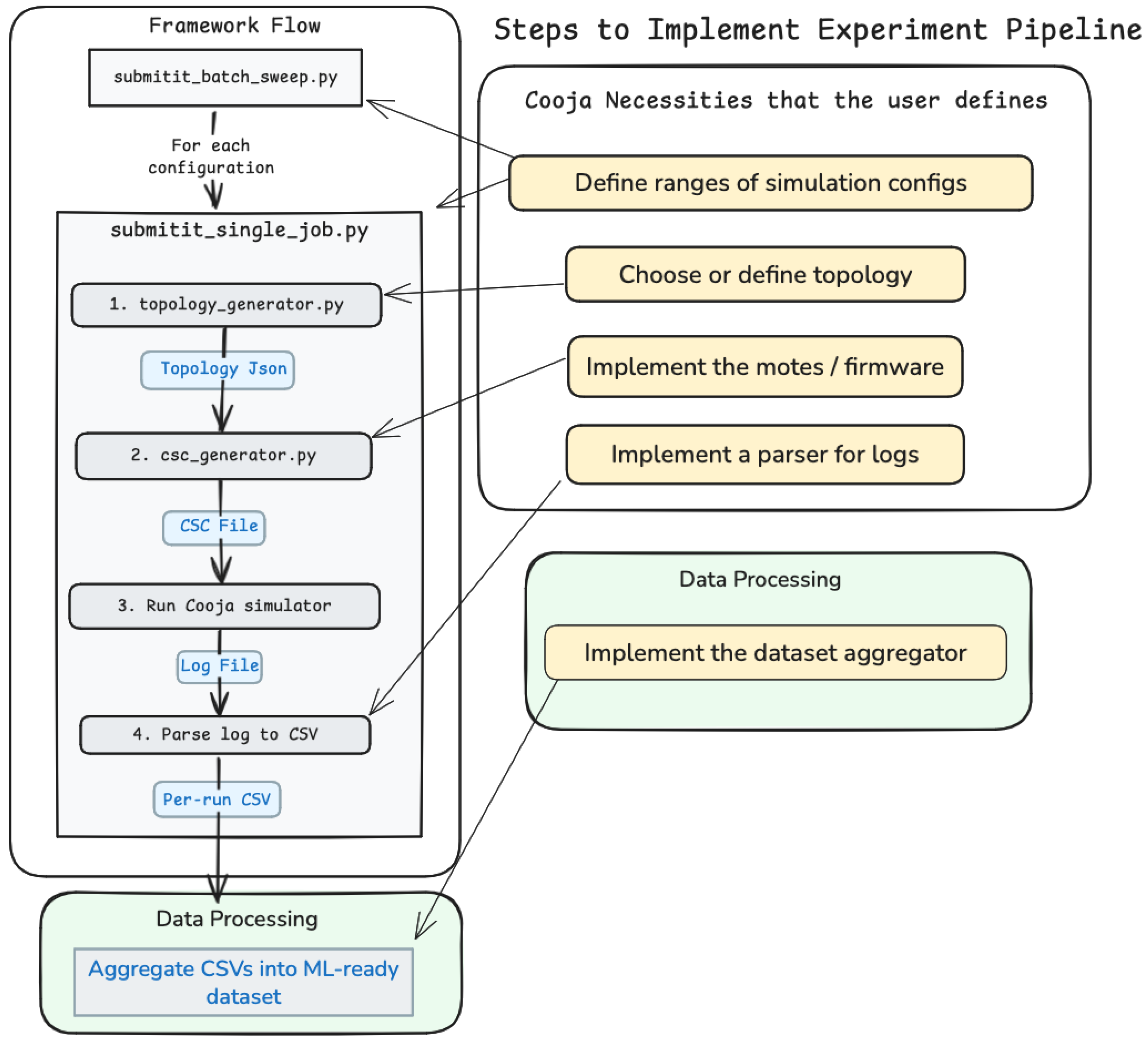
Figure 1. Automation pipeline: topology JSON → CSC → Cooja log → parsed CSV → optional DB. User inputs (yellow) and optional components (dashed) are indicated.
Futureinternet 17 00518 g001
Figure 2. Distribution of simulation runtimes. Simulations take longer for larger networks.
Futureinternet 17 00518 g002
Figure 3. Two network simulations with N = 15 (a) and N = 75 (b) nodes. Each dot has two colors; the inner circle denotes the time the last message was received by the root node (aka contact loss), while the outer circle denotes the uptime. For some nodes, these two values are equal, while other nodes stay alive long after the root loses contact with them.
Futureinternet 17 00518 g003
Figure 4. Basic statistics of the simulations from the training split of the dataset we have generated.
Futureinternet 17 00518 g004
Figure 5. Contact loss vs. initial battery energy across all simulations in the training set. Red line shows the average contact loss time for each initial battery level, which serves as the mean predictor baseline. Green dashed line shows the uptime-based baseline (uptime divided by 1.5).
Futureinternet 17 00518 g005
Figure 6. Contact loss prediction models. GNN significantly outperforms the two baselines.
Futureinternet 17 00518 g006
Figure 7. Linear and sublinear coverage baselines. Log(N) fits the training set better compared to sqrt and linear.
Futureinternet 17 00518 g007
Figure 8. Coverage prediction models. The geometric baseline already achieves a strong goodness of fit, while the GNN reduces mean absolute error (MAE) by approximately 30%.
Futureinternet 17 00518 g008
Table 1. Customization points in the automation pipeline.
ComponentDescription
Firmware (required)Source code for sink and sensing motes (src/*.c).
Topology definition (required)Topology family and parameter ranges (e.g., grid, tree, random mesh).
Sweep configuration (required)Duration, seeds, radio and battery settings.
Parser (required)Adjusts to firmware-specific log message formats.
Dataset builder (optional)Aggregates parsed results into ML-ready datasets.
Database loader (optional)Inserts processed data into PostgreSQL tables.
Table 2. A typical example of a CSV produced the log parser that describes a single simulation with 18 nodes.
MotexyCPULPMListenTransmitOffTotalInitial
Battery
ConsumedRemainingStatusUptimeLast msg
recv
by Root
SentForwarded
10.00.01726828500285 2 32 0 2 32 alive285 00
276.0115.41727829401295844935alive295152169
318.9130.2329229401295734924alive295297430
414.1−3.2628929401295864937alive295297490
542.329.2928629401295994950alive2952974936
6−5.258.8429129401295884939alive295297450
739.7107.051491540115525250dead1551521862
821.173.952302340123538390dead235232340
982.3108.7182772931129551492alive2951521718
1085.323.842412440124540400dead245237350
1116.281.372882940129553494alive2952974529
1231.022.82626929401295664917alive29529752396
1350.0−5.772882940129555496alive2952975037
1447.764.9928629401295684919alive2952974982
1587.3135.41528029401295814932alive2951521310
1618.144.01328229401295704921alive29529748121
1773.510.3529029401295834934alive295297500
1860.211.7529029401295964947alive295297480
Table 3. Grid Search of the Hyperparameters of the GNN.
HyperparameterValues of the GridSelected Value for
Contact Loss Prediction
Selected Value for
Coverage Prediction
Learning rate { 10 4 , 5 · 10 4 , 10 3 } 10 4 5 · 10 4
Number of layers L { 2 , 4 , 8 } 44
Hidden dimension H { 128 , 512 } 128512
Disclaimer/Publisher’s Note: The statements, opinions and data contained in all publications are solely those of the individual author(s) and contributor(s) and not of MDPI and/or the editor(s). MDPI and/or the editor(s) disclaim responsibility for any injury to people or property resulting from any ideas, methods, instructions or products referred to in the content.