Article

Early Ransomware Detection with Deep Learning Models

Department of Software Engineering, Shamoon College of Engineering, Beer Sheva 84100, Israel
*
Author to whom correspondence should be addressed.
These authors contributed equally to this work.
Future Internet 2024, 16(8), 291; https://doi.org/10.3390/fi16080291
Submission received: 20 July 2024 / Revised: 5 August 2024 / Accepted: 9 August 2024 / Published: 11 August 2024
(This article belongs to the Special Issue Generative Artificial Intelligence (AI) for Cybersecurity)

Abstract

:
Ransomware is a growing-in-popularity type of malware that restricts access to the victim’s system or data until a ransom is paid. Traditional detection methods rely on analyzing the malware’s content, but these methods are ineffective against unknown or zero-day malware. Therefore, zero-day malware detection typically involves observing the malware’s behavior, specifically the sequence of application programming interface (API) calls it makes, such as reading and writing files or enumerating directories. While previous studies have used machine learning (ML) techniques to classify API call sequences, they have only considered the API call name. This paper systematically compares various subsets of API call features, different ML techniques, and context-window sizes to identify the optimal ransomware classifier. Our findings indicate that a context-window size of 7 is ideal, and the most effective ML techniques are CNN and LSTM. Additionally, augmenting the API call name with the operation result significantly enhances the classifier’s precision. Performance analysis suggests that this classifier can be effectively applied in real-time scenarios.

Graphical Abstract

1. Introduction

Ransomware (RW) is malware that prevents access to a computer system or data until a ransom is paid. It is primarily spread via phishing emails and system flaws, and it has a serious negative impact on individuals and companies that use computer systems daily [1,2,3].
In general, ransomware can be divided into two main types. The first type is called locker ransomware. It aims to deny access to a computer system but does not encrypt files. This type of RW blocks users from the system interface and locks them out of their work environments and applications [4]. The second type is called crypto ransomware. It encrypts valuable data in the system, such as documents and media files, and it renders them inaccessible without a decryption key. This is the dominant form of RW because of its devastating effect on data integrity [4].
The effects of ransomware attacks go beyond the money lost as soon as the ransom is paid. Operational interruptions can cause major productivity losses for organizations, particularly in vital industries like healthcare [1,2,5]. In addition, victims may experience intense psychological effects, including feelings of anxiety and violation [2]. Ransomware is a profitable business for hackers because the costs of downtime, data loss, and system recovery frequently outweigh the ransom payment itself [6]. The rate of ransomware attacks has increased significantly; in 2017, an attack occurred somewhere in the world every 40 s, and by 2019, this frequency had escalated to every 19 s [7]. Financial losses due to ransomware attacks were $8 billion in 2018 and over $20 billion by 2021 [8]. Ransom demands range from a few hundred dollars for personal computers to up to a million dollars for enterprises [9], with victims facing potential losses of hundreds of millions of dollars if they do not pay. The first reported death following a ransomware attack occurred at a German hospital in October 2020 [10].
Given the sophisticated and evolving nature of ransomware, understanding its mechanics and impacts is crucial. This includes recognizing how it can infiltrate systems, the variety of its types, and the extensive consequences of attacks. Therefore, effective detection and mitigation strategies are essential when malicious activity starts. This paper contributes to these efforts by employing deep learning techniques to detect and analyze ransomware based on system behavior and response patterns within the first few seconds of its activity.
Deep learning (DL) is an excellent tool for spotting subtle and complicated patterns in data, which is important for detecting zero-day ransomware assaults [11,12]. Once trained, deep learning models can handle enormous amounts of data at rates faster than human analysts, making them perfect for real-time threat identification. These models can also identify new and changing threats over time. But big, well-labeled datasets are necessary for efficient deep learning applications, and their preparation can be costly and time-consuming [13]. Additionally, there is a chance that models will overfit, which would hinder their ability to be generalized to fresh, untested data. Finally, training deep learning models demands substantial computational resources, which can be an obstacle for some organizations [14].
Ransomware often performs operations repeatedly, for example, file scanning and the encryption of multiple directories. This conduct implies that RW contains consistent and detectable behavioral patterns. These patterns subtly evolve with each RW variant, presenting an ideal use case for deep learning models, especially those designed for sequence analysis. Moreover, the relative ease of modifying existing ransomware toolkits allows attackers to rapidly develop new variants [15]. Deep learning’s capability to learn from incremental data adjustments makes it highly effective at identifying slight deviations from known behaviors, offering a robust defense against an ever-evolving ransomware landscape.
In this paper, we present a new dataset and a method for early ransomware detection. Our contribution is three-fold. First, we have created a comprehensive dataset featuring a wide array of initial API call sequences from commonly used benign and verified crypto-ransomware processes. This dataset is unique not only in its verification process, ensuring that all included ransomware samples are 100% validated as crypto-ransomware, but also in the depth of data recorded for each API call. It includes detailed information such as the result of each call, its duration, and the parameters involved. The public release of this dataset will make it a useful tool for researchers, enabling them to make even more progress in ransomware detection and stronger protection system development. Second, we have conducted a detailed comparative analysis of various neural network configurations and dataset features. This analysis aims to determine the most effective neural network model and feature set for ransomware detection. Third, we detect ransomware processes using initial API call sequences of a process and obtain an efficient method of early ransomware detection.
We examine the following research questions (RQs):
RQ1:
What API call features are essential for early ransomware detection?
RQ2:
Do neural models outperform traditional machine learning (ML) models for this task?
RQ3:
What representation of textual API call features yields better results?
RQ4:
What number of consecutive API calls from every process is sufficient for state-of-the-art results?
RQ5:
Are test times for neural models competitive and suitable for online ransomware detection?
Due to the scarcity of available datasets and code, we decided to share both in order to facilitate further research in the field. Both data and code will be publicly available when this paper is published.

2. Background

Traditionally, ransomware detection methods have relied on several key strategies. Signature-based detectionis the most common method used in traditional antivirus software. It matches known malware signatures—unique strings of data or characteristics of known malware—against files. While effective against known threats, this method struggles to detect new, unknown ransomware variants [16,17]. Heuristic analysis uses algorithms to examine software or file behavior for suspicious characteristics. This method can potentially identify new ransomware based on behaviors similar to known malware, but its effectiveness depends on the sophistication of the heuristic rules [18]. Behavioral analysis monitors how programs behave and highlights odd behaviors—like quick file encryption—that could indicate ransomware. Although these tools need a baseline of typical behavior and can produce false positives, they may identify zero-day ransomware attacks (new and undiscovered threats) [18]. Sandboxing runs files or programs in a virtual environment (sandbox) to observe their behavior without risking the actual system. If malicious activities like unauthorized encryption are detected, the ransomware can be identified before it harms the real environment. However, some advanced ransomware can detect and evade sandboxes [19]. Honeyfiles (decoy folders) places decoy files or folders within a system. Monitoring these decoys for unauthorized encryption or modifications can signal a ransomware attack. While useful as an early warning system, it does not prevent ransomware from infecting genuine files [20].
Although each of these approaches has advantages, they also come with special difficulties when it comes to ransomware detection. One major obstacle is finding a balance between the necessity for quick, precise detection and the reduction in false positives and negatives. For this purpose, machine learning technologies, especially deep learning (DL), are now used because they provide strong defenses against ransomware and other sophisticated cyber threats. DL is used in malware classification [21], phishing detection [22], anomaly identification [23], and malware detection. By examining the order of operations in a system, which may include odd file-encryption activities, DL models have demonstrated high efficacy in detecting ransomware activities [24,25]. DL can spot subtle and complicated patterns in data, which is important for detecting zero-day ransomware assaults; it can also handle enormous amounts of data, making it perfect for real-time threat identification. However, big and well-labeled datasets are necessary for efficient DL models, and their preparation can be costly and time-consuming [13]. Additionally, there is a chance that models will overfit and not generalize well on fresh and untested data. Training DL models demands substantial computational resources, which can be an obstacle for some organizations [14].
Next, we survey some of the most prominent works on ML-based ransomware detection. The study [26] significantly extends the realm of cybersecurity by utilizing an advanced dataset consisting of both ransomware and benign software samples collected from 2014 to early 2021. These samples underwent dynamic analysis to document API call sequences, capturing detailed behavioral footprints. The LightGBM model was used to classify the samples. The model demonstrated exceptional efficacy, achieving an accuracy of 0.987 in classifying software types.
The work [27] presents a sophisticated approach to malware detection by distinguishing API call sequences using long short-term memory (LSTM) networks, which were not limited to ransomware. The dataset in this paper was sourced from Alibaba Cloud’s cybersecurity efforts, and it contains a comprehensive collection of malware samples, including ransomware. The dataset spans various malware types, and it includes dynamic API call sequences from malware, capturing only the names of the API calls while omitting additional details such as call results or timestamps. API call sequences are mapped from strings into vectors using an API2Vec vectorization method based on Word2Vec [28]. The LSTM-based model of [27] achieved an F1-score of 0.9402 on the test set, and it was shown to be notably superior to traditional machine learning models.
The paper [29] introduces an innovative approach to malware detection using deep graph convolutional neural networks (DGCNNs) [30]. It focuses on the capabilities of DGCNNs to process and analyze API call sequences. The dataset used in this work comprises 42,797 malware API call sequences and 1079 goodware API call sequences; only the API call names were recorded. DGCNNs demonstrated comparable accuracy and predictive capabilities to LSTMs, achieving slightly higher F1 scores on the balanced dataset but performing less well on the imbalanced dataset.
The work [31] concentrates on the behavioral analysis of both malicious and benign software through API call monitoring. Instead of analyzing the sequence of API calls, this study employs advanced machine learning techniques to assess the overall frequency and type counts of these API calls. The authors developed two distinct datasets that include a wide variety of ransomware families. The datasets contain only API call names. Several ML algorithms were tested, including k-nearest neighbors (kNNs) [32], random forest (RF) [33], support vector machine (SVM) [34], and logistic regression (LR) algorithms [35]. Both LR and SVM exhibited exemplary performance, achieving perfect precision scores of 1.000 and the highest recall rates of 0.987, which correspond to an F1-score of 0.994.
In the paper [29], the authors propose a novel behavioral malware detection method based on deep graph convolutional neural networks (DGCNNs) to learn directly from API call sequences and their associated behavioral graphs. They use longer call sequences (100 API calls) to achieve high classification accuracy and F1 scores on a custom dataset of over 40,000 API call sequences.
The goal of this paper is to improve detection skills by combining deep learning with the fundamentals of behavioral analysis. This will lessen the possibility of false positives and improve the identification of zero-day threats.

3. PARSEC Dataset

3.1. Motivation

One of the primary reasons for opting to collect our data, rather than using pre-built datasets, was the lack of available datasets that include detailed outcomes of API calls. Most publicly available datasets (described in Section 2) typically provide only the names of the API calls made during the execution of malware and benign applications. We made an effort to find a dataset that would fit our research. The reviewed datasets were MalBehavD-V1 [36], the Malware API Call Dataset [37], the Alibaba Cloud Malware Detection Based on Behaviors Dataset [38], and the datasets introduced in papers [29,39]. None of these datasets were suitable for our purposes because they only provided the names of API calls. In our study, we wanted to explore the effect of additional information, such as the result of the API call, its duration, and the parameters it received, to see whether these additional details could improve performance metrics in ransomware detection.
However, for a more nuanced analysis and potentially more effective detection models, it is crucial to consider not only the API calls themselves but also their results, the duration of each call, and its parameters. This is why we present a new dataset named PARSEC, which stands for API calls for ransomware detection.

3.2. Data Collection

We chose to use Windows 7 for malware analysis because, despite being an older operating system, it remains a target for malware attacks due to its widespread use in slower-to-upgrade environments [40]. Therefore, malware analysis on Windows 7 provides insights into threats still exploiting older systems. Additionally, many malware variants designed to target Windows platforms maintain compatibility with Windows 7 due to its architectural similarities with newer versions. Note that our method and results are also applicable to the Windows 10 OS and its server counterparts. It is important to note that, for our purposes, Windows 7 and Windows 10 are API-compatible. This means a sample identified as ransomware on Windows 7 would also be classified as ransomware on Windows 10.
We used Process Monitor [41] (PM) on a Windows 7 Service Pack 1 (SP1) environment within VirtualBox v6.1 [42] to record API calls from both benign and malicious processes. Process Monitor (v3.70) is a sophisticated tool developed by Sysinternals (now part of Microsoft) that can capture detailed API call information [43].
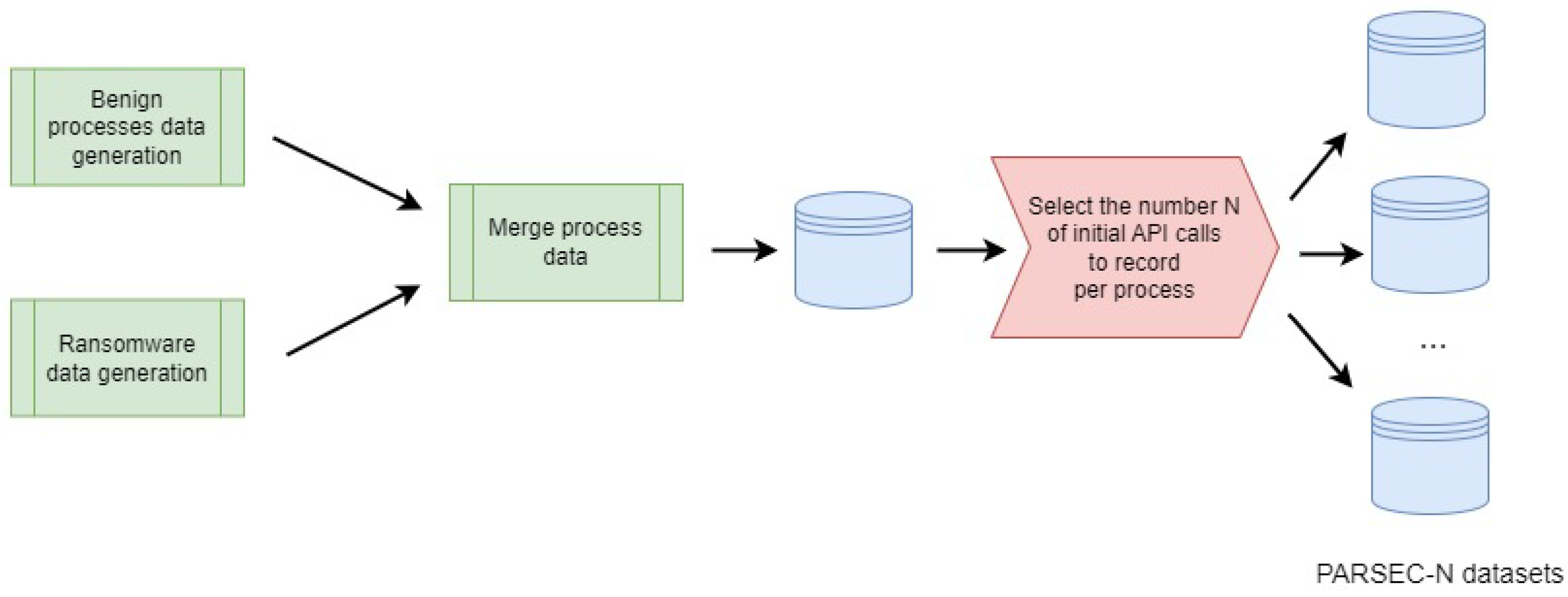
We collected the data for malicious and benign processes separately. For each API call of a process, we recorded the call’s name, result, parameters, and execution time. Then, we filtered the API calls and their parameters from every process to construct our datasets; this procedure is shown in detail below. Figure 1 shows the pipeline of our data collection.
Note that our set of ransomware and benign processes is extensive, but it does not contain all possible processes. However, choosing a few representatives from each application group is an acceptable practice in benchmarking, and we consider the selected set of benign applications to be adequately representative. While ransomware can theoretically differ significantly, in practice, it generally follows the same patterns as other malware. There are several notable examples, such as Locky, WannaCry, and Ryuk, from which all others are derived [44,45].

3.3. Benign Processes

We selected a diverse suite of 62 benign processes to capture a broad spectrum of normal computer activities. This selection strategy was aimed at ensuring that our dataset accurately reflects the varied operational behaviors a system might exhibit under different scenarios, including active user interactions and passive background tasks. These processes belong to five main types described below.
  • Common applications, such as 7zip (v22.01), axCrypt (v2.1.16.36), and CobianSoft (v2.3.10), are renowned for their encryption and backup capabilities. These choices are important for studying legitimate encryption activities, as opposed to the malicious encryptions conducted through ransomware.
  • Utility and multimedia tools, such as curl (for downloading tasks) and ffmpeg (v.3, for multimedia processing), are crucial for representing standard, non-malicious API call patterns that occur during routine operations.
  • Office applications like Excel (office professional plus 2010) and Word (office professional plus 2010) reflect common document-handling activities–normal document access and modification patterns.
  • Benchmarking applications such as Passmark (v9) and PCMark7 (v1.4.0) simulate a wide array of system activities, from user engagement to system performance tests. These applications provide a backdrop of benign system-stress scenarios.
  • Idle-state processes that typically run during the computer’s idle state represent the system’s behavior when it is not actively engaged in user-directed tasks. This category is essential for offering insights into the system’s baseline activities.
The full list of benign processes appears in Appendix A.1 of Appendix A.

3.4. Ransomware Processes

We started from a dataset comprising 38,152 ransomware samples, obtained from VirusShare.com [46]. To verify this site’s virus classification, we employed an automated pipeline to verify the authenticity of these samples as ransomware. The objective was to identify at least 62 ransomware programs within this dataset to match the number of benign processes described in Appendix A.1. The identification pipeline is a multi-stage process designed to differentiate actual ransomware from potential threats. It includes two VirtualBox virtual machines (VMs) and a host machine, each playing a critical role in screening, analyzing behavior, and confirming ransomware candidates. The full pipeline of ransomware API calls collection flow is shown in Figure 2.
The first virtual machine (denoted as VM1) starts the process by querying the VirusTotal API for each entry in the “VirusShare_CryptoRansom_20160715” collection, which consists of 38,152 potential samples. Its objective is to filter and prioritize samples based on the frequency of detections via various antivirus engines. Prioritized samples are forwarded to the second virtual machine (denoted as VM2) for a detailed behavioral analysis.
VM2 receives prioritized samples (one by one) from VM1 and executes each in a secure, controlled setting. It focuses on detecting encryption attempts targeting a “honey spot,” which refers to a deliberately crafted and strategically placed element within a system or network designed to attract ransomware or malicious activities [47]. All API calls made during execution are recorded. If a sample is confirmed as ransomware (i.e., it encrypts the “honey spot”), VM2 compresses the API call data into an Excel file, packages it with WinRAR, and sends it back to VM1.
The host machine maintains a consistent testing environment by resetting VM2 after each analysis. It gathers the compressed Excel files containing API call data from confirmed ransomware samples and compiles them into a single list of these verified programs. This process resulted in a dataset of 62 validated ransomware programs from the initial 38,152 candidates after it ran for two weeks.

3.5. Dataset Features

From the collected API calls of the PARSEC dataset, we generated several datasets that differ in the number of API calls taken from each process. We selected N initial API calls of processes to enable our models to detect malicious processes upon their startup; here, N is a parameter. The aim of our approach is the early detection of ransomware processes. If a process executes fewer API calls than required for the dataset, we performed data augmentation using oversampling. Specifically, we replicated sequences of API calls at random; this method guarantees datasets’ consistency.
We selected a number of API calls between 500 and 5000 to evaluate the potential for early ransomware detection based on limited API calls. It also helped us understand the implications of dataset size on the efficiency of our models. Note that the dataset size primarily affects the duration of training. Larger volumes of data extend the training time but may result in models that are better at generalizing across different ransomware behaviors. Conversely, smaller datasets reduce the training time but might limit the model’s comprehensiveness in learning varied ransomware patterns. This balance is crucial for developing practical, deployable models that can be updated and retrained as new ransomware threats emerge. The naming convention for dataset variations is PARSEC-N, where N is the number of initial API calls included for each process. Therefore, we have PARSEC-N datasets for N = 500 , 1000 , 2000 , 3000 , 4000 , 5000 .
The API features we recorded include process operation, process result, process duration, and process detail features (a full list of these features appears in Appendix A.2). We denote these feature lists as Ops, Res, Dur, and Det, meaning operations, results, duration, and detail features. In the basic setup, we started with operation features and only extended the list by adding the result features, and then we added the API execution times and detail features. By starting with basic features and incrementally adding complexity, we isolated the impact of each feature type on the models’ performance. We denote as FLIST the list of features used in the dataset; it accepts the values Ops (process operation features), OpsRes (process operation and result features), OpsResDur (process operation, result, and duration features), and OpsResDurDet (process operation, result, duration, and detail features).

3.6. Data Representation

API call names, results, and execution times were directly extracted from the raw data without modification. Process details’ features are long strings representing the parameters passed to each API call in a semi-structured format. Each parameter is delimited with a semicolon (“;”), with key–value pairs within these parameters separated by a colon (“:”). The value of each key varied, ranging from numbers to single words or even phrases. To accurately interpret and utilize this information, we implemented a detailed extraction process:
  • First, we separated and extracted each parameter and its corresponding key–value pairs.
  • Then, we filtered out identifiable information—parameters that could serve as identifiers or indicate specific timestamps were meticulously removed to maintain the integrity of the dataset and ensure privacy compliance. The full list of these parameters can be found in Appendix A.2 of Appendix A.
  • We filled in the missing data with sequences of zeros.
  • Due to the heterogeneous nature of API calls, they might be associated with a set of parameters of different sizes. Therefore, API calls with missing parameters were systematically padded with zeros.
After feature extraction, we normalized the numerical features (such as execution times) using min-max normalization.
We used 1-hot encoding, FastText [48], and Bidirectional Encoder Representations from Transformers (BERT) sentence embeddings [49] (BERT SE) to represent text features. For FastText representation, we split all string attributes into separate words, according to camel case patterns, punctuation, tabs, and spaces, as in “END OF FILE.” The text was kept in its original case. Then, we extracted the k-dimensional word vector of every word and computed its average vector. We used fastText vectors pre-trained on English webcrawl and Wikipedia of length k = 300 . For BERT SE representation, the words were split based on camel cases and spaces, and then all strings representing words were transformed into lowercase. Then, we applied a pre-trained model bert-base-uncased and extracted vectors of length 768 for every text.
Next, we divided the data into fixed-size windows of size W. We explored four window sizes, with W = 1 , 3 , 5 , 7 . To maintain consistency across the dataset and ensure integrity in the windowed structure, we applied zero-padding where necessary. This is particularly important for the final segments of data sequences, which may not be fully populated due to variability in API call frequencies. The full data representation pipeline is depicted in Figure 3.

3.7. Data Analysis

We performed a visual and numeric analysis of our datasets to assess the quality and behavior of benign and ransomware processes. We focused on two datasets—PARSEC-500 and PARSEC-5000—that represent the smallest and biggest numbers of initial API calls taken from each process.
Table 1 contains the number of API calls performed by benign and ransomware processes for the PARSEC-500 and PARSEC-5000 datasets. We omitted the calls that were never performed through ransomware processes from this table (the full list of these calls is provided in Appendix A.3 of Appendix A). We can see, surprisingly, that the same calls appear when the first 500 API calls are taken (PARSEC-500) or the first 5000 (PARSEC-5000). It is also evident, in total, ransomware processes perform much more CloseFile, CreateFile, and IRP_MJ_CLOSE than benign processes do. They, however, perform fewer ReadFile operations than benign processes, regardless of the number of system calls recorded.
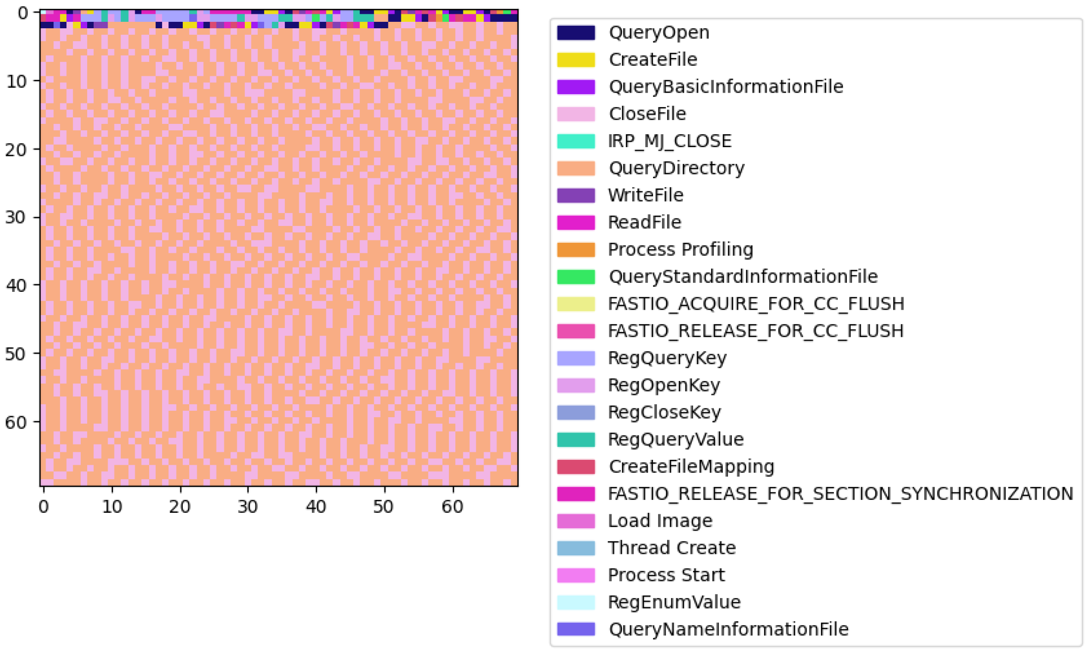
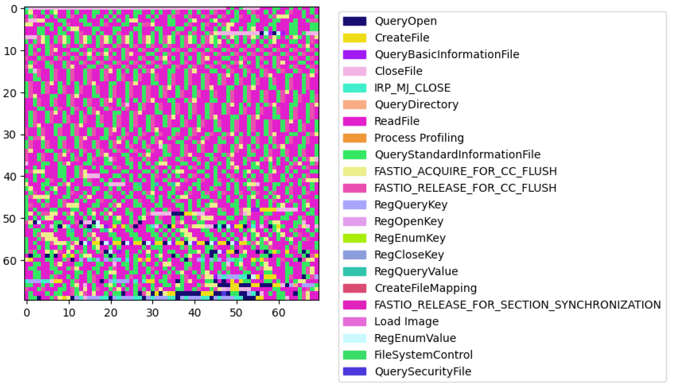
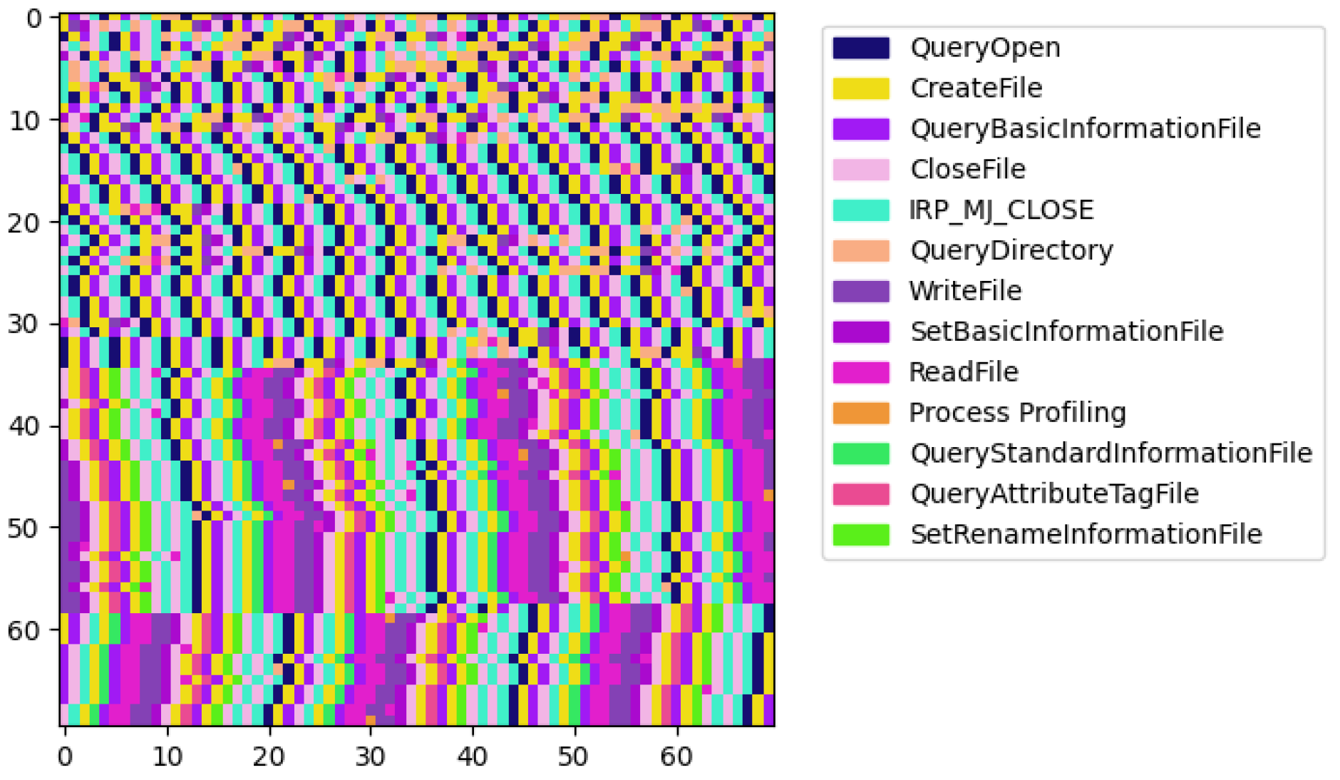
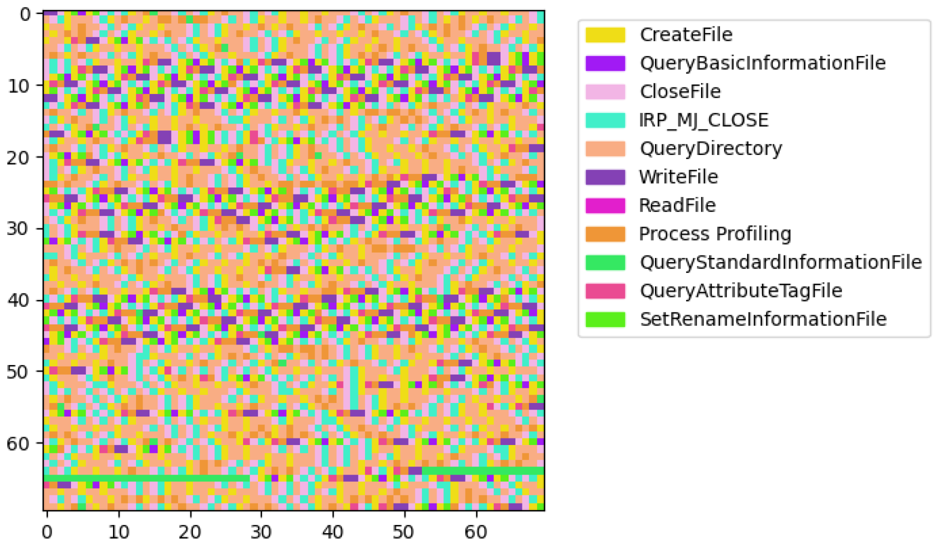
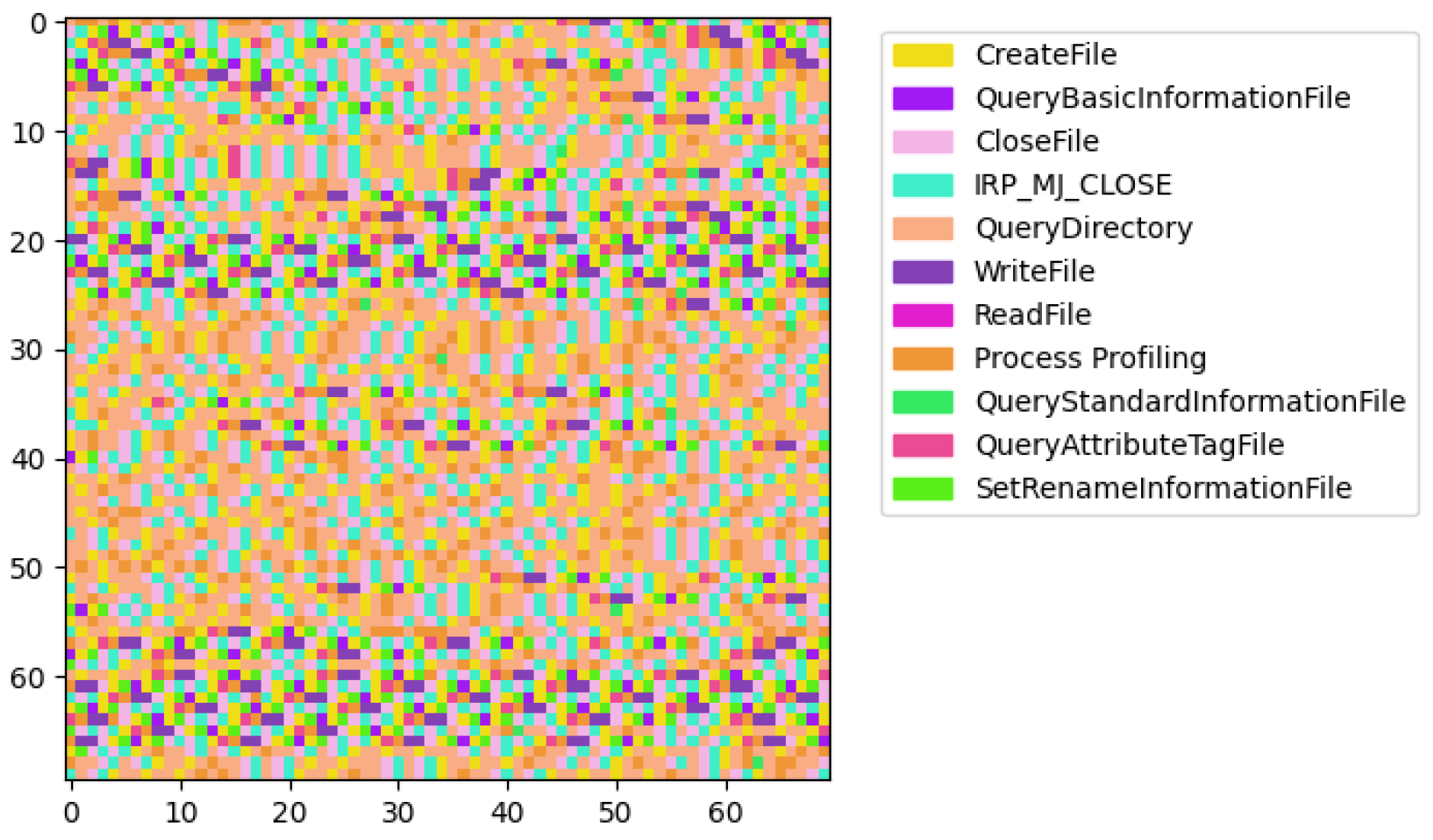
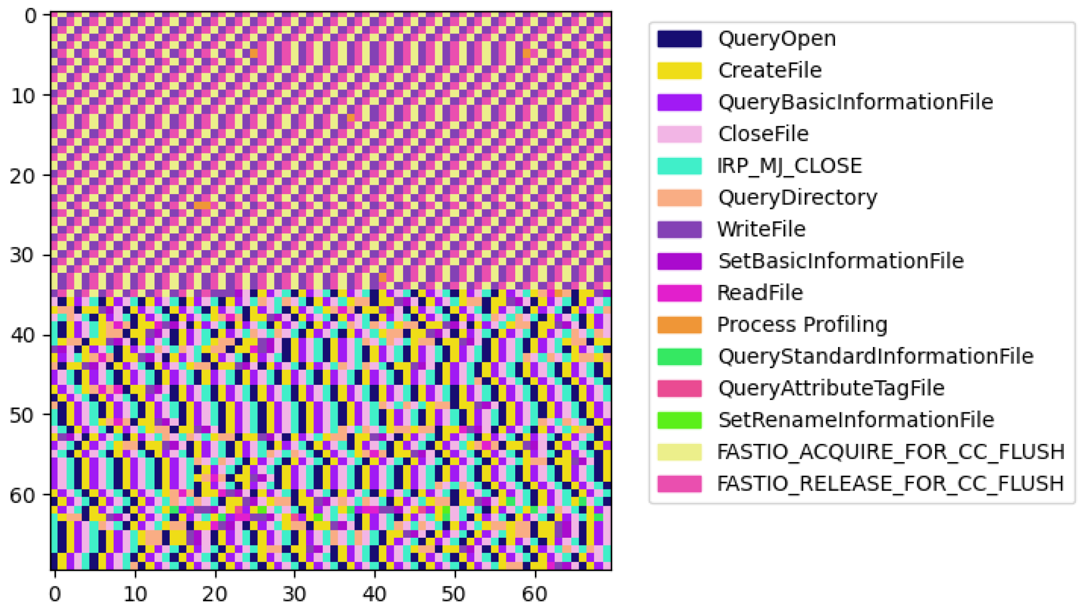
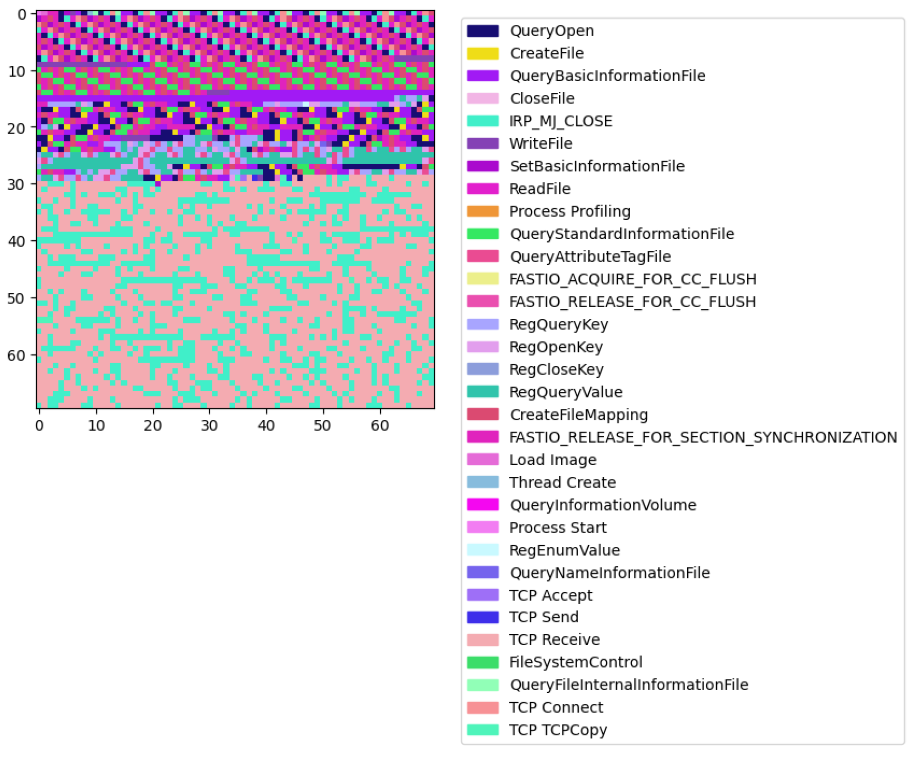
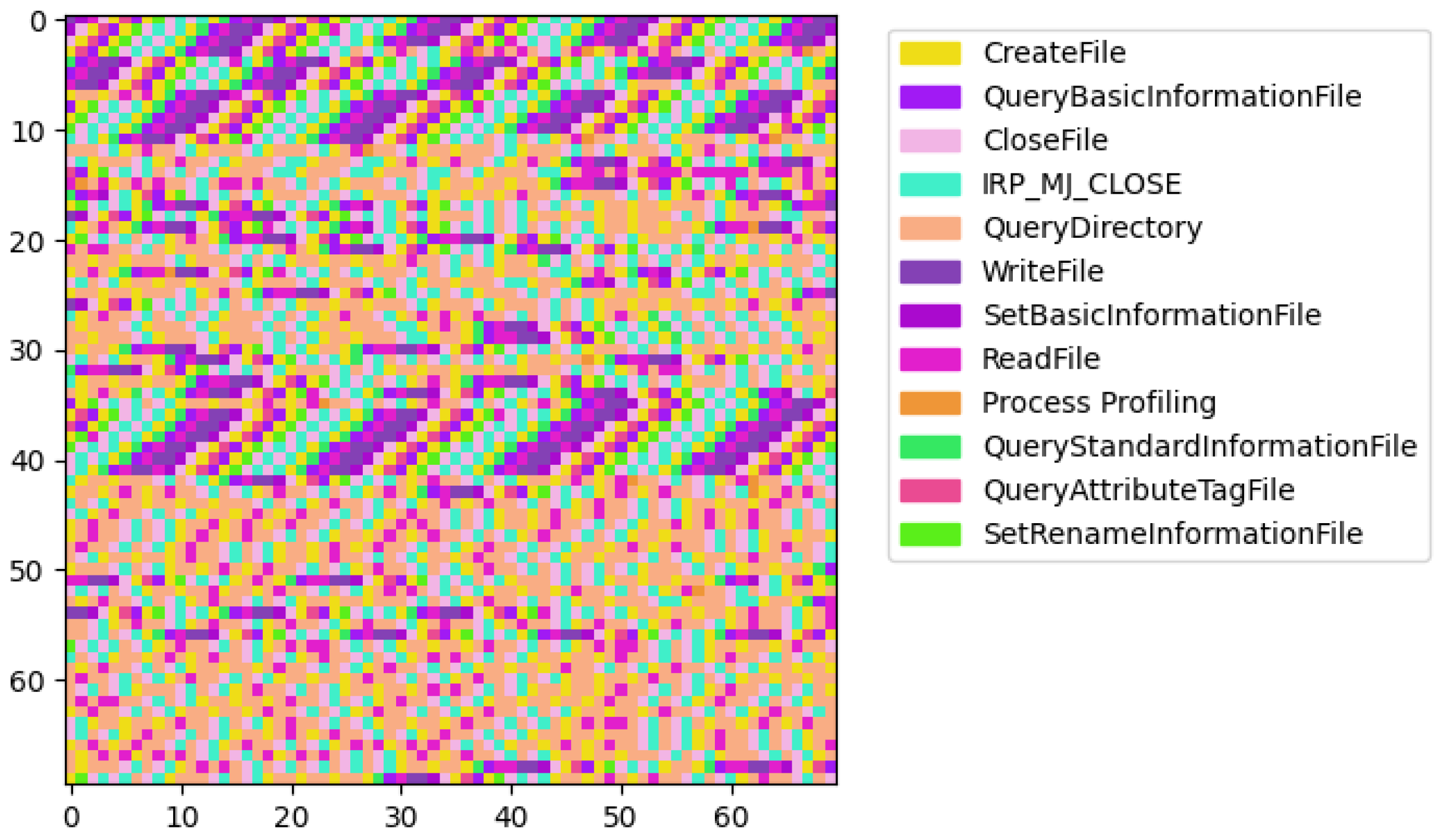
Next, we performed a visual analysis to reveal distinguishing malware characteristics. For each process, we generated a square image where each pixel represents an API call, color-coded according to the operation performed. The images were plotted with legends, associating each color with its respective API call operation. The visual analysis revealed a stark contrast between benign and ransomware processes. Benign processes exhibited a diverse array of patterns, reflecting the wide-ranging legitimate functionalities and interactions within the system. Each benign process presents a unique color distribution, illustrating the variability and complexity of non-malicious software operations. An example is shown in Figure 4. Visualization of other benign processes appears in Appendix A.4 of Appendix A.
In contrast, ransomware processes displayed a more homogenous appearance, with similar color distributions among them. This uniformity suggests a narrower set of operations being executed, which could be indicative of the focused, malicious intent of these processes. Remarkably, the ransomware processes can be grouped into a few distinct types based on the visualization of their operational sequences, suggesting the existence of common strategies employed across different malware samples.
The first type of malware (Figure 5) prominently features operations like QueryBasicInformationFile, ReadFile, and CreateFile in repetitive patterns.
The second type of malware (Figure 6) exhibits a more randomized and chaotic distribution of API calls across the images.
Finally, the third type of malware (Figure 7) displays a distinct two-part division, possibly indicating a shift from the initial setup or reconnaissance to intense malicious activity, such as data manipulation or encryption.
In total, we observed patterns unique to malicious activities visually, which implies that sequence analysis is useful for malware detection.

4. Method

4.1. Pipeline

To perform early ransomware detection, we first defined the list of features and the number of initial API calls for every process and selected the dataset and its features, as described in Section 3.5. At this stage, we selected data representation for text features and normalized the numeric features as described in Section 3.6. Next, we divided the data into training and test sets (see Section 4.2 below for details). Then, we selected the window size, W, and generated sequences of API calls for the training and test sets separately. Finally, we selected a machine learning model and trained and tested it on these sets (the models are described below in Section 4.3). This pipeline is depicted in Figure 8.

4.2. Data Setup

Our dataset consists of an equal number of benign and ransomware processes, with 62 instances in each category. To form the training set, we first randomly selected 80% of the benign processes (49 out of 62). Then, we sorted the ransomware processes based on their emergence date and included the oldest 80% (49 out of 62) in the training set. This method encourages the model to learn from historical ransomware patterns and behaviors. The remaining 20% of the benign processes (13 out of 62) were assigned to the testing set, and so were the latest 20% of the ransomware processes (13 out of 62). This aimed to assess the model’s ability to detect new ransomware variants. We implemented a cross-validation strategy to further test our model’s robustness against the variability in benign behaviors by creating five distinct train–test splits. In each split, while maintaining a consistent distribution of ransomware processes, we varied the benign processes included in the test set by randomly selecting a new set of 13 benign processes.

4.3. Models

We used the following neural models in our evaluation:
  • Feed-forward fully-connected neural network (DNN) with three layers (64 neurons, 32 neurons, and 1 neuron). The inner layers use ReLU activation [50], and the output layer uses sigmoid activation [51] suitable for binary classification.
  • Convolutional neural network (CNN) [52] with one convolutional layer of 32 filters, followed by a 32-unit dense layer and an output layer containing 1 neuron with sigmoid activation.
  • Long short-term memory (LSTM) [53] network with one LSTM layer with 32 neurons, followed by a 32-unit dense layer and an output layer containing 1 neuron with sigmoid activation.
All models were trained for 10 epochs, with a batch size of 16.
These neural models are easier to understand and less prone to overfitting. They are also more computationally efficient and essential for real-time detection and deployment in resource-constrained contexts. These models are probably enough because the patterns in the API call sequences we classify are not very complicated, as shown in Section 3.7.

5. Experimental Evaluation

5.1. Hardware and Software Setup

We used a desktop computer with an Intel (R) Core (TM) i7-4770 CPU @ 3.40 GHz manufactured by Intel Corporation, Santa Clara, California, United States.The desktop has 32 GB of random-access memory (RAM), 450 GB of virtual memory (with a solid-state drive (SSD) used as additional virtual memory), and an NVIDIA GeForce GTX 1050 Ti graphics processing unit (GPU) with 4 GB of graphics double data rate type five (GDDR5) manufactured by NVIDIA Corporation, Santa Clara, California, United States.
All models and tests were implemented in Python 3.8.5 and run on the Microsoft Windows 10 Enterprise Edition Operating System (OS) [54]. We used GPU graphics driver version 536.23 and CUDA version 12.2. We used the Tensorflow and Keras Python packages [55], as well as the scikit-learn [56], scipy [57], and matplotlib [58] libraries.

5.2. Metrics

These indicators represent different outcomes for binary-classification model predictions:
  • TPs (true positives) are the correct predictions of the positive class (ransomware).
  • TNs (true negatives) are the correct predictions for the negative class (benign processes).
  • FPs (false positives) are the incorrect predictions for the negative class (ransomware).
  • FNs (false negatives) are the incorrect predictions for the positive class (benign processes).
Accuracy is the overall proportion of correctly classified instances [59]:
Accuracy = TP + TN TP + TN + FP + FN
We utilized the following metrics in our evaluation. Sensitivity (or recall) assessed the models’ ability to correctly identify positive predictions (actual ransomware activities). In contrast, specificity measured their effectiveness in correctly classifying negative predictions (non-ransomware activities) [60]:
Sensitivity = TP TP + FN
Specificity = TN TN + FP
Precision measured the accuracy of positive predictions:
Precision = TP TP + FP
F1 score combines precision and sensitivity into a single metric [61], offering a balanced measure of model performance:
F 1 Score = 2 × Precision × Sensitivity Precision + Sensitivity
We also measured execution times (in seconds) to get a better understanding of the models’ performance:
  • Test time measured the time it took for the models to evaluate all samples in the test set, and
  • training time measured the duration required for the models to complete training on the entire training dataset, allowing us to assess the computational resources needed for model training.

5.3. Baselines and Models

We applied the following baseline classifiers (implemented in the scikit-learn SW package [56]):
  • Random forest (RF)—an ensemble method that uses multiple decision trees to handle large datasets effectively [33].
  • Support vector machine (SVM)—a supervised learning model effective in high-dimensional spaces but computationally intensive with large datasets [34].
  • Multilayer perceptron (MLP)—a feedforward neural network with default settings.
We used deep neural models denoted as DNN, CNN, and LSTM, described in Section 4.3, and compared our approach to the existing methods of the paper [29].

5.4. Evaluation Setup

We selected two datasets for evaluation—PARSEC-500 and PARSEC-5000. These datasets represent the two sides of the spectrum and represent the smallest and largest numbers of initial API calls recorded for every process. We evaluated the four sets of dataset features for API call representation denoted as Ops, OpsRes, OpsResDur, and OpsResDurDet (described in detail in Section 3.5). For neural models, we evaluated three options of text representations—1-hot, FastText word vectors, and BERT sentence embeddings. The training was performed for sequences of API calls of length W, and the options we tested for W were 1 , 3 , 5 , 7 . Finally, we trained our neural models for different numbers of epochs—10, 20, and 30. This setup yields 144 different configurations, with which we tested three neural models. Due to the number of results, we report the scores of the top three configurations for every dataset and then demonstrate how these models are affected by configuration changes.

5.5. Results

5.5.1. Baselines

Baseline results for traditional models (RF and SVM) on PARSEC-500 and PARSEC-5000 datasets appear in Table 2. For these models, we used 1-hot encoding of text features and window size W = 1, and the Ops list of data features. The RF model showcases remarkable efficiency with low test times on PARSEC-5000 dataset, indicating its scalability. It also provides much better scores on this dataset than SVM. The SVM model, despite the adjustment of the maximal iterations number that we performed, incurs significantly higher test times. This result implies that SVM is not suitable for early detection, because the system must respond quickly to a threat.
We evaluated our main baseline, MLP, on all feature sets, all text representations, and all window sizes (W = 1 , 3 , 5 , 7 ). Table 3 contains the best results for all feature sets on the PARSEC-500 and PARSEC-5000 datasets (full results are shown in Appendix A.5 of the Appendix).
MLP achieved higher scores than traditional baselines on all datasets, showing that neural networks are more suitable for our domain. We observed, however, that adding more API call features did not necessarily improve the results. The MLP model exhibited much lower test times compared to the RF model in all cases, indicating that it is more suitable for the task of early detection. The results also reveal that the best results were achieved for W = 7. However, not all feature sets and text representations (such as OpResDurDet) were feasible for training the MLP model in a reasonable time.

5.5.2. Top Neural Models

Table 4 shows the top three neural model setups that achieved the best F1 scores for the PARSEC-500 and PARSEC-5000 datasets.
The best performances were consistently observed with a window size of 7. The combination of operation and result features consistently led to the highest performance metrics. The 1-hot encoding of textual features proved to be the most effective method, outperforming other encodings in nearly all scenarios. Among the models, CNN was the standout model for API call volumes of 500. For the largest dataset of 5000 API calls, LSTM with only the operation feature performed the best in terms of accuracy, but it was slower compared to the other models. This points to a trade-off between performance and efficiency, with LSTM improving accuracy at the cost of speed.
We applied a pairwise two-tailed statistical significance test [62] to predictions of the top three models for each dataset. On PARSEC-500, the test showed that the difference between model 1 and model 2 was not statistically significant, while the difference between model 1 and model 3 was significant. Similarly, on PARSEC-5000, the test showed that the difference between model 1 and model 2 was not statistically significant, while the difference between model 1 and model 3 was significant. These results appear in Table 4 next to the F1 scores as − (the difference from the model above is not significant) and ↓ (the difference from the model above is significant).

5.5.3. Competing Model

In reviewing the literature on ransomware detection, we learned that most studies do not share their code, which hinders reproducibility and comparative analysis. After examining numerous papers in this field, such as [26,31,39,63,64,65], we found that they provide method descriptions but not the implementation code. The only work that shares its code is [29]. Therefore, we ran the two models presented in this work on our datasets and compared them with our models.
To evaluate the effectiveness of our proposed models, we compared our results with those obtained using a previous methodology described in the paper [29]. The method of [29] utilizes windows with a length of 100. We have used the publicly available implementation of this method. We ran the two deep graph neural network (DGNN) models (denoted by DGNN1 and DGNN2) contained in this implementation.
Table 5 shows the comparison of this method and our top three models on the PARSEC-500 dataset. All our models yielded higher F1 scores, demonstrating the robustness and effectiveness of our approach. These results highlight the improvements in detection accuracy achieved by incorporating operation and result features with 1-hot encoding.

5.5.4. Data Preparation Times

To verify that our best models are suitable for practical online RW detection, we measured the time it took to prepare the data before they were passed on to a model for detection. We performed these tests for different feature sets and text representations. These times (per entire test set) are reported in Table 6; we separated between data normalization, windowing, and text-feature encoding. Text encoding is a more time-consuming task, and its time rises with the expansion of feature sets. However, since the best models for both datasets use feature sets Ops and OpsRes, data preparation times for these setups are feasible for practical RW detection. On the PARSEC-500 dataset, the best neural model (CNN) uses a 1-hot text representation and OpsRes feature set. This combination takes less than 1 s to prepare for the entire test set of processes. This is also the case for the best model on the PARSEC-5000 dataset (LSTM) that uses 1-hot text representation and an Ops feature set.

5.6. Error Analysis

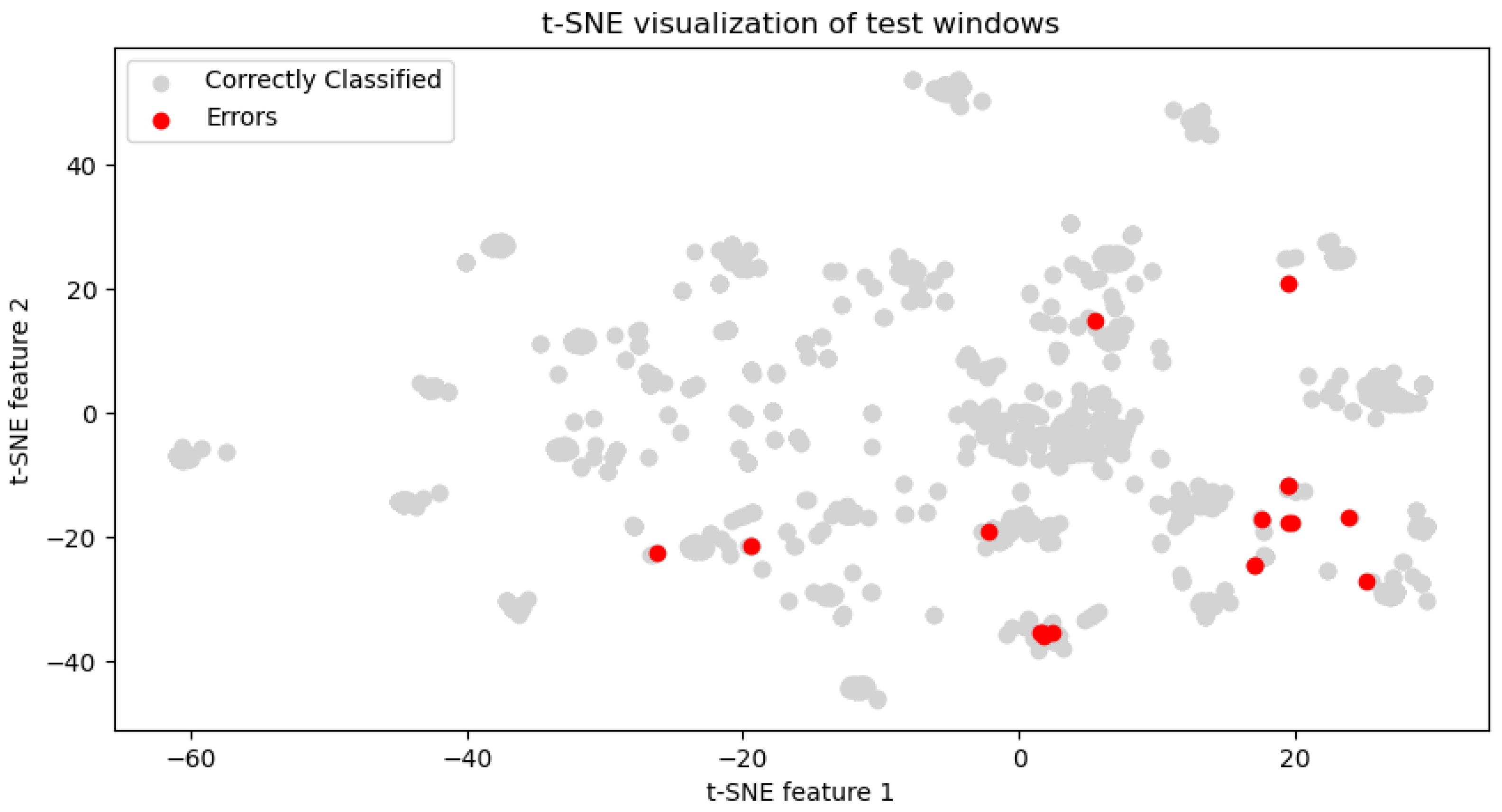
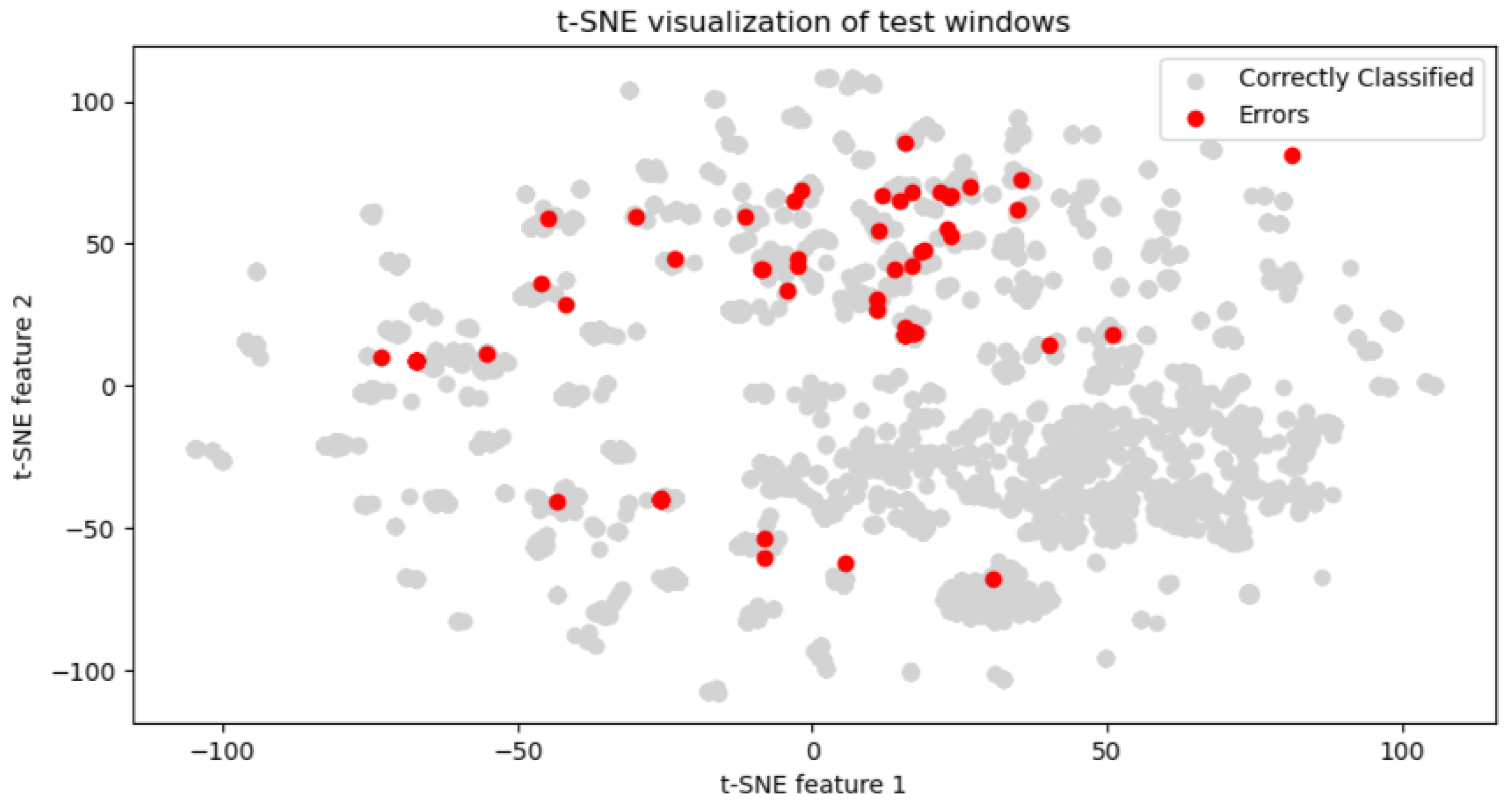
In the error-analysis phase, we utilized t-Distributed Stochastic Neighbor Embedding (t-SNE) [66], a powerful algorithm for dimensionality reduction, which is well suited to the visualization of high-dimensional datasets. Our primary goal with this analysis was to identify patterns and clusters in models’ predictions, specifically focusing on distinguishing between correctly classified instances and errors.
We transformed the test data into a two-dimensional space with t-SNE and plotted the two-dimensional features with plot points color-coded to distinguish between correctly classified instances (in light gray) and errors (in red). This visualization reveals areas where the model performs well and highlights regions where errors are concentrated.
In both t-SNE visualizations (shown in Figure 9 and Figure 10), errors, represented by red dots, are interspersed among correctly classified instances, rather than clustering in isolated areas. This pattern suggests that the errors do not stem from distinct, well-defined regions of the feature space. Instead, they appear to be spread throughout, indicating that these misclassifications are not readily separable based on the model’s current understanding of the features. This dispersion of errors points to the intrinsic difficulty of the classification task, where simple linear separability is not achievable, and more complex decision boundaries are necessary. Furthermore, we observe substantial regions within the t-SNE plots where correctly classified samples are dominant, with no errors nearby. This implies that, for a significant portion of the dataset, the model can classify instances with high confidence and accuracy. Such regions are indicative of samples that are likely easier to classify, either because they have more distinct feature representations or they fall far from the decision boundary within the feature space.
Overall, while the model showed competence in accurately classifying a large fraction of the data, the scattered errors highlight the challenges present in the more ambiguous regions of the feature space.

5.7. Ablation Study

5.7.1. The Effect of Text Representation

In this section, we assess the effect that textual feature representation has on the scores of the top models described in the previous section. We report the results these models achieved on the PARSEC-500 and PARSEC-5000 datasets with a window size of 7 when 1-hot vectors, FastText vectors, or BERT sentence embeddings were chosen to encode textual features (see Section 3.6 for details).
F1 scores, sensitivity, specificity, and test times for tests appear in Table 7. Full results for all models, dataset features, and all window sizes are available in Appendix A in Appendix A.5 and Appendix A.6.
For both the PARSEC-500 and PARSEC-5000 datasets, 1-hot encoding showed the best performance and indicated that, despite its simplicity, it is highly effective for our task. FastText appears to be the least effective among the tested representations, yielding the lowest F1 scores for both models. This might suggest that FastText’s sub-word features and simpler contextual understanding do not capture enough discriminating information for our specific dataset and task.

5.7.2. The Effect of Data Features

This section examines the top models’ performance on different feature sets, analyzed on the PARSEC-500 and PARSEC-5000 datasets (full results for additional features are available in Appendix A in Appendix A.7). Feature sets are described in Section 3.5. The results are presented in Table 8. We observed that, surprisingly, the best scores of all four models were achieved when the smaller feature set was selected (OpsRes for PARSEC-500 and Ops for PARSEC-5000). Moreover, adding process-duration features and process details reduced the sensitivity and F1 score drastically, implying that these features interfere with the abilities of neural models to detect ransomware. One possible reason is that these features introduce noise and may be correlated with existing features, leading to redundancy and diluting the impact of significant features. Additionally, increasing data dimensionality makes learning more difficult for models if the new features do not carry substantial information relevant to the task.

5.7.3. The Effect of the API Call-Window Size

This section examines top models’ performance on different API call-sequence sizes, analyzed on the PARSEC-500 dataset (full results are available in Appendix A in Appendix A.5 and Appendix A.6). We examined how the scores were affected by selecting window sizes of W = 1 , 3 , 5 , 7 . The results are presented in Table 9. Because the top models for both datasets have W = 7, we were interested in seeing how sharp the drop was in the F1 scores. We can see that the scores decreased steadily when the window size fell from 7 to 5 and 3, but the biggest decrease happened when the window size was set to 1. This is a clear indication of the need for neural models to have information on more than one consecutive system call for every process.

5.7.4. Increasing the Number of Training Epochs

This section examines the top models’ performance with different numbers of training epochs, analyzed on the PARSEC-500 and PARSEC-5000 datasets. We examined how the scores were affected by selecting the number of epochs to be ep = 10 , 20 , 30 . Table 10 shows the results of this evaluation, including test and train times. We can see that the best performance was achieved for ep = 10 and that there was no need to increase the number of training epochs beyond that. This decision decreased the training time significantly, especially for the PARSEC-500 dataset. We also observed that the test times were not affected by increasing the number of training epochs.

5.7.5. Different Train–Test Splits

Here, we present the results of our test for our top models’ robustness by applying them to different train–test splits (described in Section 4.2) to the PARSEC-500 and PARSEC-5000 datasets. In these splits, different benign and ransomware processes were assigned to the train and test sets. Table 11 shows how selecting different processes during the train–test split affects the ratio of API call features unique to benign or ransomware processes. These calls help the models identify processes without the need for deep analysis. Additionally, we found the feature SetRenameInformationFile to be a unique ransomware feature that was recorded 1111 times exclusively in ransomware activities. This feature was not present in any of the benign processes.
Table 12 contains the results of the top models on the PARSEC-500 and PARSEC-5000 datasets with different data splits. We observed that sensitivity scores remained high or identical for both datasets and for different splits, but there was variability in the F1 scores on the PARSEC-500 dataset. The high or identical sensitivity scores across different splits suggest that the models were consistently good at identifying positive cases in both datasets, which indicates the models’ robustness. The variability in F1 scores on the PARSEC-500 dataset implies that the choice of processes for the training set can significantly affect the models’ performance in terms of precision and recall balance. However, the reduced variability in F1 scores on the larger PARSEC-5000 dataset indicates that a larger dataset provides more stable and reliable performance, reducing the impact of specific training-set selections. We conclude that longer API call sequences in the PARSEC-5000 dataset led to successful ransomware detection, regardless of the training-set processes. This observation implies that more comprehensive data (longer sequences) enhance the models’ robustness and reliability. For the smaller PARSEC-500 dataset, the selection of processes for the training set had a more pronounced effect on the models’ performance. This suggests that, with limited data, the specific characteristics of the training set play a crucial role in determining the models’ effectiveness. It highlights the importance of careful training set selection in low-data scenarios.

5.7.6. The Effect of Unbalanced Data

Table 13 illustrates the behavior of a binary classification model when evaluated on test sets with varying class ratios despite being trained on a balanced dataset. Interestingly, the F1 score rose with the percentage of class 1 (the RW class) in the test data. When class 1 was underrepresented, for example, at 1% of the test set, the F1 score was lower; nevertheless, as the distribution became more balanced, at 40% of the RW class, the F1 score increased dramatically. The model reliably identified positive and negative instances with high accuracy, maintaining exceptional sensitivity and specificity across all configurations despite these differences in F1 score. The models’ fundamental capability to identify both classes was demonstrated by their consistency in sensitivity and specificity. This indicates that the core ability of our models to detect both classes remained strong, even as the class distribution in the test set shifted.

6. Conclusions

In this paper, we have explored the efficacy of deep learning techniques in the early detection of ransomware through the analysis of API call sequences. We designed and created a comprehensive dataset of initial API call sequences of popular benign processes and verified ransomware processes. We also performed a comprehensive analysis of different baseline and neural-network models applied to the task of ransomware detection on this dataset.
Our investigation has provided substantial evidence that neural network models, especially CNN and LSTM, can be effectively applied to differentiate between benign and malicious system behaviors. We demonstrated that these models outperform traditional ML classifiers (baselines) and a competing method of [29], providing a positive answer to RQ1. Our findings indicate that the inclusion of the result feature for each API call significantly improved the models’ performance, providing a positive answer to RQ2. We also found that 1-hot encoding of text features yielded the best results, answering RQ3. We, moreover, learned that increasing the number W of consecutive API calls used in the analysis improved the classification accuracy and F1-measure and that setting W = 7 was sufficient to achieve state-of-the-art results.
Across various configurations, the combination of operation and result features yielded the best results. Additionally, our analysis showed that a window size of 7 provided optimal performance, and 1-hot encoding (OH) generally outperformed other encoding methods in terms of accuracy, answering RQ4. Finally, we learned that the test times of neural models are suitable for online ransomware detection, which resolves RQ5.
We hope the PARSEC dataset will become a valuable resource for the cybersecurity community and encourage further research in the area of ransomware detection. Our findings contribute to the development of more robust and efficient ransomware detection systems, advancing the field of cybersecurity.

7. Limitations and Future Research Directions

The findings of this paper open several directions for future research, namely (1) the expansion of the dataset to capture a broader spectrum of real user activities and (2) the exploration of real-time detection systems integrated into network infrastructures. The PARSEC dataset, while robust, primarily includes API call sequences from simulated benign and ransomware processes. There is a compelling need to develop a dataset that will include activities from diverse computing environments such as office tasks, multimedia processing, software development, and gaming. Current ransomware detection models largely operate by analyzing static datasets. However, integrating these models into live network systems could facilitate the detection of ransomware as it attempts to execute. This approach would enable a more dynamic and proactive response to ransomware threats.
The limitations of our approach are the challenges associated with using API call features and neural models for ransomware detection. Collecting and labeling a comprehensive dataset of API call sequences from benign and ransomware processes is complex, time-consuming, and resource-intensive. Maintaining dataset quality and relevance as ransomware evolves requires substantial effort and depends on the chosen processes. Neural models, particularly deep learning ones, risk overfitting specific patterns in the training data. This can result in recognizing only known ransomware sequences, rather than general malicious behavior, necessitating extensive and resource-heavy testing to ensure good generalization. We also observed that the selection of processes for the training set had an effect on the performance of the model when shorter API call sequences were used as training data. This means that future applications should be mindful of this phenomenon.
Author Contributions

Conceptualization, M.K., M.D. and N.V.; methodology, M.K., M.D. and N.V.; software, M.D.; validation, M.D.; formal analysis, M.K., M.D. and N.V.; resources, M.K. and M.D.; data curation, M.D.; writing—original draft preparation, M.K. and N.V.; writing—review and editing, M.K., M.D. and N.V.; supervision, M.K. and N.V. All authors have read and agreed to the published version of the manuscript.

Funding

This research received no external funding.

Data Availability Statement

The PARSEC dataset and the code reside in a public repository on GitHub. It is freely available to the community at https://github.com/MatanDavidian/MSc–Ransomware-Detection-Using-Deep-Learning-Models.

Conflicts of Interest

The authors declare no conflicts of interest.

Abbreviations

The following abbreviations are used in this manuscript:
APIApplication programming interface
BERTBidirectional encoder representations from transformers
CNNConvolutional neural network
CPUCentral processing unit
DGCNNDeep graph convolutional neural network
DGNNDeep graph neural network
DLDeep learning
DNNDeep neural network
F1F1 measure
FPsFalse positives
FNsFalse negatives
GDDR5Graphics double data rate type five
GPUGraphics processing unit
IRPI/O request packet
kNNk-nearest neighbors
LSTMLong short-term memory
LRLogistic regression
MLMachine learning
MLPMulti-layer perceptron
NLPNatural language processing
OpsOperations
OpsResOperations with results
OpsResDurOperations with results and duration
OpsResDurDetOperations with results, duration, and details
OSOperating system
PPrecision
PMProcess monitor
RRecall
RaaSRansomware-as-a-service
RAMRandom access memory
RFRandom forest
RNNRecurrent neural network
RQResearch question
RWRansomware
SSDSolid-state drive
SVMSupport vector machine
SESentence embeddings
SP1Service Pack 1
TPsTrue positives
TNsTrue negatives
VMVirtual machine

Appendix A

Appendix A.1. Full List of Benign Processes

Table A1 lists the benign processes we used in the PARSEC dataset’s construction.
Table A1. General benign processes.
Process NameCategory
General Processes
AxCrypt.exeencryption
ffmpeg.exemultimedia
EXCEL.EXEoffice
WinRAR.execompression
WINWORD.EXEoffice
7zG.execompression
curl.exedownloading
lame.exemultimedia
benchmarking processes
PerformanceTest64.exePass Mark
PT-CPUTest64.exePass Mark
PT-BulletPhysics64.exePass Mark
soffice.binPC Mark
libreofficeCalcTest.exePC Mark
Browsing.exePC Mark
MFPlayback.exePC Mark
MFVideoChat2.exePC Mark
WordProcessing.exePC Mark
NativeApp.exePC Mark
Table A2 contains the full list of idle-state processes.
Table A2. Idle-state benign processes.
Process Names
SystemSearchIndexer.exeCobian.Reflector.UserInterface.exe
Idlesmss.execsrss.exe
wininit.exewinlogon.exeservices.exe
lsass.exelsm.exesvchost.exe
VBoxService.exeAUDIODG.EXEspoolsv.exe
taskhost.exeCobian.Reflector.VSCRequester.exetaskeng.exe
sppsvc.exeDwm.exeExplorer.EXE
VBoxTray.exeCobian.Reflector.Application.exebtweb.exe
steam.exehelper.exewmpnetwk.exe
wmiprvse.exeSearchProtocolHost.exeSearchFilterHost.exe
cmd.execonhost.exepowershell.exe
DllHost.exeWMIADAP.EXEIntelSoftwareAssetManagerService.exe
sc.exesdclt.exeDiagTrackRunner.exe
wsqmcons.exeschtasks.exeCompatTelRunner.exe
GoogleUpdate.exeGoogleCrashHandler.exeGoogleCrashHandler64.exe
DeviceDisplayObjectProvider.exesdclt.exesteam.exe
DeviceDisplayObjectProvider.exeDiagTrackRunner.exehelper.exe
GoogleCrashHandler.execompattelrunner.exeGoogleUpdate.exe

Appendix A.2. Full Information on Process Parameters

Table A3 contains the full list of process details parameters used in the PARSEC datasets.
Table A3. List of process-detail parameters.
Parameters
FileAttributesDeletePendingDispositionOptions
AttributesShareModeAccessExclusive
FailImmediatelyOpenResultPageProtectionControl
ExitStatusPrivateBytesPeakPrivateBytesWorkingSet
PeakWorkingSetCommandlinePriorityGrantedAccess
NameTypeDataQuery
HandleTagsI/OFlagsFileSystemAttributesDesiredAccess
Table A4 contains the full list of process-detail parameters filtered out from the PARSEC dataset.
Table A4. List of unused process parameters.
Parameters
PIDIDconnidChangeTime
CreationTimeLastAccessTimeLastWriteTimeStartime
EndtimeTimeVolumeCreationTimeDirectory
FileNameSizeAllocationSizeEaSize
EnvironmentFileInformationClassFileSystemNameLength
MaximumComponentNameLength
Table A5 contains the full list of process operation names used in our dataset.
Table A5. List of process operation names.
Parameters
CloseFileCreateFileCreateFileMapping
DeviceIoControlFASTIO_ACQUIRE_FOR_CC_FLUSH
FASTIO_ACQUIRE_FOR_MOD_WRITE
FASTIO_MDL_READ_COMPLETE
FASTIO_MDL_WRITE_COMPLETE
FASTIO_RELEASE_FOR_CC_FLUSH
FASTIO_RELEASE_FOR_MOD_WRITE
FASTIO_RELEASE_FOR_SECTION_SYNCHRONIZATION
FileSystemControlFlushBuffersFileIRP_MJ_CLOSE
Load ImageLockFileNotifyChangeDirectory
Process CreateProcess ExitProcess Profiling
Process StartQueryAllInformationFileQueryAttributeInformationVolume
QueryAttributeTagFileQueryBasicInformationFileQueryDirectory
QueryEaInformationFileQueryFileInternalInformationFileQueryInformationVolume
QueryNameInformationFileQueryNetworkOpenInformationFileQueryNormalizedNameInformationFile
QueryOpenQuerySecurityFileQuerySizeInformationVolume
QueryStandardInformationFileQueryStreamInformationFileReadFile
RegCloseKeyRegCreateKeyRegDeleteKey
RegDeleteValueRegEnumKeyRegEnumValue
RegLoadKeyRegOpenKeyRegQueryKey
RegQueryKeySecurityRegQueryMultipleValueKeyRegQueryValue
RegSetInfoKeyRegSetValueSetAllocationInformationFile
SetBasicInformationFileSetDispositionInformationFileSetEndOfFileInformationFile
SetRenameInformationFileSetSecurityFileTCP Accept
TCP ConnectTCP DisconnectTCP Receive
TCP SendTCP TCPCopyThread Create
Thread ExitUDP ReceiveUDP Send
UnlockFileSingleWriteFile
Table A6 contains the full list of API call-result parameters used in our dataset.
Table A6. List of API call-result parameters.
Parameters
SUCCESSFILE LOCKED WITH ONLY READERS
FILE LOCKED WITH WRITERSACCESS DENIED
IS DIRECTORYNAME COLLISION
NAME INVALIDNAME NOT FOUND
PATH NOT FOUNDREPARSE
SHARING VIOLATIONFAST IO DISALLOWED
INVALID PARAMETERCANT WAIT
END OF FILEINVALID DEVICE REQUEST
NOT REPARSE POINTNOTIFY CLEANUP
BUFFER OVERFLOWNO MORE FILES
NO SUCH FILENO MORE ENTRIES
BUFFER TOO SMALLFILE LOCK CONFLICT

Appendix A.3. The Number of System Calls for for Benign and Ransomware Processes

Table A7 and Table A8 show the total numbers for API system calls for benign and ransomware processes for the PARSEC-500 and PARSEC-5000 datasets.
Table A7. Comparison of system call amounts for the PARSEC-500 dataset.
OperationBenignRansomware
CloseFile11685052
CreateFile19215061
CreateFileMapping17740
FASTIO_ACQUIRE_FOR_CC_FLUSH1770
FASTIO_ACQUIRE_FOR_MOD_WRITE580
FASTIO_RELEASE_FOR_CC_FLUSH1760
FASTIO_RELEASE_FOR_MOD_WRITE520
FASTIO_RELEASE_FOR_SECTION_SYNCHRONIZATION15400
FileSystemControl2980
IRP_MJ_CLOSE9153717
Load Image5430
Process Create50
Process Exit40
Process Profiling6402228
Process Start340
QueryAllInformationFile60
QueryAttributeInformationVolume150
QueryAttributeTagFile5141269
QueryBasicInformationFile3273306
QueryDirectory153601
QueryFileInternalInformationFile7770
QueryInformationVolume360
QueryNameInformationFile1310
QueryNetworkOpenInformationFile960
QueryNormalizedNameInformationFile20
QueryOpen3881075
QuerySecurityFile620
QueryStandardInformationFile6781230
ReadFile16182888
RegCloseKey12780
RegCreateKey320
RegDeleteKey20
RegDeleteValue180
RegEnumKey2530
RegEnumValue770
RegOpenKey26170
RegQueryKey15460
RegQueryKeySecurity560
RegQueryMultipleValueKey80
RegQueryValue18720
RegSetInfoKey1730
RegSetValue100
SetBasicInformationFile7801123
SetEndOfFileInformationFile40
SetRenameInformationFile01259
TCP Connect10
TCP Receive80
TCP Send30
Thread Create1680
Thread Exit1320
UDP Receive50
WriteFile2162606
Table A8. Comparison of system-call amounts for the PARSEC-5000 dataset.
OperationBenignRansomware
CloseFile915122,323
CreateFile11,04423,374
CreateFileMapping78310
DeviceIoControl480
FASTIO_ACQUIRE_FOR_CC_FLUSH16340
FASTIO_ACQUIRE_FOR_MOD_WRITE7350
FASTIO_MDL_READ_COMPLETE50
FASTIO_MDL_WRITE_COMPLETE50
FASTIO_RELEASE_FOR_CC_FLUSH16340
FASTIO_RELEASE_FOR_MOD_WRITE7310
FASTIO_RELEASE_FOR_SECTION_SYNCHRONIZATION65600
FileSystemControl4660
FlushBuffersFile20
IRP_MJ_CLOSE697517,031
Load Image20590
LockFile20
NotifyChangeDirectory10
Process Create340
Process Exit380
Process Profiling8996388
Process Start560
QueryAllInformationFile4770
QueryAttributeInformationVolume2130
QueryAttributeTagFile11894645
QueryBasicInformationFile221015,182
QueryDirectory19164546
QueryEaInformationFile100
QueryFileInternalInformationFile14690
QueryInformationVolume6190
QueryNameInformationFile12890
QueryNetworkOpenInformationFile13850
QueryNormalizedNameInformationFile20
QueryOpen36366987
QuerySecurityFile5590
QuerySizeInformationVolume10
QueryStandardInformationFile24434635
QueryStreamInformationFile100
ReadFile19,00510,593
RegCloseKey13,2070
RegCreateKey3510
RegDeleteKey90
RegDeleteValue340
RegEnumKey18060
RegEnumValue8360
RegLoadKey70
RegOpenKey24,7540
RegQueryKey14,7630
RegQueryKeySecurity4520
RegQueryMultipleValueKey340
RegQueryValue24,2980
RegSetInfoKey10790
RegSetValue700
SetAllocationInformationFile20
SetBasicInformationFile14964992
SetDispositionInformationFile40
SetEndOfFileInformationFile750
SetRenameInformationFile34643
SetSecurityFile80
TCP Accept20
TCP Connect30
TCP Disconnect40
TCP Receive20220
TCP Send70
TCP TCPCopy50
Thread Create4730
Thread Exit3430
UDP Receive410
UDP Send190
UnlockFileSingle20
WriteFile52519986

Appendix A.4. Operations’ Visualization for Benign and Ransomware Processes

Figure A1, Figure A2, Figure A3, Figure A4 and Figure A5 show the distribution of operational API calls for various benign processes.
Figure A1. AxCrypt.exe (encryption tool).
Futureinternet 16 00291 g0a1
Figure A2. WinRAR.exe (file compression and archiving).
Futureinternet 16 00291 g0a2
Figure A3. lame.exe (audio encoder).
Futureinternet 16 00291 g0a3
Figure A4. Explorer.EXE (file management and navigation).
Futureinternet 16 00291 g0a4
Figure A5. GoogleCrashHandler.exe (crash reporting service).
Futureinternet 16 00291 g0a5
Figure A6, Figure A7, Figure A8, Figure A9 and Figure A10 show the distribution of operational API calls for various ransomware process types.
Figure A6. 3359dff8c8b3855e8cf980539e7fb300.exe (ransomware sample).
Futureinternet 16 00291 g0a6
Figure A7. 0b7fa305b57066885d7d70c96d51aae0.exe (ransomware sample).
Futureinternet 16 00291 g0a7
Figure A8. 1a4bf948ba5876657cde4ea846e13f74.exe (ransomware sample).
Futureinternet 16 00291 g0a8
Figure A9. 6e20f33646814a547b1d6a9b55343e38.exe (ransomware sample).
Futureinternet 16 00291 g0a9
Figure A10. 66b7a800f6a7f327de0eed42407074ce.exe (ransomware sample).
Futureinternet 16 00291 g0a10

Appendix A.5. Full Experimental Results for the MLP Model

Table A9 and Table A10 contain full evaluation results for the MLP model on the PARSEC-500 and PARSEC-5000 datasets. This evaluation shows all feature combinations (Ops, OpsRes, OpsResDur, and OpsResDurDet), all text representations (1-hot encoding, FastText word vectors, and BERT sentence embeddings), and all window sizes (1, 3, 5, and 7). We report sensitivity, specificity, and F1 measures for every data setup. Note that, for the two large feature sets, 1-hot results are not reported because the vectors were too large for the model to be trained within a reasonable amount of time. The data reveal a pattern of increasing scores for all the datasets with the best results achieved for W = 7. There was a significant boost in performance when the sequence size was increased from 1 to 3, and further increases in sequence size yielded progressively smaller improvements. The test time remained small, and its variations suggest that, while larger window sizes typically increase the computational time, the effect is not uniformly significant across all API call amounts.
Table A9. Full experimental results for the MLP model on the PARSEC-500 dataset.
ModelText reprFLISTSensitivitySpecificityF1W
MLP1-hotOp0.99230.66820.85390.011
MLP1-hotOp0.99540.89530.94790.003
MLP1-hotOp0.99770.91690.95900.005
MLP1-hotOp0.99670.94580.97200.007
MLPBERT SEOp0.99290.66910.85460.041
MLPBERT SEOp0.99580.89340.94730.033
MLPBERT SEOp0.99690.89460.94840.035
MLPBERT SEOp0.99350.96640.98020.037
MLPFastTextOp0.90860.54740.76960.021
MLPFastTextOp0.96340.69510.84940.023
MLPFastTextOp0.92230.82380.87900.025
MLPFastTextOp0.94800.77790.87370.017
MLP1-hotOpRes0.98850.70170.86450.011
MLP1-hotOpRes0.99580.89940.95000.013
MLP1-hotOpRes0.99690.93460.96680.005
MLP1-hotOpRes0.99460.95670.97610.007
MLPBERT SEOpRes0.98920.68370.85810.081
MLPBERT SEOpRes0.99490.86010.93210.073
MLPBERT SEOpRes0.99770.89540.94910.075
MLPBERT SEOpRes0.99670.93720.96790.137
MLPFastTextOpRes0.94550.59940.80600.101
MLPFastTextOpRes0.97130.75020.87460.033
MLPFastTextOpRes0.97150.82920.90700.035
MLPFastTextOpRes0.93170.86460.90150.037
MLPBERT SEOpResDur0.98920.68580.85890.091
MLPBERT SEOpResDur0.99210.87030.93510.183
MLPBERT SEOpResDur1.00000.89310.94930.195
MLPBERT SEOpResDur0.98050.93720.95970.097
MLPFastTextOpResDur0.94720.59880.80670.051
MLPFastTextOpResDur0.96850.77900.88470.043
MLPFastTextOpResDur0.97920.79770.89770.035
MLPFastTextOpResDur0.96530.82340.90140.037
MLPBERT SEOpResDurDet0.98510.72120.87030.471
MLPBERT SEOpResDurDet0.99720.88000.94200.483
MLPBERT SEOpResDurDet0.98230.91230.94910.485
MLPBERT SEOpResDurDet0.98270.93170.95830.477
MLPFastTextOpResDurDet0.94090.64380.81920.201
MLPFastTextOpResDurDet0.98560.84990.92300.213
MLPFastTextOpResDurDet0.98920.88080.93830.185
MLPFastTextOpResDurDet0.96530.92960.94840.187
Table A10. Full experimental results for the MLP model on the PARSEC-5000 dataset.
ModelText reprFLISTSensitivitySpecificityF1W
MLP1-hotOp0.99570.67410.85780.181
MLP1-hotOp0.99740.89470.94870.053
MLP1-hotOp0.99990.94790.97460.045
MLP1-hotOp0.99890.98010.98960.047
MLPBERT SEOp0.99520.67690.858611.021
MLPBERT SEOp0.99790.88430.94430.313
MLPBERT SEOp0.99900.95300.97650.405
MLPBERT SEOp0.99950.96680.98340.347
MLPFastTextOp0.87320.63540.78043.671
MLPFastTextOp0.98500.81790.90900.143
MLPFastTextOp0.98280.88890.93880.155
MLPFastTextOp0.99150.89910.94770.137
MLP1-hotOpRes0.98820.71030.86760.191
MLP1-hotOpRes0.99880.92050.96120.073
MLP1-hotOpRes0.99970.95380.97730.065
MLP1-hotOpRes0.99990.98490.99250.057
MLPFastTextOpRes0.98880.63860.84152.531
MLPFastTextOpRes0.99190.79210.90180.243
MLPFastTextOpRes0.98370.91180.94950.235
MLPFastTextOpRes0.99060.94460.96840.257
MLPFastTextOpResDur0.98640.63490.83902.611
MLPFastTextOpResDur0.99640.77950.89890.373
MLPFastTextOpResDur0.97930.91110.94700.355
MLPFastTextOpResDur0.95830.94900.95390.387

Appendix A.6. Full Experimental Results for Neural Models

Table A11 and Table A12 contain full evaluation results for the neural models (DNN, CNN, and LSTM) on the PARSEC-500 and PARSEC-5000 datasets. This evaluation shows all feature combinations, all text representations, and all window sizes. We report sensitivity, specificity, and F1 measures for every data setup.
Table A11. Full experimental results of neural models on the PARSEC-500 dataset.
ModelText reprFLISTSensitivitySpecificityF1W
DNNBERT SEOps0.99290.66150.85181
DNNBERT SEOps0.99810.88600.94523
DNNBERT SEOps1.00000.84310.92725
DNNBERT SEOps0.98590.95670.97177
DNNFastTextOps0.99280.48280.79111
DNNFastTextOps0.98190.73400.87363
DNNFastTextOps0.96380.83230.90445
DNNFastTextOps0.94260.89490.92067
DNN1-hotOps0.99230.66820.85391
DNN1-hotOps0.99540.87260.93783
DNN1-hotOps0.99770.93310.96655
DNN1-hotOps0.99350.94370.96937
DNNBERT SEOpsRes0.98920.67910.85641
DNNBERT SEOpsRes0.98380.85820.92573
DNNBERT SEOpsRes0.99690.88770.94535
DNNBERT SEOpsRes0.99780.92200.96147
DNNFastTextOpsRes0.90620.62120.79321
DNNFastTextOpsRes0.88280.86050.87313
DNNFastTextOpsRes0.97310.85230.91775
DNNFastTextOpsRes0.95670.89170.92657
DNN1-hotOpsRes0.98850.70170.86451
DNN1-hotOpsRes0.99490.90220.95083
DNN1-hotOpsRes1.00000.93150.96695
DNN1-hotOpsRes0.99670.95990.97877
DNNBERT SEOpsResDur0.98920.68520.85871
DNNBERT SEOpsResDur0.99910.84620.92813
DNNBERT SEOpsResDur0.99230.89690.94715
DNNBERT SEOpsResDur0.99130.92850.96117
DNNFastTextOpsResDur0.98970.64450.84401
DNNFastTextOpsResDur0.92860.81370.87823
DNNFastTextOpsResDur0.96850.86920.92275
DNNFastTextOpsResDur0.96320.89380.93097
DNNBERT SEOpsResDurDet0.98510.72120.87031
DNNBERT SEOpsResDurDet0.99810.87860.94183
DNNBERT SEOpsResDurDet0.99460.91150.95495
DNNBERT SEOpsResDurDet0.96860.95340.96137
DNNFastTextOpsResDurDet0.97880.68510.85341
DNNFastTextOpsResDurDet0.98750.86330.92983
DNNFastTextOpsResDurDet0.98230.90380.94525
DNNFastTextOpsResDurDet0.97290.93390.95437
CNNBERT SEOps0.99290.66910.85461
CNNBERT SEOps0.99810.86610.93633
CNNBERT SEOps0.99540.90850.95395
CNNBERT SEOps0.98590.96530.97597
CNNFastTextOps0.99280.52820.80561
CNNFastTextOps0.96900.73350.86693
CNNFastTextOps0.96000.86770.91765
CNNFastTextOps0.95990.86570.91677
CNN1-hotOps0.99230.66820.85391
CNN1-hotOps0.99910.86890.93803
CNN1-hotOps0.99620.91770.95855
CNN1-hotOps0.99890.94370.97217
CNNBERT SEOpsRes0.98920.67910.85641
CNNBERT SEOpsRes0.99300.86380.93283
CNNBERT SEOpsRes0.99850.89690.95025
CNNBERT SEOpsRes0.99890.92960.96547
CNNFastTextOpsRes0.98910.58370.82241
CNNFastTextOpsRes0.99300.78590.89993
CNNFastTextOpsRes0.98080.86310.92635
CNNFastTextOpsRes0.96100.87870.92307
CNN1-hotOpsRes0.98850.70170.86451
CNN1-hotOpsRes0.99630.91010.95513
CNN1-hotOpsRes0.99620.94310.97045
CNN1-hotOpsRes0.99780.98270.99037
CNNBERT SEOpsResDur0.98920.68580.85891
CNNBERT SEOpsResDur0.99950.81650.91573
CNNBERT SEOpsResDur0.96150.91080.93775
CNNBERT SEOpsResDur0.98810.93820.96417
CNNFastTextOpsResDur0.98620.58450.82121
CNNFastTextOpsResDur0.98010.78780.89413
CNNFastTextOpsResDur0.97080.87620.92695
CNNFastTextOpsResDur0.97070.87430.92617
CNNBERT SEOpsResDurDet0.98400.72140.86981
CNNBERT SEOpsResDurDet0.99770.88370.94393
CNNBERT SEOpsResDurDet0.99690.91080.95585
CNNBERT SEOpsResDurDet0.99780.93070.96547
CNNFastTextOpsResDurDet0.94050.64230.81841
CNNFastTextOpsResDurDet0.99030.84150.92173
CNNFastTextOpsResDurDet0.90150.92310.91145
CNNFastTextOpsResDurDet0.97290.89170.93497
LSTMBERT SEOps0.99290.66910.85461
LSTMBERT SEOps0.99720.85870.93263
LSTMBERT SEOps0.99620.91540.95755
LSTMBERT SEOps0.99780.94470.97207
LSTMFastTextOps0.94860.60420.80921
LSTMFastTextOps0.98150.75900.88323
LSTMFastTextOps0.98380.79150.89755
LSTMFastTextOps0.96530.84400.91017
LSTM1-hotOps0.99230.66820.85391
LSTM1-hotOps0.98930.86240.93033
LSTM1-hotOps0.99770.91230.95685
LSTM1-hotOps0.99570.94260.96997
LSTMBERT SEOpsRes0.98920.68370.85811
LSTMBERT SEOpsRes0.99440.86050.93203
LSTMBERT SEOpsRes0.99920.90460.95415
LSTMBERT SEOpsRes0.99350.93390.96487
LSTMFastTextOpsRes0.98910.64680.84451
LSTMFastTextOpsRes0.94350.85400.90313
LSTMFastTextOpsRes0.97380.87920.92995
LSTMFastTextOpsRes0.96320.90470.93587
LSTM1-hotOpsRes0.98850.70170.86451
LSTM1-hotOpsRes0.99070.86750.93323
LSTM1-hotOpsRes1.00000.91460.95915
LSTM1-hotOpsRes1.00000.97510.98777
LSTMBERT SEOpsResDur0.98920.68580.85891
LSTMBERT SEOpsResDur0.98610.85360.92483
LSTMBERT SEOpsResDur0.99920.90230.95305
LSTMBERT SEOpsResDur0.99780.93500.96747
LSTMFastTextOpsResDur0.98940.64450.84391
LSTMFastTextOpsResDur0.93000.84150.89063
LSTMFastTextOpsResDur0.98540.87150.93235
LSTMFastTextOpsResDur0.96860.89270.93327
LSTMBERT SEOpsResDurDet0.98510.72120.87031
LSTMBERT SEOpsResDurDet0.99720.89480.94863
LSTMBERT SEOpsResDurDet0.99540.92310.96075
LSTMBERT SEOpsResDurDet0.99240.94040.96737
LSTMFastTextOpsResDurDet0.90170.71850.82601
LSTMFastTextOpsResDurDet0.99170.87490.93703
LSTMFastTextOpsResDurDet0.97690.90690.94395
LSTMFastTextOpsResDurDet0.97290.92310.94937
Table A12. Full experimental results of neural models on the PARSEC-5000 dataset.
ModelText reprFLISTSensitivitySpecificityF1W
DNN1-hotOp0.99570.67460.8581
DNN1-hotOp0.99810.89480.94943
DNN1-hotOp0.99930.96100.98085
DNN1-hotOp0.99920.97790.98907
DNNBERT SEOp0.99520.67730.86761
DNNBERT SEOp0.99800.89730.95313
DNNBERT SEOp0.99980.95290.97735
DNNBERT SEOp0.99980.95090.97607
DNNFastTextOp0.99560.63340.85001
DNNFastTextOp0.99290.81000.91293
DNNFastTextOp0.97870.88780.93645
DNNFastTextOp0.94820.93040.94437
DNN1-hotOpRes0.98820.71040.87981
DNN1-hotOpRes0.99900.90880.95933
DNN1-hotOpRes0.99990.96260.98235
DNN1-hotOpRes0.99970.98700.99427
DNNFastTextOpRes0.99390.60480.83311
DNNFastTextOpRes0.96550.78800.89613
DNNFastTextOpRes0.98940.91720.95565
DNNFastTextOpRes0.98290.93370.96067
DNNFastTextOpResDur0.99060.61230.83901
DNNFastTextOpResDur0.99410.79100.90273
DNNFastTextOpResDur0.99520.89670.94875
DNNFastTextOpResDur0.98560.92100.95497
CNN1-hotOp0.99570.67470.85861
CNN1-hotOp0.99830.89380.94883
CNN1-hotOp0.99980.95730.98055
CNN1-hotOp0.99880.97290.98877
CNNBERT SEOp0.99520.67730.85871
CNNBERT SEOp0.99500.89770.94913
CNNBERT SEOp0.99880.95080.97595
CNNBERT SEOp0.99880.97900.98967
CNNFastTextOp0.93840.59380.81081
CNNFastTextOp0.99440.77500.89893
CNNFastTextOp0.95640.91380.93885
CNNFastTextOp0.98360.90250.94627
CNN1-hotOpRes0.98820.71030.86771
CNN1-hotOpRes0.99590.92230.96123
CNN1-hotOpRes0.99950.96450.98325
CNN1-hotOpRes0.99720.98900.99347
CNNFastTextOpRes0.98880.64020.84291
CNNFastTextOpRes0.94170.80330.88683
CNNFastTextOpRes0.98450.87180.93615
CNNFastTextOpRes0.97030.96300.96847
CNNFastTextOpResDur0.99480.63000.84151
CNNFastTextOpResDur0.99330.79260.90903
CNNFastTextOpResDur0.99570.89120.94705
CNNFastTextOpResDur0.99780.94090.97467
LSTM1-hotOp0.99570.67410.85801
LSTM1-hotOp0.99710.89440.94853
LSTM1-hotOp0.99970.96280.98165
LSTM1-hotOp0.99980.98850.99407
LSTMBERT SEOp0.99520.67720.85871
LSTMBERT SEOp0.99730.89630.94953
LSTMBERT SEOp0.99970.95110.97655
LSTMBERT SEOp0.99880.96700.98347
LSTMFastTextOp0.99560.56180.83201
LSTMFastTextOp0.93600.80820.88083
LSTMFastTextOp0.99440.90770.95395
LSTMFastTextOp0.99210.92360.95937
LSTM1-hotOpRes0.98820.71030.86761
LSTM1-hotOpRes0.99860.92250.96683
LSTM1-hotOpRes0.99970.96110.98165
LSTM1-hotOpRes1.00000.98570.99317
LSTMFastTextOpRes0.98880.66220.85781
LSTMFastTextOpRes0.99440.81590.92153
LSTMFastTextOpRes0.99650.91880.95935
LSTMFastTextOpRes0.99070.98000.98607
LSTMFastTextOpResDur0.98950.63320.84131
LSTMFastTextOpResDur0.99620.83410.93193
LSTMFastTextOpResDur0.99800.90920.95595
LSTMFastTextOpResDur0.99360.94190.97027

Appendix A.7. Full Experimental Results for Neural Models—Additional Features

Table A13 shows the results of the neural-model evaluation for the feature sets OpsResDur and OpsResDurDet on the PARSEC-5000 and PARSEC-5000 datasets.
Table A13. Full experimental results of neural models on the PARSEC-5000 and PARSEC-5000 datasets with additional process features.
PARSEC-500 dataset
modeltext reprFLISTsensitivityspecificityF1Wep
CNN1-hotOpsResDur0.61000.58180.6015710
DNN1-hotOpsResDur0.20800.94580.3296710
LSTM1-hotOpsResDur0.40850.83320.5186710
MLP1-hotOpsResDur0.01950.99890.0382710
PARSEC-5000 dataset
modeltext reprFLISTsensitivityspecificityF1Wep
CNN1-hotOpsResDurDet0.11270.98590.2000710
DNN1-hotOpsResDurDet0.05740.99570.1082710
LSTM1-hotOpsResDurDet0.11270.91220.1877710
MLP1-hotOpsResDurDet0.01840.99890.0361710

References

  1. Cloudflare Inc. (n.d.) Cloudflare. What Is Ransomware? 2024. Available online: https://www.cloudflare.com (accessed on 1 August 2024).
  2. CrowdStrike. 2024 Global Threat Report. 2024. Available online: https://www.crowdstrike.com (accessed on 1 August 2024).
  3. Urooj, U.; Al-rimy, B.A.S.; Zainal, A.; Ghaleb, F.A.; Rassam, M.A. Ransomware detection using the dynamic analysis and machine learning: A survey and research directions. Appl. Sci. 2021, 12, 172. [Google Scholar] [CrossRef]
  4. Morgan, S. Ransomware deployment methods and analysis: Views from a predictive model and human responses. Crime Sci. J. 2021, 10, 2. [Google Scholar]
  5. Herrera Silva, J.A.; Barona López, L.I.; Valdivieso Caraguay, Á.L.; Hernández-Álvarez, M. A survey on situational awareness of ransomware attacks—Detection and prevention parameters. Remote Sens. 2019, 11, 1168. [Google Scholar] [CrossRef]
  6. McDonald, G.; Papadopoulos, P.; Pitropakis, N.; Ahmad, J.; Buchanan, W.J. Ransomware: Analysing the impact on Windows active directory domain services. Sensors 2022, 22, 953. [Google Scholar] [CrossRef]
  7. Zimba, A.; Chishimba, M. Analyzing the Impact of Ransomware Attacks Globally. J. Cybersecur. Digit. Forensics 2019, 11, 26. [Google Scholar]
  8. Zimba, A.; Chishimba, M. On the economic impact of crypto-ransomware attacks: The state of the art on enterprise systems. Eur. J. Secur. Res. 2019, 4, 3–31. [Google Scholar] [CrossRef]
  9. Qartah, M.A. Ransomware Economics: Analysis of the Global Impact of Ransom Demands. J. Inf. Secur. 2020. [Google Scholar]
  10. Klick, J.; Koch, R.; Br, stetter, T. Epidemic? The attack surface of German hospitals during the COVID-19 pandemic. In Proceedings of the 2021 13th International Conference on Cyber Conflict (CyCon), Tallinn, Estonia, 25–28 May 2021; pp. 73–94. [Google Scholar]
  11. Alraizza, A.; Algarni, A. Ransomware detection using machine learning: A survey. Big Data Cogn. Comput. 2023, 7, 143. [Google Scholar] [CrossRef]
  12. Kapoor, A.; Gupta, A.; Gupta, R.; Tanwar, S.; Sharma, G.; Davidson, I.E. Ransomware detection, avoidance, and mitigation scheme: A review and future directions. Sustainability 2021, 14, 8. [Google Scholar] [CrossRef]
  13. Alzubaidi, L.; Bai, J.; Al-Sabaawi, A.; Santamaría, J.; Albahri, A.S.; Al-dabbagh, B.S.N.; Fadhel, M.A.; Manoufali, M.; Zhang, J.; Al-Timemy, A.H.; et al. A survey on deep learning tools dealing with data scarcity: Definitions, challenges, solutions, tips, and applications. J. Big Data 2023, 10, 46. [Google Scholar] [CrossRef]
  14. Shen, L.; Sun, Y.; Yu, Z.; Ding, L.; Tian, X.; Tao, D. On efficient training of large-scale deep learning models: A literature review. arXiv 2023, arXiv:2304.03589. [Google Scholar]
  15. Inc, S.C.I. Mutation Effect of Babuk Code Leakage: New Ransomware Variants. SOCRadar 2023. Available online: https://socradar.io/mutation-effect-of-babuk-code-leakage-new-ransomware-variants/ (accessed on 27 April 2024).
  16. What Is Signature-Based detection? Understanding Antivirus Signature Detection. Available online: https://riskxchange.co/1006984/what-is-signature-based-malware-detection/ (accessed on 27 April 2024).
  17. Sophos. What Are Signatures and How Does Signature-Based Detection Work? 2020. Available online: https://home.sophos.com/en-us/security-news/2020/what-is-a-signature (accessed on 27 April 2024).
  18. Odii, J.; Hampo, J.; Nigeria, O.; FO, N.; Onwuama, T. Comparative Analysis of Malware Detection Techniques Using Signature, Behaviour and Heuristics. Int. J. Comput. Sci. Inf. Secur. IJCSIS 2019, 17, 33–50. [Google Scholar]
  19. Mills, A.; Legg, P. Investigating anti-evasion malware triggers using automated sandbox reconfiguration techniques. J. Cybersecur. Priv. 2020, 1, 19–39. [Google Scholar] [CrossRef]
  20. Gómez-Hernández, J.A.; García-Teodoro, P. Lightweight Crypto-Ransomware Detection in Android Based on Reactive Honeyfile Monitoring. Sensors 2024, 24, 2679. [Google Scholar] [CrossRef]
  21. Dilhara, B.A.S. Classification of Malware using Machine learning and Deep learning Techniques. Int. J. Comput. Appl. 2021, 183, 12–17. [Google Scholar] [CrossRef]
  22. Do, N.Q.; Selamat, A.; Krejcar, O.; Herrera-Viedma, E.; Fujita, H. Deep Learning for Phishing Detection: Taxonomy, Current Challenges and Future Directions. IEEE Access 2022, 10, 36429–36463. [Google Scholar] [CrossRef]
  23. Voulkidis, A.; Skias, D.; Tsekeridou, S.; Zahariadis, T. Network Traffic Anomaly Detection via Deep Learning. Information 2021, 12, 215. [Google Scholar] [CrossRef]
  24. Tobiyama, S.; Yamaguchi, Y.; Shimada, H.; Ikuse, T.; Yagi, T. Malware Detection with Deep Neural Network Using Process Behavior. In Proceedings of the IEEE 40th Annual Computer Software and Applications Conference (COMPSAC), Atlanta, GA, USA, 10–16 June 2016; Volume 2, pp. 577–582. [Google Scholar]
  25. Alqahtani, A.; Sheldon, F.T. A survey of crypto ransomware attack detection methodologies: An evolving outlook. Sensors 2022, 22, 1837. [Google Scholar] [CrossRef]
  26. Nguyen, D.T.; Lee, S. LightGBM-based Ransomware Detection using API Call Sequences. Int. J. Adv. Comput. Sci. Appl. IJACSA 2021, 12, 138–146. [Google Scholar] [CrossRef]
  27. Lin, T.L.; Chang, H.Y.; Chiang, Y.Y.; Lin, S.C.; Yang, T.Y.; Zhuang, C.J.; Zhang, B.H. Ransomware Detection by Distinguishing API Call Sequences through LSTM and BERT Models. Comput. J. 2024, 67, 632–641. [Google Scholar] [CrossRef]
  28. Mikolov, T.; Chen, K.; Corrado, G.; Dean, J. Efficient estimation of word representations in vector space. In Proceedings of the International Conference on Learning Representations (ICLR 2013), Scottsdale, AZ, USA, 2–4 May 2013. [Google Scholar]
  29. de Oliveira, A.S.; Sassi, R.J. Behavioral Malware Detection Using Deep Graph Convolutional Neural Networks. Authorea Prepr. 2023. Available online: https://www.authorea.com/users/660121/articles/675292-behavioral-malware-detection-using-deep-graph-convolutional-neural-networks (accessed on 27 April 2024). [CrossRef]
  30. Zhang, S.; Tong, H.; Xu, J.; Maciejewski, R. Graph convolutional networks: A comprehensive review. Comput. Soc. Netw. 2019, 6, 11. [Google Scholar] [CrossRef] [PubMed]
  31. Karanam, S. Ransomware Detection Using Windows API Calls and Machine Learning. Ph.D. Thesis, Virginia Tech, Blacksburg, VA, USA, 2023. [Google Scholar]
  32. Cover, T.; Hart, P. Nearest neighbor pattern classification. IEEE Trans. Inf. Theory 1967, 13, 21–27. [Google Scholar] [CrossRef]
  33. Breiman, L. Random forests. Mach. Learn. 2001, 45, 5–32. [Google Scholar] [CrossRef]
  34. Steinwart, I.; Christmann, A. Support Vector Machines; Springer Science & Business Media: New York, NY, USA, 2008. [Google Scholar]
  35. Wright, R.E. Logistic Regression. In Reading and Understanding Multivariate Statistics; Grimm, L.G., Yarnold, P.R., Eds.; American Psychological Association: Washington, DC, USA, 1995; pp. 217–244. [Google Scholar]
  36. Maniriho, P.; Mahmood, A.N.; Chowdhury, M.J.M. API-MalDetect: Automated malware detection framework for windows based on API calls and deep learning techniques. J. Netw. Comput. Appl. 2023, 218, 103704. [Google Scholar] [CrossRef]
  37. Catak, F.O.; Yazı, A.F.; Elezaj, O.; Ahmed, J. Deep learning based Sequential model for malware analysis using Windows exe API Calls. PeerJ Comput. Sci. 2020, 6, e285. [Google Scholar] [CrossRef] [PubMed]
  38. Alibaba Cloud Malware Detection Based on Behaviors. 2024. Available online: https://tianchi.aliyun.com/competition/entrance/231694/information?lang=en-us (accessed on 12 July 2024).
  39. Almousa, M.; Basavaraju, S.; Anwar, M. Api-based ransomware detection using machine learning-based threat detection models. In Proceedings of the 2021 18th International Conference on Privacy, Security and Trust (PST), Auckland, New Zealand, 12–15 December 2021; pp. 1–7. [Google Scholar]
  40. Security, H. Windows 7 End of Support: What Does It Mean for Your Organization? 2022. Available online: https://heimdalsecurity.com/blog/windows-7-end-of-support/ (accessed on 11 May 2024).
  41. Microsoft Corporation. Process Monitor v3.61. 2023. Available online: https://techcommunity.microsoft.com/t5/sysinternals-blog/sysmon-v13-00-process-monitor-v3-61-and-psexec-v2-21/ba-p/2048379 (accessed on 24 June 2024).
  42. Oracle Corporation. Oracle VM VirtualBox. 2023. Available online: https://www.virtualbox.org/ (accessed on 24 June 2024).
  43. Russinovich, M.; Solomon, D.; Ionescu, A. Windows Internals, Part 1: Covering Windows Server 2008 R2 and Windows 7; Microsoft Press: Redmond, WA, USA, 2009. [Google Scholar]
  44. Aurangzeb, S.; Aleem, M.; Iqbal, M.A.; Islam, M.A. Ransomware: A survey and trends. J. Inf. Assur. Secur. 2017, 6, 48–58. [Google Scholar]
  45. Check Point Software Technologies. Different Types of Ransomware. 2024. Available online: https://www.checkpoint.com/cyber-hub/threat-prevention/ransomware/different-types-of-ransomware/ (accessed on 30 July 2024).
  46. VirusShare.com. Available online: https://virusshare.com/ (accessed on 25 June 2024).
  47. Gómez-Hernández, J.; Álvarez González, L.; García-Teodoro, P. R-locker: Thwarting ransomware action through a honeyfile-based approach. Comput. Secur. 2018, 73, 389–398. [Google Scholar] [CrossRef]
  48. Grave, E.; Bojanowski, P.; Gupta, P.; Joulin, A.; Mikolov, T. FastText Word Vectors. 2018. Available online: https://fasttext.cc/docs/en/crawl-vectors.html (accessed on 30 July 2024).
  49. Devlin, J.; Chang, M.W.; Lee, K.; Toutanova, K. BERT: Pre-training of Deep Bidirectional Transformers for Language Understanding. arXiv 2018, arXiv:1810.04805. [Google Scholar]
  50. Glorot, X.; Bordes, A.; Bengio, Y. Deep Sparse Rectifier Neural Networks. In Proceedings of the Fourteenth International Conference on Artificial Intelligence and Statistics (AISTATS), Fort Lauderdale, FL, USA, 11–13 April 2011; pp. 315–323. [Google Scholar]
  51. Rumelhart, D.E.; Hinton, G.E.; Williams, R.J. Learning representations by back-propagating errors. Nature 1986, 323, 533–536. [Google Scholar] [CrossRef]
  52. LeCun, Y.; Bottou, L.; Bengio, Y.; Haffner, P. Gradient-Based Learning Applied to Document Recognition. Proc. IEEE 1998, 86, 2278–2324. [Google Scholar] [CrossRef]
  53. Hochreiter, S.; Schmidhuber, J. Long short-term memory. Neural Comput. 1997, 9, 1735–1780. [Google Scholar] [CrossRef]
  54. Microsoft Corporation. Microsoft Windows 10 Enterprise Edition; Microsoft Corporation: Redmond, WA, USA, 2015. [Google Scholar]
  55. Chollet, F. Deep Learning with Python; Manning Publications Co.: New York, NY, USA, 2018; ISBN 9781617294433. [Google Scholar]
  56. Pedregosa, F.; Varoquaux, G.; Gramfort, A.; Michel, V.; Thirion, B.; Grisel, O.; Blondel, M.; Prettenhofer, P.; Weiss, R.; Dubourg, V.; et al. Scikit-learn: Machine Learning in Python. J. Mach. Learn. Res. 2011, 12, 2825–2830. [Google Scholar]
  57. Virtanen, P.; Gommers, R.; Oliphant, T.E.; Haberland, M.; Reddy, T.; Cournapeau, D.; Burovski, E.; Peterson, P.; Weckesser, W.; Bright, J.; et al. SciPy 1.0: Fundamental Algorithms for Scientific Computing in Python. Nat. Methods 2020, 17, 261–272. [Google Scholar] [CrossRef]
  58. Hunter, J.D. Matplotlib: A 2D Graphics Environment. Comput. Sci. Eng. 2007, 9, 90–95. [Google Scholar] [CrossRef]
  59. Hastie, T.; Tibshirani, R.; Friedman, J. The Elements of Statistical Learning; Springer: Cham, Switzerland, 2009. [Google Scholar]
  60. Fawcett, T. An Introduction to ROC Analysis. Pattern Recognit. Lett. 2006, 27, 861–874. [Google Scholar] [CrossRef]
  61. Powers, D.M.W. Evaluation: From Precision, Recall and F-Factor to ROC, Informedness, Markedness & Correlation. J. Mach. Learn. Technol. 2011, 2, 37–63. [Google Scholar]
  62. Rey, D.; Neuhäuser, M. Wilcoxon-Signed-Rank Test. In International Encyclopedia of Statistical Science; Lovric, M., Ed.; Springer: Berlin/Heidelberg, Germany, 2011. [Google Scholar] [CrossRef]
  63. Gulmez, S.; Kakisim, A.G.; Sogukpinar, I. XRan: Explainable deep learning-based ransomware detection using dynamic analysis. Comput. Secur. 2024, 139, 103703. [Google Scholar] [CrossRef]
  64. Maniath, S.; Ashok, A.; Poornachandran, P.; Sujadevi, V.; Au, P.S.; Jan, S. Deep learning LSTM based ransomware detection. In Proceedings of the 2017 Recent Developments in Control, Automation & Power Engineering (RDCAPE), Noida, India, 26–27 October 2017; pp. 442–446. [Google Scholar]
  65. Masum, M.; Faruk, M.J.H.; Shahriar, H.; Qian, K.; Lo, D.; Adnan, M.I. Ransomware classification and detection with machine learning algorithms. In Proceedings of the 2022 IEEE 12th Annual Computing and Communication Workshop and Conference (CCWC), Virtual, 26–29 January 2022; pp. 316–322. [Google Scholar]
  66. van der Maaten, L.; Hinton, G. Visualizing Data using t-SNE. J. Mach. Learn. Res. 2008, 9, 2579–2605. [Google Scholar]
Figure 1. Data collection pipeline.
Futureinternet 16 00291 g001
Figure 2. Ransomware verification pipeline.
Futureinternet 16 00291 g002
Figure 3. Data representation pipeline.
Futureinternet 16 00291 g003
Figure 4. curl.exe v7.71.1 (downloading software).
Futureinternet 16 00291 g004
Figure 5. 0a85ea7926dbb0ea07c702d6894ca1d0.exe (ransomware sample).
Futureinternet 16 00291 g005
Figure 6. 0adf953605c610880f4095b3b33ea2d9.exe (ransomware sample).
Futureinternet 16 00291 g006
Figure 7. 7a2a1fdc535f9b9a76443231e3f8b0c4.exe (ransomware sample).
Futureinternet 16 00291 g007
Figure 8. Ransomware detection pipeline.
Futureinternet 16 00291 g008
Figure 9. Error analysis—PARSEC-500 dataset with the top model (CNN 1-hot OpsRes W = 7 10 eps).
Futureinternet 16 00291 g009
Figure 10. Error analysis—PARSEC-5000 dataset with the top model (LSTM 1-hot Ops W = 7 10 eps).
Futureinternet 16 00291 g010
Table 1. Number of system calls comparison.
OperationPARSEC-500PARSEC-5000
BenignRansomwareBenignRansomware
CloseFile11685052915122323
CreateFile192150611104423374
IRP_MJ_CLOSE9153717697517031
Process Profiling64022288996388
QueryAttributeTagFile514126911894645
QueryBasicInformationFile3273306221015182
QueryDirectory15360119164546
QueryOpen388107536366987
QueryStandardInformationFile678123024434635
ReadFile161828881900510593
SetBasicInformationFile780112314964992
SetRenameInformationFile0125934643
WriteFile216260652519986
Table 2. SVM and RF F1 scores on PARSEC-500 and PARSEC-5000 datasets (the best scores are marked in gray).
PARSEC-500
modeltext reprFLISTsensitivityspecificityF1test time (s)W
RF1-hotOp0.99300.64840.85182.071
SVM1-hotOp0.99300.64840.851842.491
RF1-hotOpRes0.98970.68260.86242.851
SVM1-hotOpRes0.98970.68260.862448.301
PARSEC-5000
modeltext reprFLISTsensitivityspecificityF1test time (s)W
RF1-hotOp0.92080.66580.81190.791
SVM1-hotOp0.41280.81970.5160444.721
RF1-hotOpRes0.91440.67190.81080.921
SVM1-hotOpRes0.40640.82560.5119532.081
Table 3. MLP scores on PARSEC-500 and PARSEC-5000 datasets (the best scores are marked in gray).
PARSEC-500
modeltext reprFLISTsensitivityspecificityF1test time (s)W
MLPBERT SEOp0.99350.96640.98020.037
MLPBERT SEOpRes0.99670.93720.96790.137
MLPBERT SEOpResDur0.98050.93720.95970.097
MLPBERT SEOpResDurDet0.98270.93170.95830.477
PARSEC-5000
modeltext reprFLISTsensitivityspecificityF1test time (s)W
MLP1-hotOp0.99890.98010.98960.047
MLP1-hotOpRes0.99990.98490.99250.057
MLPFastTextOpResDur0.95830.94900.95390.387
Table 4. Top-performing models for PARSEC-500 and PARSEC-5000 datasets (the best scores are marked in gray, ↓ and − indicate the statistical significance of differences in the results, or the lack thereof).
Top 3 models for the PARSEC-500 dataset
modeltext reprFLISTsensitivityspecificityF1Weptest time (s)
CNN1-hotOpsRes0.99780.98270.99037100.20
CNN1-hotOpsRes0.99570.98050.9882−7300.33
LSTM1-hotOpsRes1.0000.97050.9877↓7100.53
Top 3 models for the PARSEC-5000 dataset
modeltext reprFLISTsensitivityspecificityF1Weptest time (s)
LSTM1-hotOps0.99980.98850.99427101.42
DNN1-hotOpsRes0.99970.98700.9934−7100.59
CNN1-hotOpsRes0.99720.98900.9931↓7100.79
Table 5. Comparison with the models of [29] on the PARSEC-500 dataset (the best score is marked in gray).
PARSEC-500 Dataset
ModelText reprFLISTWepF1
CNN1-hotOpsRes7100.9903
CNN1-hotOpsRes7300.9882
LSTM1-hotOpsRes7100.9877
DGNN1----0.9848
DGNN1----0.9774
Table 6. Data preparation times for PARSEC-500 and PARSEC-5000 datasets (top models configurations are marked in gray).
PARSEC-500 dataset
FLISTtext reprnormalization+
windowing (s)
text features
encoding (s)
total
time (s)
OpsBERT SE0.020.100.12
OpsFastText0.010.900.91
Ops1-hot0.020.020.04
OpsResBERT SE0.010.140.15
OpsResFastText0.011.561.58
OpsRes1-hot0.010.010.02
OpsResDurBERT SE1.840.172.01
OpsResDurFastText0.871.572.44
OpsResDur1-hot0.4012.0012.41
OpsResDurDetBERT SE1.9634.0636.02
OpsResDurDetFastText1.036.697.72
OpsResDurDet1-hot0.5512.3012.85
PARSEC-5000 dataset
FLISTtext reprnormalization+
windowing (s)
text features
encoding (s)
total
time (s)
Ops1-hot0.360.100.46
OpsBERT SE0.404.805.20
OpsFastText0.365.245.60
OpsRes1-hot0.330.140.47
OpsResBERT SE0.401.251.65
OpsResFastText0.359.069.42
OpsResDur1-hot3.408066.178069.58
OpsResDurBERT SE12.861.1414.00
OpsResDurFastText6.369.1115.47
Table 7. F1 scores of the top models on PARSEC-500 and PARSEC-5000 datasets with different text representations (the best scores are marked in gray).
PARSEC-500 dataset
modeltext reprFLISTsensitivityspecificityF1Weptest time (s)
CNNBERT SEOpsRes0.99890.92960.96547100.40
CNNFastTextOpsRes0.96100.87870.92307100.31
CNN1-hotOpsRes0.99780.98270.99037100.20
PARSEC-5000 dataset
modeltext reprFLISTsensitivityspecificityF1Weptest time (s)
LSTMBERT SEOp0.99880.96700.98327101.88
LSTMFastTextOp0.99210.92360.95937101.50
LSTM1-hotOp0.99980.98850.99427101.42
Table 8. Scores of the top models on the PARSEC-500 and PARSEC-5000 datasets with different data features (the best scores are marked in gray).
PARSEC-500 dataset
modeltext reprFLISTsensitivityspecificityF1Wep
CNN1-hotOpsRes0.99780.98270.9903710
CNN1-hotOpsResDur0.61000.58180.6015710
CNN1-hotOpsResDurDet0.11270.98590.2000710
PARSEC-5000 dataset
modeltext reprFLISTsensitivityspecificityF1Wep
LSTM1-hotOps0.99980.98850.9942710
LSTM1-hotOpsRes10.97510.9877710
LSTM1-hotOpsResDur0.40850.83320.5186710
LSTM1-hotOpsResDurDet0.11270.91220.1877710
Table 9. Scores of the top models on the PARSEC-500 and PARSEC-5000 datasets with different window sizes (the best scores are marked in gray).
PARSEC-500 dataset
modeltext reprFLISTsensitivityspecificityF1Weptest time(s)
CNN1-hotOpsRes0.98850.70170.86451100.57
CNN1-hotOpsRes0.99630.91010.95513100.34
CNN1-hotOpsRes0.99620.94310.97045100.20
CNN1-hotOpsRes0.99780.98270.99037100.20
PARSEC-5000 dataset
modeltext reprFLISTsensitivityspecificityF1Weptest time(s)
LSTM1-hotOps0.99570.67410.85781106.29
LSTM1-hotOps0.99710.89440.94843102.55
LSTM1-hotOps0.99970.96280.98165101.74
LSTM1-hotOps0.99980.98850.99427101.42
Table 10. Scores of the top models on the PARSEC-500 and PARSEC-5000 datasets with a different number of training epochs (the best scores are marked in gray).
PARSEC-500 dataset
modeltext
repr
FLISTsens-tyspec-tyF1Weptrain
time(s)
test
time (s)
CNN1-hotOpsRes0.99780.98270.990371019.430.20
CNN1-hotOpsRes0.99780.97510.986672037.580.27
CNN1-hotOpsRes0.99570.98050.988273058.990.33
PARSEC-5000 dataset
modeltext
repr
FLISTsens-tyspec-tyF1Weptrain
time(s)
test
time (s)
LSTM1-hotOps0.99980.98850.9942710258.941.42
LSTM1-hotOps0.99910.98020.9898720507.381.30
LSTM1-hotOps1.00000.98370.9919730767.461.35
Table 11. Benign processes’ selection.
Split #Benign ProcessesUnique Features
-all57
1CompatTelRunner.exe, smss.exe, wmpnetwk.exe, curl.exe, wsqmcons.exe, powershell.exe, lame.exe, DllHost.exe, GoogleCrashHandler64.exe, Idle, taskhost.exe, libreofficeCalcTest.exe, soffice.bin44
2Idle, sppsvc.exe, VBoxTray.exe, csrss.exe, wmiprvse.exe, steam.exe, schtasks.exe, taskeng.exe, GoogleCrashHandler.exe, EXCEL.EXE, cmd.exe, curl.exe, helper.exe35
3sdclt.exe, lame.exe, SearchFilterHost.exe, ffmpeg.exe, Explorer.EXE, wmpnetwk.exe, PT-CPUTest64.exe, EXCEL.EXE, winlogon.exe, conhost.exe, compattelrunner.exe, Browsing.exe, lsm.exe37
4GoogleCrashHandler64.exe, DllHost.exe, AUDIODG.EXE, wmiprvse.exe, WordProcessing.exe, cmd.exe, sc.exe, csrss.exe, lame.exe, NativeApp.exe, DeviceDisplayObjectProvider.exe, spoolsv.exe, WMIADAP.EXE34
5Explorer.EXE, DiagTrackRunner.exe, taskhost.exe, wmiprvse.exe, sppsvc.exe, System, cmd.exe, NativeApp.exe, GoogleUpdate.exe, svchost.exe, schtasks.exe, soffice.bin, PT-BulletPhysics64.exe44
Table 12. Scores of the top models on the PARSEC-500 and PARSEC-5000 datasets with different train–test splits (the best scores are marked in gray).
PARSEC-5000 dataset
modeltext
repr
FLISTsensitivityspecificityF1test
time (s)
Wepsplit
CNN1-hotOpsRes0.99780.98270.99030.207101
CNN1-hotOpsRes0.99890.98810.99350.277102
CNN1-hotOpsRes0.99570.96750.98180.157103
CNN1-hotOpsRes0.99570.98270.98920.157104
CNN1-hotOpsRes0.99670.96210.97980.147105
PARSEC-5000 dataset
modeltext
repr
FLISTsensitivityspecificityF1test
time (s)
Wepsplit
LSTM1-hotOps0.99980.98850.99421.427101
LSTM1-hotOps0.99980.98970.99471.387102
LSTM1-hotOps0.99980.98870.99431.287103
LSTM1-hotOps0.99980.98670.99331.297104
LSTM1-hotOps0.99980.98840.99411.327105
Table 13. Scores of the top models on the PARSEC-500 and PARSEC-5000 datasets with different test-set benign–ransomware ratios (the best scores are marked in gray).
PARSEC-500 dataset
modelFLISTbenign–RW ratioaccsensitivityspecificityF1
CNN 1-hot W=7 eps=10OpsRes99/10.98261.00000.98250.5294
CNN 1-hot W=7 eps=11OpsRes95/50.98261.00000.98170.8519
CNN 1-hot W=7 eps=12OpsRes90/100.98371.00000.98190.9246
CNN 1-hot W=7 eps=13OpsRes80/200.98701.00000.98370.9684
CNN 1-hot W=7 eps=14OpsRes70/300.98700.99640.98300.9786
CNN 1-hot W=7 eps=15OpsRes60/400.99131.00000.98550.9893
PARSEC-500 dataset
modelFLISTbenign–RW ratioaccsensitivityspecificityF1
LSTM 1-hot W=7 eps=10Ops99/10.98721.00000.98700.6073
LSTM 1-hot W=7 eps=11Ops95/50.98751.00000.98680.8889
LSTM 1-hot W=7 eps=12Ops90/100.98800.99890.98680.9435
LSTM 1-hot W=7 eps=13Ops80/200.98981.00000.98720.9750
LSTM 1-hot W=7 eps=14Ops70/300.99090.99930.98740.9851
LSTM 1-hot W=7 eps=15Ops60/400.99271.00000.98780.9909
Disclaimer/Publisher’s Note: The statements, opinions and data contained in all publications are solely those of the individual author(s) and contributor(s) and not of MDPI and/or the editor(s). MDPI and/or the editor(s) disclaim responsibility for any injury to people or property resulting from any ideas, methods, instructions or products referred to in the content.