Abstract
In-store grocery shopping is still widely preferred by consumers despite the rising popularity of online grocery shopping. Moreover, hardware-based in-store navigation systems and shopping list applications such as Walmart’s Store Map, Kroger’s Kroger Edge, and Amazon Go have been developed by supermarkets to address the inefficiencies in shopping. But even so, the current systems’ cost-effectiveness, optimization capability, and scalability are still an issue. In order to address the existing problems, this study investigates the optimization of grocery shopping by proposing a proximity-driven dynamic sorting algorithm with the assistance of machine learning. This research method provides us with an analysis of the impact and effectiveness of the two machine learning models or ML-DProSA variants—agglomerative hierarchical and affinity propagation clustering algorithms—in different setups and configurations on the performance of the grocery shoppers in a simulation environment patterned from the actual supermarket. The unique shopping patterns of a grocery shopper and the proximity of items based on timestamps are utilized in sorting grocery items, consequently reducing the distance traveled. Our findings reveal that both algorithms reduce dwell times for grocery shoppers compared to having an unsorted grocery shopping list. Ultimately, this research with the ML-DProSA’s optimization capabilities aims to be the foundation in providing a mobile application for grocery shopping in any grocery stores.
1. Introduction
Grocery shopping is a vital part of daily life for many people. It provides or replenishes the day-to-day products that people require; from food, cooking ingredients, and beverages to toiletries, cleaning, and hygiene products, the grocery store is our go-to for our daily commodities [1]. Recent demand has brought a growth in online grocery shopping from malls [2]. Food retail in Asia has rapidly transitioned to e-commerce, particularly in food delivery and grocery shopping. This trend is attributed to a robust e-commerce penetration in countries with young populations (such as Indonesia and the Philippines) and big online markets (such as South Korea and China). Many households have linked poor dietary behaviors with online food access; consumers believe offline purchases lead to healthier food selection [3]. Therefore, the in-store grocery shopping experience remains relevant as consumers still widely prefer to shop offline for their household and personal needs.
Grocery shopping malls face various optimization problems that can impact customer experience and satisfaction. In a study by Goić et al. [4], it was determined that consumers find supermarket navigation to be a taxing and tedious process that results in increased shopping time, frustration, and dissatisfaction among consumers. The grocery shopping experience affects store patronage as consumers are more likely to revisit grocery stores that they find to have satisfying store attributes [5]; grocery shoppers also find inefficient supermarket navigation to be unsatisfactory and that it negatively impacts their grocery shopping experience [6]. Moreover, it was found that planning beforehand significantly improves the grocery shopping experience over unplanned grocery shopping, and it also lessens the likelihood of impulsive shopping, which is one of the causes of inefficient supermarket navigation [7].
1.1. Problem Statement
Supermarket navigation is a long-standing issue that is only expected to become significantly worse due to the projected increase in global retail sales from USD 23.74 trillion sales in 2020 to USD 31.70 trillion sales in 2025 [8]. There have been many attempts to optimize this issue, primarily through tangible forms such as enhancing the effectiveness of signage using psychological principles [9], but also technological solutions like interactive information kiosks which provide users with a top-down two-dimensional vision of the store layout and their current location, this allows them to search for products and the system provides directions towards the items. Other hardware-based solutions such as augmented reality (AR) applications [10], shopping cart trackers [11], and grocery store mapping software [12] attempt to control the shopping experience with less consumer intervention; however, these systems are expensive to maintain, are not cost-effective, and are mostly abandoned projects; thus, we must turn to hardware independence, mainly to lessen financial costs.
In addition, software-based solutions such us two-dimensional-map pathfinding algorithms, augmented with machine learning (ML) approaches, are already widely available as they are closely tied to supermarket navigation since the problem is essentially a shortest-path problem that can be likened to the traveling salesperson problem [13]. However, these are ‘best-case’ shortest-path algorithms and do not consider other external factors such as grocery shopper behavior, constantly changing shelf arrangement, and product availability. Furthermore, traditional ML approaches under unsupervised variety like Dijkstra’s and A* path-search algorithms alone are typically static and fail to adapt to the dynamic nature of supermarket environments, leading to suboptimal routing decisions that may prolong the dwell time of grocery shopping tasks. Motivated by this, bringing in a dynamic sorting algorithm augments pathfinding algorithms for supermarket navigation. An ML-assisted sorting algorithm that leverages real-time data and proximity-driven clustering to dynamically adjust the sorting of shopping lists can effectively reduce dwell time, especially for epistemic shoppers. Its adaptive characteristic makes a supermarket navigation system more efficient and practical in real-world shopping scenarios.
No optimally fit algorithm can solve the supermarket navigation problem in a realistic setting, with realistic conditions, and with no requirement for tracking hardware; having stated that, this research seeks to answer these questions:
- What parameters of grocery shopping behavior can be leveraged to formulate an algorithm that does not require the location of the shopper to work?
- What navigation approach can be developed to assist shoppers in finding products efficiently, minimizing their travel distance and search time?
- What are the potential limitations or challenges in the implementation of the machine learning-assisted proximity-based dynamic sorting algorithm in a simulated supermarket setting?
- What are the considerations for implementing it in supermarkets that have different sizes and layouts?
1.2. Key Contributions
This study aims to develop a hardware-independent algorithm by leveraging machine learning and existing shortest-path algorithms. The system is partially hardwareless since shoppers still need a medium to access the software. The user should be presented with a dynamically sorted list to improve the overall grocery shopping efficiency. However, with their mobile devices and the grocery store, the shoppers will all be virtually simulated in a two-dimensional world. This study proposes a machine learning-assisted dynamic proximity-driven sorting algorithm (ML-DProSA) for supermarket navigation optimization. To validate the effectiveness of the proposed algorithm, the shopping environment and entities are virtually simulated in a two-dimensional grocery shopping environment with the following objectives:
- We have formulated and developed a comprehensive behavioral model of grocery shoppers based on primary data collection and analysis.
- We have simulated a top-down two-dimensional layout for a real-world supermarket via a 2D development platform.
- We have investigated and compared the effectiveness of the agglomerative clustering algorithm and affinity propagation clustering algorithm for different groups of shoppers with varying configurations.
1.3. Significance of the Study
Developing a machine learning-aided dynamic proximity-driven sorting algorithm for supermarket navigation optimization will significantly benefit shoppers by enhancing their grocery shopping experience by optimizing their shopping lists based on the proximity of the items, especially epistemic shoppers. The developed application reduces the time and effort of shopping by eliminating unnecessary backtracking or roaming inside the store, which could improve aisle traffic flow. Hence, the overall efficiency of grocery store operations positively affects the customer throughput. By incorporating proximity-driven algorithms and advancements in data analysis, with the integration of machine learning and optimization techniques in navigation systems, this paves the way for future studies on navigating inside any establishment that do not rely on GPS or hardware-bound pathfinders.
1.4. Scope and Limitations
The study solely focuses on the behavioral model of a grocery shopper using a simulated environment based on the layout of an actual supermarket. Moreover, the application mainly focuses on gathering the timestamps between each grocery item in different stores and sorting the grocery items to achieve an efficient grocery shopping experience.
2. Literature Review
The significant driver influencing grocery shoppers’ buying behavior is the layout of a store [14]. A well-designed supermarket layout controls the in-store shopping movement, behavior, environment, and operational productivity. Moreover, Clark [15] stated that inconsistency in store layouts impacts sales and customer loyalty as they search for supermarkets that can deliver faster, more convenient, and better services. Based on the Food Marketing Institute, a one-stop shopping experience draws in time-conscious consumers, and one possibility to achieve this is through a market basket analysis that analyzes transactions of products and determines which items are purchased together [16]. An empirical study by Page et al. [17] provides a more quantitative view of supermarket aisles’ effects on basket size, spending, trip duration and end-cap use. An important statistic that the researchers found was the probability of where the shoppers would proceed when heading into the middle aisle.
A subset of Titus and Everett’s [18] CSRP framework focuses on the navigation search strategy selection of consumers, wherein it is found that consumers may employ either of two search strategies: epistemic search strategies, which are used by consumers who value efficiency and utilitarianism; or hedonic search strategies, which comprise the pleasure or recreational aspect associated with roaming and browsing around a store. Epistemic searching is believed to focus on finding desired products as soon as possible. Thus, consumers who employ this strategy are more likely to make planned purchases, showing faster movement speed and decision time. The method proposed in this article can significantly enhance the shopping experience by shortening the dwell time for epistemic shoppers.
Breugelmans et al. [19] examined the impact of shelf sequence and proximity in grocery choices. Their study found that products placed at the beginning of the virtual shelf had a higher likelihood of being chosen. They also observed a proximity effect, where products placed closer to each other were more likely to be selected together. These findings highlight the importance of strategic product placement in influencing consumer choices and grocery sales. Integrating a machine learning-assisted dynamic proximity-driven sorting algorithm for shopping lists could further optimize these insights, potentially enhancing product selection and overall shopping experiences.
The traveling salesman problem (TSP) is a well-known optimization problem in two-dimensional graph theory. It involves finding the shortest possible route that a salesman can take to visit a set of nodes exactly once and return to the starting node. However, most studies only tackle TSP in the application of route optimization for cities. In the open-loop variant of the traveling salesman problem (OTSP), the salesman does not require to return to the starting node, which is similar to the grocery shopping experience, wherein shoppers usually enter via a designated entrance and exit via check-out counters. OTSP can be leveraged to optimize supermarket navigation by providing an efficient route for shoppers to visit different product aisles or sections within a supermarket. By formulating the grocery shopping navigation as a TSP, the objective is to find the shortest possible route that allows shoppers to cover all desired product categories while minimizing travel distance and time [20]. There are various approaches to ascertain the optimal route in TSP and OTSP scenarios, and determining the best-fit algorithm requires careful analysis of each algorithm.
- Dijkstra’s algorithm
In the study of Dijkstra [21], Dijkstra addresses the shortest-path and minimum-spanning-tree problems in graphs. He introduces Dijkstra’s algorithm, a graph search algorithm that efficiently solves the shortest-path problem. The algorithm, employing a greedy approach, guarantees finding the shortest path in graphs with non-negative edge weights. Dijkstra’s work revolutionized the calculation of shortest paths and has had a profound impact on various fields, including transportation networks and computer networks [22]. However, this algorithm is not a good fit for this scenario because it does not consider the requirements of visiting each node exactly once.
- 2.
- A* search algorithm
Hart et al. [23] introduced the A* algorithm, which is a combination of Dijkstra’s algorithm and Best-First Search, using a heuristic function to guide the search process. The authors established the formal basis for A*, proving its correctness and discussing its optimality and efficiency. Their work laid the foundation for A* as a widely adopted algorithm in pathfinding and optimization problems. Ada et al. [24] presented a study on dynamic route optimization in a grocery store using the A* algorithm with heuristic techniques. They proposed an efficient system architecture and conducted experiments that demonstrated significant reductions in users’ travel distances during grocery shopping.
Dela Cruz et al. [25] also explored item mapping and route optimization in a grocery store using the Dijkstra, Bellman–Ford, and Floyd–Warshall algorithms. Their study applied these algorithms to improve navigation efficiency and propose a framework for optimizing shopping routes. As of now, grocery shoppers do not accomplish their shopping within the optimal time because shoppers’ paths tend to deviate from the optimal TSP path [26]. The research aims to enhance the shopping experience by controlling the pathfinding behavior of grocery shoppers so that they follow the optimal TSP route. The behavior of our character in the grocery shopping environment in terms of their movement between locations or nodes is based on the shortest route available, leveraging the use of the A* search algorithm provided by Unity game engine.
Larson et al. [27] revealed in their study that the pathfinding of individual grocery shoppers results in ‘hot-spot’ areas, essentially specific locations in the store that are frequently traveled through more than other areas. The researchers, assisted by the Sorensen Associates and their PathTracker devices, utilized RFID trackers attached to shopping carts that would ‘blink’ in 5-second intervals and send the two-dimensional coordinates of the shopping cart to a central processing station. The initial data collection was visualized and revealed a web-like network of lines indicating the paths grocery shoppers took. Looking at this visualization, one can be overwhelmed by the sheer convolutedness of the dataset. As such, the researchers employed a modified version of the k-means clustering algorithm called the k-medoids clustering algorithm that was developed to account for outliers in clustering [28]; running this algorithm simplified the graphical illustration of the dataset.
The k-medoids clustering algorithm allowed the researchers to analyze the dataset more effectively and also revealed trends and patterns that were not originally represented in the raw dataset. This concept of identifying clusters in consumers’ pathfinding has the potential to structurize the pathfinding of shoppers. Instead of pinging the location of the grocery shopper, the proximity of items can be determined whenever the shopper picks an item up; the time gap between the first item and second item denotes how close or far away both items are. For items with small time gaps, it can be assumed that the grocery shopper picked up items in close proximity to one another [29], as such these can then be considered clusters or ‘sections’ of the grocery store. Furthermore, natural clustering phenomena can serve as the baseline for developing a sorting algorithm that leverages cluster data to identify the most efficient route for navigating through the supermarket.
A comparison of existing state-of-the-art works is shown in Table 1. The proposed methods in [11,30,31,32] provide effective navigation support in supermarket environments; however, they rely heavily on electronic hardware such as radio-frequency identification (RFID) technology, in-store Internet-of-Things (IoT) devices, and ultra-wideband (UWB) technologies. While Refs. [30,31] integrate these hardware modules with machine learning methods to enhance store navigation, product selection, and localization, these approaches face challenges in scalability and adaptability within dynamic large-scale retail supermarket environments.

Table 1.
A comparison of existing state-of-the-art work.
In contrast, the ML-DProSA algorithm innovatively combines machine learning principles with dynamic proximity-driven sorting algorithm (DProSA). This approach leverages real-time proximity data between products and advanced machine learning techniques to dynamically adapt and optimize shopping list management. By enhancing navigation efficiency and refining product selection through situational adaptive sorting, it marks a significant advancement in retail technology.
3. Methodology
3.1. Conceptual Framework
The system design conceptual framework for this study consists of three main parts, namely, input data, process, and output data, as illustrated in Figure 1. The input data include extraneous variables, which represent the external factors that affect the sorting algorithm, the item timestamps during the user’s shopping trips, and the unique behavioral patterns based on the item sequences from the timestamps of different shoppers. Meanwhile, the process stage involves machine learning analysis, leveraging the timestamps and unique behavioral patterns. It analyzes the data to identify the patterns, sequences, and relationships between grocery items.
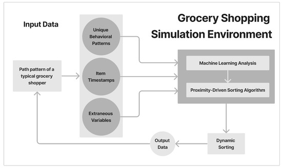
Figure 1.
Conceptual framework. The system design provides the optimal grocery shopping list based on the proximity of items, reducing the dwell time of grocery shoppers.
The proximity-driven sorting algorithm utilizes the patterns and sequences learned from the first step, then sorts the items according to the determined optimal order. Additionally, the dynamic sorting creates an adaptable design with the real-time data considering the factors such as first item selected, i.e., availability, and store dynamics. Lastly, the output data are the optimized and sorted list of grocery items designed to increase the shopper efficiency, thus reducing the amount of time spent in the supermarket.
This study employs a comparative experimental research design to analyze the performance of the grocery shopping navigation that utilizes a sorted shopping list with agglomerative clustering, affinity propagation clustering, and a normal or unsorted shopping list. This allows for determination of the specific elements or mechanisms behind each algorithm that give it an edge over other algorithms, and to determine if it improves the performance of a shopper in terms of their dwell time.
The method consists of one control group and one experimental group. The former is simulated without the supervision of software-based behavioral control mechanisms, while the latter is exposed to sorting algorithms using agglomerative clustering and affinity propagation clustering.
3.2. System Analysis and Design
1. Unity-based simulation
The development of the grocery store simulation was performed in the Unity 2D development platform. The simulation environment, as shown in Figure 2, follows a top-down view of the entire grocery store with approximate measurements of the store layout. We selected a typical supermarket model for the simulation and conducted indoor mapping, detailing layout, aisles, sections, and product placement. To ensure accuracy, the researchers visited the chosen location in person and measured the dimensions. The simulation incorporates five essential elements.
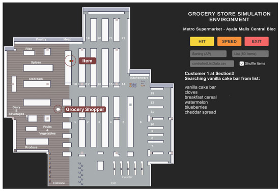
Figure 2.
Grocery store simulation environment with layout based on actual supermarket.
a. Grocery shopper
The grocery shoppers for this experiment are virtual entities created with different movement speeds, decision times, and section entry and exit probabilities; and the A* pathfinding algorithm provided by Unity game engine is used for determining the route for the item to be acquired on the list. Grocery shoppers are presented with a shopping list and navigate through the supermarket, visiting sections based on probability, and scanning items within each section. Since we aim to achieve the fastest possible time to acquire all shopping items, narrowing their behavioral model to an optimal one should increase the effectiveness of the dataset used, as well as eliminating unnecessary data [17]. Figure 3 summarizes the flow for the behavior of the grocery shopper in a simulation environment.
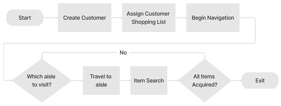
Figure 3.
Behavior of a grocery shopper in a simulated environment. This is the flow for the behavior of a grocery shopper in a simulated grocery environment.
b. Shelf arrangement of items
The positioning of aisles and labels follows the selected supermarket model. The grocery items are objects with assigned names (e.g., fruit, meat, fish, chips, tissue paper, soap, etc.), which are in a similar arrangement to the supermarket model chosen, and these items could also have multiple instances inside the store. These variables have a significant impact on the path that the grocery shopper takes as they roam the grocery store.
c. Shopping list
Grocery shopping lists were prepared with three different sizes, i.e., number of items the list contains. A small list contains 5–7 items, a medium list contains 10–14 items, and a large list contains 15–21 items. The items that are generated on each list are loaded randomly from the 555 items found in the selected grocery store. Moreover, these items do not feature brands or prices. Upon first creation of the grocery shopper, a shopping list is assigned to the shopper. An item is crossed off the list when the grocery shopper locates the item in the section they are currently in until all the items have been purchased.
d. Item acquisition timestamping
In a simulation environment, the assigned shopping list serves as their personal list for the products that they intend to purchase; a collision trigger is used on the simulation which allows the shopper to signal to the system if an item has been acquired (simulating a button-press event upon item acquisition), and automatically lists a timestamp for the item. The first item acquired starts with a timestamp of 0.0 s and immediately triggers a counter that continues indefinitely until the user acquires the last item on the list, which marks the dwell time or the total time it takes the user to finish their grocery shopping. These processes are integral in data validation since dwell time reduction is one of the key desired outcomes of this study.
e. Dynamic list sorting
For the experimental group, the grocery shoppers have the dynamic sorting function on their shopping list. Each time an item is acquired, the list is re-sorted so that items that are in closest proximity are listed at the top. This functionality is only deployed after the machine learning model training completes, since prior to that, there are no data on which to base the sorting. The dynamic nature of the sorting algorithm holds the possibility of memory space constraints or large time complexities; however, the machine learning model has been found to solve the problems mentioned.
2. Software techniques and algorithms
a. Experimentation environment
In order to formulate the sorting algorithm that the experimental shopper group used during the validation phase, the proponents first created an environment which allowed for the integration, modification, and usage of a variety of software techniques and algorithms that ultimately produced the sorting algorithm. This experimental environment was an application built from scratch, removing the restrictions that using third-party software may have posed. The versatility of a custom-built application allowed the proponents to use any technologies that fit their needs and rapidly change any technology that needed to be replaced or modified.
b. Simulation-based crowd-sourcing
During the incremental development of the simulator, the researchers simultaneously gathered initial data using the grocery shopping simulator so that the experimentation phase could be started concurrently. The output data of the simulation were lists whose contents were a pair of item names and timestamps that indicated when the item was acquired relative to the first item acquired. Since we opted for a virtual representation of grocery shoppers, the data were not completely realistic. However, this allowed us to generate a higher amount of data within the given developmental time.
c. Item time difference
Once sufficient timestamps were gathered, the data were first cleaned. The time gap was computed with the time difference between each item’s timestamp and the timestamp of the item that preceded or followed it, using Euclidean distance. The time gap between two items was stored in a dictionary wherein the key was the pair of items and its value was the time gap. Since the total number of items in the modeled grocery store was 555, the combination of items and the size of the dictionary was
f. Proximity matrix tables
The proximity values were normalized and represented through a distance matrix. This provided a clean and easily accessible structure for the data calculated. The table was a NumPy array that dynamically updated the proximity of two items by storing a history of time gaps and updating the normalized values whenever new data were obtained. Matrices were also used as inputs later on in some of the algorithms that were used. These tables also served as a tool for analyzing the data gathered and identifying behavioral patterns that were present, which was used to further calibrate the algorithm.
d. Clustering algorithms
The researchers used three different clustering algorithms. The k-means algorithm was initially used, but it was configured to use a precomputed matrix as the input since the default parameter of the algorithm would calculate its own distance matrix after extracting features from the dataset, and this was not applicable to our dataset which was already represented as a distance matrix.
However, this machine learning model had a flaw; k-means clustering requires a value k to be provided, as shown in Figure 4, wherein k is the number of clusters that needs to be formed, and is the centroid which the data points try to conform to. This algorithm requires constant adjustment of the value k until such a time when the clusters formed are ‘best-fit’. This was not suitable for our objective since we wanted the algorithm to estimate the optimal number of clusters. Although there are workarounds to make the model autonomously choose a value for k, this is very counter-intuitive as the algorithm itself works best under supervision.
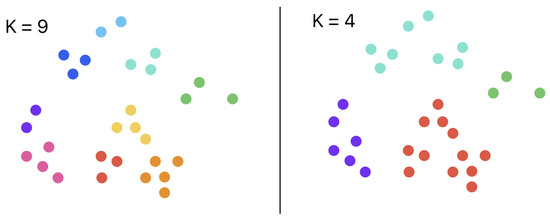
Figure 4.
Illustration of example K-means clustering model with k clusters.
The second approach used a type of unsupervised hierarchical model called agglomerative clustering, which was also tuned to receive a precomputed matrix. This method is a bottom-up approach that initially considers all data points to be their own cluster. The clusters that are closest together are merged recursively until a certain number of clusters or a distance threshold is met, after which the final clusters are formed, as illustrated in Figure 5. There are different linkage criteria that can be used to determine the distance between sets of observations; average linkage was selected, a middle ground between the tendency of small linkage to produce loose clusters and the tendency of complete linkage to produce tight clusters. However, agglomerative clustering is not fully unsupervised, in the sense that the model requires the number of clusters to be specified like in k-means clustering, or alternatively, a distance threshold can be specified to avoid explicitly setting the number of clusters. The second option was more applicable for this study since we wanted to make sure items that were physically close together were clustered, thus the distance threshold was set to a value that corresponded to the decision-making time and the traveling time set in the simulator.
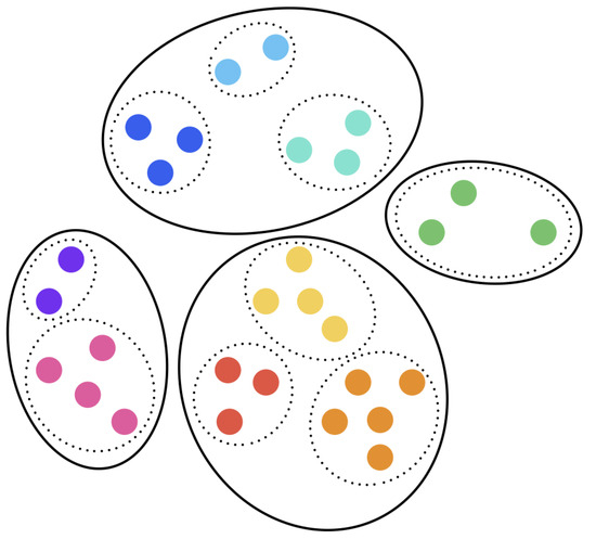
Figure 5.
Illustration of Agglomerative clustering model.
Although this approach nearly fulfilled all our requirements, there was still a major issue that the model did not fully address. The two aforementioned clustering algorithms work well with high-density graphs, but not so well with sparse ones. Both algorithms would require a connection between all 307,740 pairs to function properly, and it would take the simulator a very long time to accomplish that task.
An imperfect but effective way to solve this is by setting distances for items with no connection to a very large number such as 10,000, thereby telling the model that those two items are dissimilar. Of course, this means that the algorithm cannot accurately discern the proximity of two items if data are insufficient, i.e., it will not cluster items that are supposed to be close together but do not have a connection stored yet. Thus, the DProSA algorithm is expected to have higher efficiency for larger datasets.
A third algorithm was used to solve the issue of requiring denser graphs to work well. Affinity propagation is a clustering technique that is best fit for sparse graphs. As depicted in Figure 6, it works by calculating the “responsibility” and “availability” of each data point, and a high value for both makes that data point an exemplar. Responsibility measures the similarity of that data point to other data points, while availability measures how much support it receives from other data points. This machine learning model calculates the two criteria through multiple message exchanges that eventually converge to a set of exemplars which are “representatives” of clusters. Other data points then conform to the exemplars which best represent them. Exemplars are often located in dense regions of the data, but the model does not require a strongly connected graph. The model achieves this by using a similarity matrix instead of a distance matrix or dissimilarity matrix. The input matrices were converted accordingly for this algorithm.
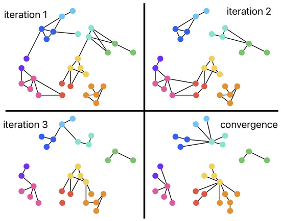
Figure 6.
Illustration of Affinity propagation clustering model with four iterations.
The machine learning models were used to cluster the items so they were grouped according to closest proximity. These clusters are essentially ‘sections’ of the supermarket where item acquisition activity for those sets of items is higher than in other areas, and the timestamps represent the items. In order to reduce the time complexity of the sorting process and save memory space, clustering helped us by treating the clusters as one group of items. During the sorting process, the distance between each item no longer had to be referenced, as in the brute force method; instead, only the clusters were sorted.
e. Dynamic sorting
As mentioned earlier, this approach to sorting the shopping list is expected to be much faster than brute force since the sorting occurs for groups of items rather than individual items. Dijkstra’s algorithm is used to traverse all clusters for a given shopping list in the shortest amount of time. Handlers are also included in cases wherein an item is foreign, i.e., it was newly added. An item within the cluster is selected as the first point, and this is marked as a visited node. From the current visited node, after determining the nearest unvisited node, it is now be selected as the new current visited node. This process is repeated until the last unvisited node is selected. The important element in the sorting algorithm is the sorting key, which is composed of the following:
- −1 if the item is in the anchor cluster (first cluster in the shortest path); 1 otherwise.
- The cluster number of the item or float (‘inf’ if not found).
- The index of the cluster in the shortest path or float (‘inf’ if not found).
- The index of the item in the original list.
These elements determine how the shopping list is sorted. In order to determine the shortest path between all clusters, the algorithm references the proximity matrix and calculates the distance between clusters. As a shopping guide, this optimized list expects that the order of the items will not necessarily be followed in actual scenarios; thus, the sorting algorithm can dynamically re-sort whenever an item is acquired. The acquired item becomes an “anchor” which becomes the starting point of the path traversal algorithm, and the route is dynamically adjusted based on the anchor.
3.3. Integration of Machine Learning in Simulation
Figure 7 illustrates the adopted system architecture for this study, integrating the ML-DProSa with the Unity simulation environment. Python serves as the platform for executing ML-DProSA tasks, while Unity is utilized for simulation purposes. Since these environments do not natively interoperate, we establish communication between them using a socket-based server connection. In this setup, the server initiated in Python awaits a client connection, representing the simulation environment.
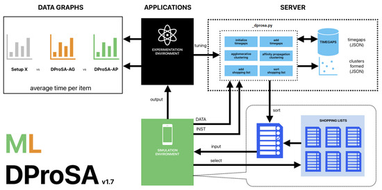
Figure 7.
Adopted system architecture for the integration of the simulation environment to the ML-DProSA.
Upon initiating the simulation, it tries to establish a connection with the server’s address. Once the connection is successfully established, the client transmits data strings, which are subsequently decoded by the server.
There are specific instructions sent by the client that could be handled by the server. Upon successful decoding, the server invokes ML-DProSA to execute the specified instruction.
The specific instructions that the server can decode are as follows:
- Perform cluster: The server invokes ML-DProSA to perform specific clustering method to the contents of a specific directory. This directory information is also embedded in the data string transmitted by the simulation.
- Perform sort: The server calls ML-DProSA to execute a sorting operation based on the string received from the simulation, subsequently returning the sorted string.
- Perform normal: This instruction prompts the server to perform a pseudo-sorting operation, where it refrains from executing any sorting and simply returns the original string received from the simulation.
3.4. Validation and Deployment
3.4.1. Dwell Time Comparison
The validation for this study was conducted in the simulation environment. The grocery shoppers performed various shopping trips with provided sets of randomly generated shopping lists in three setups. The first setup did not use any sorting algorithm; the second setup used the agglomerative clustering variant of ML-DProSA; and the third setup used the affinity propagation clustering variant of ML-DProSA. The following configurable settings were used:
- Limited item pool to choose from;
- Small, medium, or large number of items per list;
- Number of shoppers per test.
Different combinations of these settings allowed us to determine the performance of either variant of ML-DProSA in different scenarios. The average dwell times of shoppers, both with and without sorting algorithms, were recorded, and then, represented in various graphs. The simulation speed was also scaled up to ×20 of the normal speed, resulting in faster data gathering while still retaining the actual time that the character took to travel from one item to the other. The decision-making time was also set to 10 s, which is the average time taken for the verbal responses of people that were asked in the grocery store during our indoor store mapping for the layout. These augmentations to the simulation were accounted for in the post-processing of the simulation output data.
3.4.2. Continuous Learning
During the simulation of the algorithm deployment, the model continues learning from the data stream, aiding in the validation of the inputs and ensuring that the data are still relevant. The simulator clusters the items after certain intervals of shoppers, which shows the effect of clustering in relation to shopping efficiency. Store layout changes cannot be avoided, thus the machine learning model identifies changes in the proximity calculations and makes the appropriate changes in the proximity matrix. Scenarios such as when items are moved, replaced, or removed altogether are accounted for by resetting the proximity values for affected pairs after a certain number of runs.
4. Results and Discussions
The overall goal of this study is to determine if the machine learning-assisted dynamic sorting algorithm devised in the previous section successfully accomplishes the proposed hypothesis. The validation process is discussed in the sections that follow, providing insights into the effectiveness and reliability of the implemented algorithm.
4.1. Data Collection and Analysis
4.1.1. Precomputing Clusters
Before the actual validation runs, two training sets were generated by running 1000 shoppers with unique lists containing 15–21 items; the first set used a pool of 60 out of 555 items and the second set used all 555 items. These were used to precompute clusters for the DProSA setups during the validation runs.
4.1.2. Simulation Output
The output data of the simulation is a file in comma-separated value format, wherein the first column is the item name; the second column is the timestamp; and the third column is a flag that checks if the pick-up is valid or not. The two important parts that need to be extracted from this output file are the total number of items and the last timestamp recorded for a particular shopper. This timestamp is also known as the “dwell time” of the shopper. The dwell time over the total number of items gives us the performance metric for this validation study: the average time per item.
4.1.3. Test Setups and Configurations
Multiple simulations were simultaneously executed across different computers, each configured according to specific setups detailed in Table 2. The first setup, labeled X, ran the base simulator with no sorting algorithm to assist the virtual grocery shoppers. The second setup, labeled DProSA-AG, ran the base simulator with dynamic sorting assistance that used the agglomerative clustering approach to form the proximity clusters. The third setup, labeled DProSA-AP, ran the base simulator with dynamic sorting assistance that used affinity propagation clustering to form the clusters. All setups had the same shopping list contents per iteration, but the contents were shuffled randomly.

Table 2.
Summary of the simulation setup.
The simulator was built with three configurable settings: total number of items to choose from; range of the shopping list size; and the number of shoppers to run. Given these settings, the simulators were executed across five distinct configurations, each representing a unique scenario, as summarized in Table 3:
- Scenario 1a determines the algorithms’ learning rates when there are fewer items per shopper.
- Scenario 1b determines the algorithms’ average learning capacity.
- Scenario 1c determines the algorithms’ learning rates when there are more items per shopper.
- Scenario 2 determines the performance of the algorithms in an uncontrolled scenario wherein shopping lists and contents vary per shopper.
- Scenario 5 utilizes the full 555 item pool to show the performance of the algorithms in more diverse item pools.

Table 3.
Summary of the test configurations.
Table 3.
Summary of the test configurations.
| Config | Item Pool | List Size | Unique Lists | Runs |
|---|---|---|---|---|
| 1a | 60 items | 5–7 | 100 | 4 |
| 1b | 60 items | 8–14 | 100 | 4 |
| 1c | 60 items | 15–21 | 100 | 4 |
| 2 | 60 items | 5–21 | 100 | 1 |
| 3 | 555 items | 5–21 | 100 | 1 |
4.1.4. Post-Processing and Cleaning of Data
It was also declared that the simulation speed was to be scaled up to ×20 of the normal speed to avoid lengthy simulation times. To account for this, the researchers scaled the timestamps to the appropriate time using the equation:
where
- is the new dwell time;
- is the current dwell time;
- L is the length of the list;
- R is the scale factor in seconds.
The equation works by removing the decision-making time set in the simulation, which was set to 10 for each item in the list. A scale factor, denoted by R, was added for each item in the list to account for the actual speed of the simulation. This scale factor was a random value generated from 110 s to 130 s, resulting in the new dwell time averaging at a 2 min increase from the previous dwell time.
4.2. Key Findings
4.2.1. Performance of the Three Setups
Initially, the three setups were executed without employing the proposed machine learning-based assistive algorithms to validate whether significant differences in terms of average shopping time among them were present. This baseline assessment aimed to ensure that all three setups were unbiased before proceeding with validation runs. As depicted by the solid lines shown in Figure 8, over the course of 100 shoppers, the average time per item for every block of shoppers was consistent across all three setups, with variation within half a second. For clarity, the trend lines (dash lines) for of the three setups reveal a smooth pattern, interpreted as a consistent performance throughout the entire duration of 100 shopping scenarios, thereby underscoring the reliability of the baseline assessment.
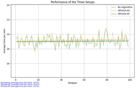
Figure 8.
Performance of the setups. The three setups have similar performances when no sorting is applied, indicating no bias in any of the three.
The same data were scaled using the scaling Equation (1), and its output is graphed to show if there are significant changes during the scaling process. As shown in Figure 9, the scaled data are almost identical to the data in Figure 8, verifying the legitimacy of the equation used. Furthermore, this result allowed us to continue the validation runs while ensuring the scaled data are valid.
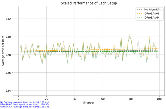
Figure 9.
Scaled performance of the setups. Applying the scaling equation defined previously yields similar performances, showing that the scaling process is unbiased.
4.2.2. Improvement for Each Setup
The first configuration, Figure 10, shows the earliest signs of improvement compared to the others. It can be said that the algorithm performs well when shopping lists are smaller. In particular, the agglomerative clustering variant performs better than its affinity propagation counterpart, averaging 1–2 s faster when it comes to the average time per item. It can be deduced that DProSA-AG performs better than DProSA-AP because fewer linkages are required for smaller lists. It was also observed that there were times that DProSA-AP performed better than DProSA-AG; in such instances, the shopping lists’ items had not yet obtained a sufficiently robust linkage. As the same shopping lists were run again, the agglomerative model had already obtained proximity data from previous runs.
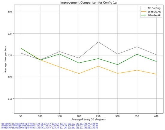
Figure 10.
Configuration 1a. This scenario depicts the performance of the three setups for small-sized lists. The average time gap for every 50 shoppers is also shown.
The medium-sized list, as shown in Figure 11, has the least definitive result of the three list configurations. Aside from the drop in average time per item for the fourth group of 50 shoppers, the performances of the algorithms do not seem to portray any relevant improvement. The reason for this could be the range of the item count for the medium-sized lists, which was set to 8–14. This wider spread results in a mix of smaller and larger lists, which results in the overall performance being normalized.
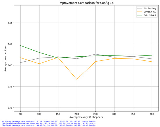
Figure 11.
Configuration 1b. This scenario depicts the performance of the three setups for medium-sized lists. The average time gap for every 50 shoppers is also shown.
The previous statement is further substantiated in the performance data of large lists. As shown in Figure 12, agglomerative clustering loses its advantage over affinity propagation due to larger lists not being able to form robust linkages when the number of lists is smaller. Even though there are more items in each individual list, the pairwise connections formed are not substantially greater since there are only 100 lists. The ratio between shopping list item count and pairwise connections formed is much more efficient for smaller lists than larger lists. In fact, for the shopping list used in configuration 1c, only 1303 pairs were formed; in contrast, the shopping list used in configuration 1a generated 838 pairs. As such, it is expected that DProSA-AP would be able to perform much better since it does not require robust linkages as much as DProSA-AG.
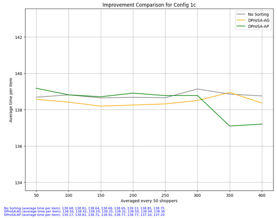
Figure 12.
Configuration 1c. This scenario depicts the performance of the three setups for large-sized lists. The average time gap for every 50 shoppers is also shown.
After analyzing the algorithmic trends and patterns for varied list sizes, 100 shoppers with a mixed assortment of small, medium, and large lists were looped five times. The first scenario used a pool of 60 items, and the clusters were precomputed before run-time via the 60 item pool training set. The first 200 shoppers do not exhibit any significant changes; however, by the third group of 100 shoppers, the average dwell time for these shoppers dropped by 13 s and 20 s for DProSA-AG and DProSA-AP, respectively. This number is already significant considering the number of shoppers that it took to achieve this; by the end of the fifth loop, the average dwell time for the last 100 shoppers reached 28 s for DProSA-AG and DProSA-AP.
In configuration 2, as shown in Figure 13, since there are only 60 items, the linkage between pairs achieves robustness sooner. This is the reason why the agglomerative clustering variant performs similarly to the affinity propagation variant. Configuration 3, as shown in Figure 14, challenges DProSA-AG as it introduces a full 555 pool of items to generate lists from. Immediately after the precomputation of clusters, DProSA-AP performs better than DProSA-AG, maintaining this advantage throughout the five loops. By the end of the fifth loop, although DProSA-AG sees some improvements compared to the no-DProSA setup with a 10 s difference in dwell time between the two, the affinity propagation variant is able to achieve a 40 s improvement to the average dwell time of grocery shoppers. The affinity propagation model’s ability to work with sparse matrices elevates its performance even when there are multiple pairwise connections not yet formed.
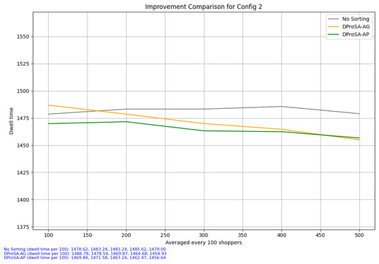
Figure 13.
Configuration 2. This scenario shows the improvement in terms of dwell time for 100 shoppers looped 5 times. The shopping lists for the shoppers were generated from a pool of 60 items.
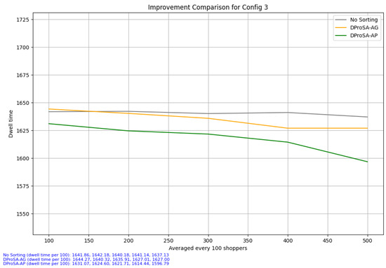
Figure 14.
Configuration 3. This scenario shows the improvement in terms of dwell time for 100 shoppers looped 5 times. The shopping lists for the shoppers were generated from a pool of 555 items.
In summary, the ML-DProSA variants, specifically agglomerative and affinity propagation clustering, have demonstrated a significant reduction in average dwell time and improved optimization of shopping paths compared to scenarios without product sorting implementation, as evidenced by the simulation results. These outcomes underscore the potential effectiveness of the proposed method for real-time applications. The dynamic nature of these methods adapts well to diverse store layouts and shopper behavior, consistently enhancing navigation efficiency across varied scenarios. However, to further validate these promising results, future research should include validation against real-world data and ground truth observations.
4.2.3. Cluster and Sorting Time Analysis
In the analysis of the clustering and sorting time of the algorithm, Table 4 is used as a guide in determining the specific number of items in each label.

Table 4.
Number of items based on the label.
From the graph shown in Figure 15, DProSA-AG shows a better clustering time than DProSA-AP. DProSA-AP takes an average of 20% more time than DProSA-AG. However, during the sorting time of each algorithm shown in Figure 16, DProSA-AP shows better sorting time than DProSA-AG, with an average of 45% less time than DProSA-AG. Although both algorithms have differences in the clustering and sorting time, it should be noted that these values are almost negligible when it comes to their actual usage.
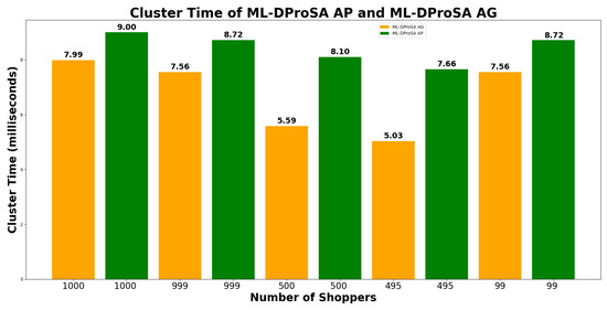
Figure 15.
Clustering times of DProSA-AG and DProSA-AP. The graph is based on the 60 item pool data.
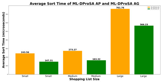
Figure 16.
Average sorting times of DProSA-AG and DProSA-AP. Each bar is differentiated based on the size of the list and the algorithm used.
4.3. Limitations of the Study
Although the simulated grocery environment proved valuable in the experimental phase of this study, the inherent limitations of replicating the real-world shopping experience pose a challenge in fully validating ML-DProSA’s assistive capabilities. Despite the simulator’s ability to capture various aspects of shopper behavior, it falls short of accurately representing the unpredictable and multifaceted nature of actual grocery trips. This shortcoming prevents the validation phase from comprehensively evaluating the algorithm’s ability to handle the nuances and complexities of real-world grocery shopping scenarios.
Two limitations of this study remain to be addressed. First, instances of the same item appearing in multiple, widely separated locations can distort the accuracy of cluster formation. Second, while a basic mechanism was implemented to handle changes in item placement, removal, and other instances of item movement, the implemented fix resets important data for that item, requiring the model to relearn the data to properly assign the item to a new cluster.
Furthermore, this study did not incorporate multiple grocery store layouts into the simulation. This limited scope was intentional, as the researchers initially focused on demonstrating the algorithm’s potential effectiveness. While the study successfully demonstrated that the algorithm reduces shopper dwell time, there was a possibility of a negative outcome. Including multiple grocery store layouts without first validating ML-DProSA’s performance would have unnecessarily complicated the study. However, now that there is conclusive evidence of ML-DProSA’s positive impact on the grocery shopping experience, future studies could explore the aforementioned aspects of the grocery shopping experience.
4.4. Recommendations and Future Directions
The findings of this study open up intriguing possibilities and introduce a new set of questions that warrant exploration in subsequent research. One avenue for further investigation involves enhancing the core functionality of ML-DProSA by integrating additional machine learning models. Specifically, incorporating word embedding models could contribute to delineating relationships between items within the context of grocery store product arrangements. This extension aims to refine cluster relationships among items, facilitating the inclusion of unclustered or poorly clustered items into groups that exhibit significant semantic similarities.
Furthermore, recommender system models present another avenue for exploration. These models could play a pivotal role in predictive recommendation by discerning the consumer type of a grocery shopper based on their shopping list’s content. Subsequently, the model could cross-reference this information with a dataset of preferences, ultimately enhancing the algorithm’s sorting capabilities and improving the traversal path for more accurate recommendations. This multifaceted approach of leveraging word embedding models for cluster refinement and recommender system models for predictive recommendation on top of the currently established clustering and sorting algorithms holds promise for advancing the capabilities and effectiveness of ML-DProSA in the realm of grocery shopping optimization.
However, the applicability of this algorithm extends beyond grocery stores. ML-DProSA’s optimization capabilities can have a substantial impact in other settings with multiple items or objects arranged in rows of shelves and storage units. An immediate application that comes to mind is the optimization of warehouse management. If ML-DProSA is further developed to such a point where it is highly accurate and reliable, it has the potential to simplify the logistical challenges associated with tracking and managing large warehouses. This could empower personnel to navigate warehouse layouts more effectively.
5. Conclusions
In conclusion, when considering grocery shopping optimization, affinity propagation emerges as the more suitable clustering algorithm due to its compatibility with distance-based clustering and its effectiveness in handling sparse matrices. Affinity propagation excels in scenarios where pairwise connections among items are limited, making it well suited for optimizing grocery shopping lists with potentially sparse relationships between products. On the other hand, while agglomerative clustering can be adapted for grocery shopping optimization by appropriately setting distance thresholds, it is more reliant on dense graphs to perform optimally. This makes agglomerative clustering a viable option when numerous pairwise connections exist, but it may not be as efficient in scenarios with fewer linkages between items. In the context of grocery shopping, where the complexity of product relationships can vary, the adaptability and efficiency of affinity propagation position it as the preferred choice for effective and nuanced optimization strategies.
Furthermore, it is essential to consider the impact of varying shopping list sizes on the performance of affinity propagation and agglomerative clustering. Affinity propagation tends to shine when dealing with larger shopping lists due to its ability to handle sparse matrices effectively, making it a robust choice for comprehensive grocery shopping optimization. Conversely, agglomerative clustering exhibits better performance with smaller lists by setting appropriate distance thresholds, capitalizing on the strength of dense graphs. An intriguing approach would involve a dynamic strategy that leverages both algorithms based on the size of the shopping list. However, it is crucial to note that the presented conclusions are drawn from a dataset with 500 data points. To ascertain the algorithms’ robustness and performance across a broader spectrum of shopping scenarios, conducting larger validation runs could yield more comprehensive and reliable results, enhancing the overall understanding of their effectiveness in grocery shopping optimization. This would enhance the adaptability of the machine learning-assisted proximity-driven sorting algorithm in response to the constantly evolving retail environment.
Author Contributions
Conceptualization, P.V.A., G.C. and L.G.C.J.; methodology, P.V.A., G.C. and L.G.C.J.; development and validation, V.A., J.I. and J.M.P.; investigation, V.A., J.I. and J.M.P.; data curation, V.A., J.I. and J.M.P.; writing—original draft preparation, V.A., J.I. and J.M.P.; writing—review and editing, P.V.A., G.C. and L.G.C.J.; visualization, P.V.A. and G.C.; supervision, P.V.A. and G.C.; project administration, P.V.A.; All authors have read and agreed to the published version of the manuscript.
Funding
This research received no external funding.
Data Availability Statement
The original contributions presented in the study are included in the article, further inquiries can be directed to the corresponding author.
Conflicts of Interest
The authors declare no conflicts of interest.
References
- Wagner, J. The Grocery Report 2019: Nielsen; Nielsen: New York, NY, USA, 2019. [Google Scholar]
- Gumasing, M.J.J.; Prasetyo, Y.T.; Persada, S.F.; Ong, A.K.S.; Young, M.N.; Nadlifatin, R.; Redi, A.A.N.P. Using Online Grocery Applications during the COVID-19 Pandemic: Their Relationship with Open Innovation. J. Open Innov. Technol. Mark. Complex. 2022, 8, 93. [Google Scholar] [CrossRef]
- Leone, L.A.; Fleischhacker, S.; Anderson-Steeves, B.; Harper, K.; Winkler, M.; Racine, E.; Baquero, B.; Gittelsohn, J. Healthy Food Retail during the COVID-19 Pandemic: Challenges and Future Directions. Int. J. Environ. Res. Public Health 2020, 17, 7397. [Google Scholar] [CrossRef] [PubMed]
- Goić, M.; Levenier, C.; Montoya, R. Drivers of customer satisfaction in the grocery retail industry: A longitudinal analysis across store formats. J. Retail. Consum. Serv. 2021, 60, 102505. [Google Scholar] [CrossRef]
- Nair, S.R. Analyzing the relationship between store attributes, satisfaction, patronage-intention and lifestyle in food and grocery store choice behavior. Int. J. Retail. Distrib. Manag. 2018, 46, 70–89. [Google Scholar] [CrossRef]
- Paulin, M.; Neumann, N.; Schreieck, M.; Wiesche, M. Examining navigation and orientation problems in retail stores. Int. J. Inf. Manag. 2018, 47, 119–129. [Google Scholar]
- Bourlakis, M.; Mamalis, S.; Sangster, J. Planned versus unplanned grocery shopping behaviour: An empirical study. In Proceedings of the Fifth WSEAS International Conference, Citeseer, Athens, Greece, 15–17 September 2005; pp. 1–6. [Google Scholar]
- Sabanoglu, T. Total Retail Sales Worldwide from 2020 to 2025. Statista 2022. Available online: https://www.statista.com/statistics/443522/global-retail-sales/ (accessed on 8 June 2024).
- Wästlund, E.; Reinikka, H.; Norlander, T.; Archer, T. Attractive displays improve shoppers’ mood and satisfaction. J. Retail. Consum. Serv. 2015, 22, 175–180. [Google Scholar]
- Jayananda, P.; Seneviratne, D.; Abeygunawardhana, P.; Dodampege, L.; Lakshani, A. Augmented reality based smart supermarket system with indoor navigation using beacon technology (easy shopping android mobile app). In Proceedings of the 2018 IEEE International Conference on Information and Automation for Sustainability (ICIAfS), Colombo, Sri Lanka, 21–22 December 2018; IEEE: Piscataway, NJ, USA, 2018; pp. 1–6. [Google Scholar]
- Hu, G.; Feldhaus, P.; Feng, Y.; Wang, S.; Zheng, J.; Duan, H.; Gu, J. Accuracy improvement of indoor real-time location tracking algorithm for smart supermarket based on ultra-wideband. Int. J. Pattern Recognit. Artif. Intell. 2019, 33, 2058004. [Google Scholar] [CrossRef]
- Kulyukin, V.; Gharpure, C.; Nicholson, J. Robocart: Toward robot-assisted navigation of grocery stores by the visually impaired. In Proceedings of the 2005 IEEE/RSJ International Conference on Intelligent Robots and Systems, Edmonton, AB, Canada, 2–6 August 2005; IEEE: Piscataway, NJ, USA, 2005; pp. 2845–2850. [Google Scholar]
- Yan, J.; Zlatanova, S.; Lee, J.B.; Liu, Q. Indoor traveling salesman problem (itsp) path planning. ISPRS Int. J. Geo-Inf. 2021, 10, 616. [Google Scholar] [CrossRef]
- Behera, M.P.; Mishra, V. Impact of store location and layout on consumer purchase behavior in organized retail. Anvesha 2017, 10, 10–21. [Google Scholar]
- Clark, L. Going for growth. Chem. Drug 2003, 15, 42. [Google Scholar]
- Cil, I. Consumption universes based supermarket layout through association rule mining and multidimensional scaling. Expert Syst. Appl. 2012, 39, 8611–8625. [Google Scholar] [CrossRef]
- Page, B.; Trinh, G.; Bogomolova, S. Comparing two supermarket layouts: The effect of a middle aisle on basket size, spend, trip duration and endcap use. J. Retail. Consum. Serv. 2019, 47, 49–56. [Google Scholar] [CrossRef]
- Titus, P.A.; Everett, P.B. The consumer retail search process: A conceptual model and research agenda. J. Acad. Mark. Sci. 1995, 23, 106–119. [Google Scholar] [CrossRef]
- Breugelmans, E.; Campo, K.; Gijsbrechts, E. Opportunities for active stock-out management in online stores: The impact of the stock-out policy on online stock-out reactions. J. Retail. 2006, 82, 215–228. [Google Scholar] [CrossRef]
- Seeja, K. Solving travelling salesman problem with sparse graphs. In Proceedings of the AIP Conference Proceedings, Bodrum, Turkey, 4–8 September 2019; AIP Publishing LLC: Long Island, NY, USA, 2019; Volume 2186, p. 170011. [Google Scholar]
- Dijkstra, E.W. A Note on Two Problems in Connexion with Graphs. Numer. Math. 1959, 1, 269–271. [Google Scholar] [CrossRef]
- Hmeljak, D. Design and Evaluation of a Virtual Environment Infrastructure to Support Experiments in Social Behavior; ERIC: Budapest, Hungary, 2010. [Google Scholar]
- Hart, P.E.; Nilsson, N.J.; Raphael, B. A Formal Basis for the Heuristic Determination of Minimum Cost Paths. IEEE Trans. Syst. Sci. Cybern. 1968, 4, 100–107. [Google Scholar] [CrossRef]
- Ada, A.H.D.; Cortez, I.P.Q.; Juvida, X.A.S.; Linsangan, N.B.; Magwili, G.V. Dynamic Route Optimization using A* Algorithm with Heuristic Technique for a Grocery Store. In Proceedings of the 2019 IEEE 11th International Conference on Humanoid, Nanotechnology, Information Technology, Communication and Control, Environment, and Management (HNICEM), Laoag, Philippines, 29 November–1 December 2019; pp. 1–6. [Google Scholar] [CrossRef]
- dela Cruz, J.C.; Magwili, G.V.; Mundo, J.P.E.; Gregorio, G.P.B.; Lamoca, M.L.L.; Villaseñor, J.A. Items-mapping and route optimization in a grocery store using Dijkstra’s, Bellman-Ford and Floyd-Warshall Algorithms. In Proceedings of the 2016 IEEE Region 10 Conference (TENCON), Singapore, 22–25 November 2016; pp. 243–246. [Google Scholar]
- Hui, S.K.; Fader, P.S.; Bradlow, E.T. Research note—The traveling salesman goes shopping: The systematic deviations of grocery paths from TSP optimality. Mark. Sci. 2009, 28, 566–572. [Google Scholar] [CrossRef]
- Larson, J.S.; Bradlow, E.T.; Fader, P.S. An exploratory look at supermarket shopping paths. Int. J. Res. Mark. 2005, 22, 395–414. [Google Scholar] [CrossRef]
- Gao, L.; Su, J.; Zhao, L. Understanding the Relationship Between Grocery Shopping Motivation and Shopping Behavior: A Mixed-Methods Approach. J. Food Prod. Mark. 2018, 24, 23–40. [Google Scholar]
- Kaufman, L.; Rousseeuw, P.J. Finding Groups in Data: An Introduction to Cluster Analysis; Wiley Series in Probability and Statistics; John Wiley & Sons: Hoboken, NJ, USA, 1990; Volume 1. [Google Scholar] [CrossRef]
- Vadivel, P.S.; Karthika, B.; Robinson, Y.H.; Krishnan, R.S.; Rachel, L.; Sundararajan, S. An Intelligent IoT-Driven Smart Shopping Cart with Reinforcement Learning for Optimized Store Navigation. In Proceedings of the 2023 International Conference on Emerging Research in Computational Science (ICERCS), Coimbatore, India, 7–9 December 2023; IEEE: Piscataway, NJ, USA, 2023; pp. 1–6. [Google Scholar]
- Xu, X.; Chen, X.; Ji, J.; Chen, F.; Sanjay, A.V. RETaIL: A machine learning-based item-level localization system in retail environment. In Proceedings of the Collaborative Computing: Networking, Applications and Worksharing: 13th International Conference, CollaborateCom 2017, Edinburgh, UK, 11–13 December 2017; Proceedings 13. Springer: Berlin/Heidelberg, Germany, 2018; pp. 221–231. [Google Scholar]
- Paolanti, M.; Liciotti, D.; Pietrini, R.; Mancini, A.; Frontoni, E. Modelling and forecasting customer navigation in intelligent retail environments. J. Intell. Robot. Syst. 2018, 91, 165–180. [Google Scholar] [CrossRef]
Disclaimer/Publisher’s Note: The statements, opinions and data contained in all publications are solely those of the individual author(s) and contributor(s) and not of MDPI and/or the editor(s). MDPI and/or the editor(s) disclaim responsibility for any injury to people or property resulting from any ideas, methods, instructions or products referred to in the content. |
© 2024 by the authors. Licensee MDPI, Basel, Switzerland. This article is an open access article distributed under the terms and conditions of the Creative Commons Attribution (CC BY) license (https://creativecommons.org/licenses/by/4.0/).