Abstract
Automated greenhouse production systems frequently employ non-destructive techniques, such as computer vision-based methods, to accurately measure plant physiological properties and monitor crop growth. By utilizing an automated image acquisition and analysis system, it becomes possible to swiftly assess the growth and health of plants throughout their entire lifecycle. This valuable information can be utilized by growers, farmers, and crop researchers who are interested in self-cultivation procedures. At the same time, such a system can alleviate the burden of daily plant photography for human photographers and crop researchers, while facilitating automated plant image acquisition for crop status monitoring. Given these considerations, the aim of this study was to develop an experimental, low-cost, 1-DOF linear robotic camera system specifically designed for automated plant photography. As an initial evaluation of the proposed system, which targets future research endeavors of simplifying the process of plant growth monitoring in a small greenhouse, the experimental setup and precise plant identification and localization are demonstrated in this work through an application on lettuce plants, imaged mostly under laboratory conditions.
1. Introduction
Nowadays, the use of dedicated, sensor-based growth status monitoring systems in cultivating greenhouse crops, while enhancing precision in controlling the crop environment, is regarded as a crucial and distinctive method in precision agriculture. This approach enables the efficient and accurate management of crop production, while also meeting the requirements for producing high-quality and safe agricultural products. Moreover, a meticulously controlled greenhouse environment effectively minimizes the unnecessary consumption of resources such as CO2, water, and fertilizer, thereby enhancing the industry’s environmental sustainability [1]. The incorporation of an intelligent monitoring system enhances energy-saving and emission reduction outcomes while possessing the ability to forecast extreme greenhouse conditions [2]. Among other intelligent greenhouse monitoring techniques, various sensor imagers and integrated imaging modalities are employed in high-throughput phenotyping platforms to gather data for the quantitative analysis of intricate characteristics associated with plant growth, productivity, and resilience to biotic or abiotic stressors such as diseases, insects, drought, and salinity. These imaging methodologies encompass machine vision, multispectral and hyperspectral remote sensing, thermal infrared imaging, fluorescence imaging, 3D imaging, and tomographic imaging (e.g., X-ray computed tomography) [3]. Moreover, the use of artificial intelligence, big data, deep learning, the Internet of Things (IoT), and other cutting-edge technologies in greenhouse monitoring procedures are regarded as beneficial advancements that nowadays enhance unmanned greenhouse management, significantly facilitate plant growth monitoring, and control procedures [2,4].
Data analysis and evaluation tasks are becoming more and more common in precision agricultural research, while data acquisition tasks are supported by expanding computer vision techniques and access to data from various sensors [5]. A combination of data acquisition, data modeling, analysis, and evaluation is also carried out in the constantly evolving field of image classification and object detection based on Convolutional Neural Networks (CNNs) and Deep Convolutional Neural Networks (DCNNs). For example, a DCNN-based intelligence method for estimating above-ground biomass in the early growth stage for winter wheat is proposed in [6]. Another method that utilized digital images and the application of a CNN for growth-related monitoring traits, like the fresh and dry weights of greenhouse lettuce, was proposed in [7]. Moreover, some indicative yet successful application examples of the many developed and further optimized image processing algorithms and computer vision techniques that utilized CNN and DNN methods include the development of plant disease recognition models, based on leaf image classification [8,9], the simultaneous extraction of features and classification for plant recognition [10], simulated learning for yield estimation and fruit counting [11], automated crop detection in seedling trays [12], crop yield prediction before planting [13], weed detection [14], pest detection [15], automatic sorting of defective lettuce seedlings grown in indoor environments [16,17], tip-burn stress detection and localization in plant factories [18], and many others [19,20,21,22,23]. Deep learning techniques have shown significant advancements in machine and computer vision tasks concerning feature learning, thus facilitating plant data analysis and plant image processing while demonstrating great potential in the agricultural industry. The automatic features’ extraction from raw plant image datasets, for purposes such as prediction, recognition, and classification, involves the progressive formation of higher level image features to be composed from low-level features through the hierarchy [24]. These paradigms and the previously reported application examples outline a promising and non-destructive approach for treating massive amounts of data in various applications related to plants, including detection and localization, growth analysis, crop prediction, and plant phenotyping. The progress made in these areas highlights the potential of deep learning in advancing our understanding and management of plant-related processes.
However, deep learning-based algorithms, although often showing superior performance traits related to accuracy (e.g., compared with traditional approaches to computer vision-based tasks, like plant identification), require careful fine-tuning to achieve the highest desired outcomes. At the same time, a very large amount of generic data and available datasets is needed for pre-training and achieving the desired performance of the models [24]. Moreover, their success relies significantly on the availability of an appreciable amount of computing resources that can be utilized to successfully accomplish the assigned tasks. Furthermore, it is quite common for some approaches to utilize plant images during model training that exhibit either optimal imaging acquisition properties or disregard real field conditions. For example, these images might showcase a white or monochrome backdrop encircling the plant, the absence of soil surrounding the plant, or a meticulously prepared monochrome substrate devoid of any fertilizers near the plant. Additionally, these images may lack the presence of moss or depict plants that are not potted, among various other factors. Nevertheless, traditional machine vision, computer vision, and machine learning methods that rely on basic image processing techniques and fundamental machine learning algorithms (e.g., K-means, SVM, KNN, linear regression, random forest, etc.), especially when targeting smaller image datasets with fewer sensors utilized, still continue to be valuable, preferable, and valid for all the aforementioned factors [25,26,27,28,29,30].
Growers and researchers can reap several benefits by integrating machine vision, computer vision, and robotics for plant growth monitoring in greenhouses but also in the field [22,30,31,32]. For example, a constructed machine vision-guided lettuce sensing and features’ monitoring system (color, morphological, textual, and spectral) is illustrated in [33]. In [34], an urban robotic farming platform is demonstrated on a laboratory scale for lettuce recognition and subsequent water irrigation tasks. An integrated IoT-based, three-device-system of autonomous moving platforms, aiming to facilitate precision farming and smart irrigation by utilizing the data collected from many sensors, was introduced in [35]. A robotic platform with a vision system and a custom end effector, targeting the harvesting of iceberg lettuce under field conditions, is presented in [36]. In [4], a methodology is presented that combines the application of a digital camera and artificial intelligence for growth prediction as well as the harvest day and growth quality of lettuces in a hydroponic system. An automated growth measurement system for Boston lettuce in a plant factory is developed in [25]. Each lettuce was iteratively photographed, with the cameras moving in predefined increments along the planting beds. Plant growth curves were presented by the authors after applying image processing techniques for each plant’s contour detection and the subsequent estimation of each plant’s area and height. Similarly, agricultural tasks, like a flower harvesting mechanization, implemented as a three-axis design with mechanical parts based on a computer numerical control machine (CNC) and utilizing YOLOv5 deep learning techniques for the localization and detection of flowers, is presented in [37]. In [14], a small-scale Cartesian robot, aiming at performing functions like seed sowing, spraying, and watering in predefined locations, is presented. The system utilizes YOLO for weed detection. In a similar fashion, in [38], a small farming CNC machine for irrigation, planting, and fertilizer application in predefined locations is implemented. Moreover, the utilization of hyperspectral imaging sensors, along with the potential adaptation of other low-cost, yet promising multispectral compact designs [39,40] suitable for integration into robotic platforms, can be effectively utilized in agricultural applications to perform repetitive activities such as the plant photography that the present work focus on, but also facilitate other interesting agricultural procedures and applications such as fruit harvesting or even fruit ripening assessments.
However, a common challenge within the field of computer vision, particularly in the wider scope of agriculture, pertains to the accessibility of datasets for researchers to utilize in order to conduct tests and experiments while developing algorithms or devices. Creating custom image datasets is frequently required, a process that can be quite time consuming, lasting for hours or even days. Additionally, monitoring greenhouse plants and collecting data, especially for research purposes using basic hand-held cameras, can be a laborious, time-consuming, and monotonous undertaking. Moreover, to achieve the necessary accuracy and repeatability during plant image acquisition, the possibility of possessing a robotic mechanism that acts as a reliable and robust recoupment of a human photographer/crop researcher seems to be valuable. With the help of robotic cameras, plant images can be acquired at any time of the day, at the “exact same spot”, under almost identical conditions (e.g., same viewpoint, distance, and same shooting angle) without the need for a human’s presence in the field. The images can then be sent to a remote computer, and the researcher can further systematically monitor plants’ health and growth-related traits, with minimal effort.
With these factors in mind, the objective of this study was to develop an experimental, low-cost, 1-DOF linear robotic camera system tailored for automated plant photography. As an initial evaluation of the proposed system that targets, as an ongoing project, simplifying the process of plant growth monitoring in a small greenhouse in our university’s facilities, this study presents, in detail, the hardware materials used to construct the robotic experimental setup, the software developed for its operation, as well as the methodology followed to assess its construction and movement accuracy along with its ability to accurately identify and localize plants, demonstrated through the examination of lettuce plants primarily in laboratory settings. In this context, the present work focuses on top-view images of the plants, and most image processing and real-time lettuce detection operations are related to the task of color segmentation and the successful analysis of their total projected leaf area and contour, since the top-view images contain more information to monitor plant health than the side-view images [29,41].
Apart from this introductory section, the rest of the manuscript is organized as follows: Section 2 presents the proposed 1-DOF linear robotic camera system’s hardware design and construction in detail along with its software pipeline. Additionally, the experimental setup devised to assess the system’s movement accuracy and repeatability is thoroughly explained. Moreover, Section 3 demonstrates the results and the respective discussion over the conducted experiments related to the main aspects of the robotic camera system, and more specifically, its movement’s accuracy and repeatability assessment and plant identification and localization ability, while also discussing its limitations; it also provides related work from other research studies and a future research outlook. Finally, Section 4 concludes the manuscript.
2. Materials and Methods
2.1. System’s Design and Construction
A low-cost, 1-DOF linear robotic camera system, named RoboPlantDect, targeting the systematic image acquisition of plants and facilitating future research endeavors like greenhouse growth plant monitoring procedures, was fully designed and constructed from scratch (Figure 1a–h). The initial idea originated from the need for an automated plant photography system for lettuce cultivation research purposes in our university’s facilities, without having to sacrifice many human resources for field observations. The original purpose was to monitor, from above, lettuce seedlings, at the stage of four true leaves, growing in plastic pots and arranged in a single row inside an unheated saddle roof double-span greenhouse covered with polyethylene film. However, except from the thorough inspection and consideration of the usual design factors like the cost and the availability of the construction materials, the ease of assembly, and the maintenance costs, a few more prerequisites were defined early in the design process phase. More specifically, among others, these included the following:
- The system should be able to automatically detect and accurately localize the spaced plants that are growing apart in plastic pots, positioned in a fully randomized design, in a 3 m long row;
- The system as a whole, should be lightweight and portable but also easily scalable if needed in order to facilitate its easy positioning for monitoring other rows inside the greenhouse too;
- To ensure that the linear robotic camera system can precisely reach each of the target plants, the actuator must exhibit sufficient precision in its movement. Upon reaching the target, the system should capture a high-resolution, color, top-view image with the plant ideally centered;
- With none or minor modifications and/or software adjustment settings, the linear robotic camera system could also be applicable for other plant species’ monitoring research and investigation purposes in hydroponic systems (e.g., spinach, sweet peppers, herbs, and strawberries, to name a few);
- The system should not, in any manner, obstruct the plants’ growth;
- Detected and localized plant images along with all the plant growth-related data measurements performed, together with the datalogging information, should be automatically stored locally, but also transmitted to a remote location and synched in a secure and transparent manner;
- No human intervention should be necessary at any stage of plant detection and monitoring.
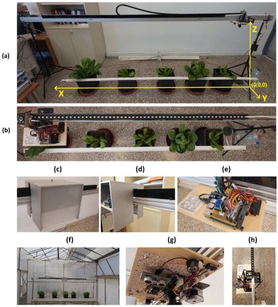
Figure 1.
View and details of the constructed RoboplantDect 1-DOF linear robotic camera system. (a) Global system of coordinates, applied to the robotic camera system. Transformations and measurements involving the various coordinate systems of interest are performed in reference to this coordinate system, which belongs to the “right side” of the device. The camera is moving in the X-axis only. The left side is considered to be the other beam’s end, where the left tripod is secured; (b) panoramic top view of the system, moving towards the far left; (c,d) side views of the water-resistant plywood box cover, with sliding plexiglass window in front; (e) top view of the carriage; (f) system setup in the greenhouse, with lettuce arranged in a single row; (g) detailed view of the carriage’s bottom side, showing the camera, LEDs, distance sensors, and limit switches mounted; (h) top view, showing the system in “home” position, on the far right side.
The implementation of the computer vision-guided system is divided into two parts, and more specifically, into the following: (a) the system’s design and construction, which describe and present the hardware parts and the implementation details that comprise the whole system assembly and (b) the system’s software programming andworkflow, which describes the system’s software building blocks and the complete pipeline. The detailed, full list of materials and parts that were designed, constructed, assembled, or purchased, is presented in Table A1 of Appendix A. In Figure 2, a simplified schematic diagram shows the complete system’s pipeline.
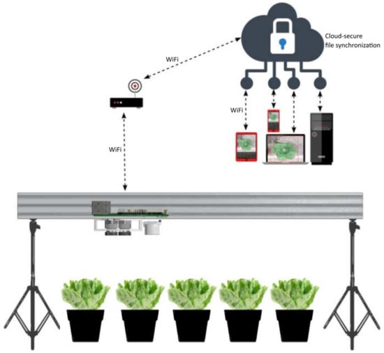
Figure 2.
Simplified schematic showing the proposed computer vision-based system’s pipeline.
2.1.1. Hardware: Stable and Moving Parts
The RoboPlantDect system was designed to monitor lettuce plants growing in a greenhouse inside plastic pots and further arranged in 3 m long rows. A prerequisite design definition was that the whole construction should be lightweight and that it could be placed above any row of plants inside the greenhouse, by a person or two, without disassembling the whole device each time. Following this requirement, the main structure of the system was assembled mainly by combining high quality, lightweight linear aluminum extrusions.
For this purpose, three V-Slot 2060 () aluminum beams [42] (Figure 3c) were connected in series, one 1.5 m and two 1 m long, since the desired 3.5 m long single beam could not be found at the time of device’s construction at the local market. By placing the 60 mm side vertically, no bending was observed along the whole run of the 3.5 m long rail. V-Slot’s aluminum profile construction characteristics feature the internal V-shaped channels and V-grooves that further permit the linear V-Slot wheels’ smooth movement (Figure 3c,d). For firmly connecting the V-slot 2060 in series, tee nuts were placed in the top and bottom ends of the V-Slot connections at both sides (Figure 3d).
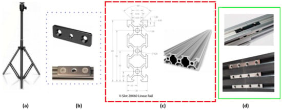
Figure 3.
Main hardware frames and support parts. (a) Camera tripods used for system’s support; (b) tripod mounting plates that were mounted at both ends of the 3.5 m long rail structure; (c) type of V-slot aluminum profiles used; (d) double tee nuts (up) and quad tee nuts (down) used for the three V-Slot 2060 aluminum profiles’ connection.
Moreover, at both edges of the 3.5 m long beam, two camera tripods (Figure 3a) [43] capable of extending up to 210 cm height were attached to support the whole structure. These tripods are very lightweight, and they significantly facilitate height adjustments. They also have the added benefit of being able to be positioned in any uneven area, which is a typical sight in greenhouses. Finally, at the top of each tripod, a mounting plate ¼ was placed (Figure 3b) to ensure that both tripods were fitted to the aluminum beams securely.
A cable drag chain organizer (Figure 4a) was placed on top of the beams to ensure the proper grip and smooth movement of the power cable. Made from nylon, with a bend radius of 18 mm and external dimensions of , it proved to be an ideal choice for cable management. To ensure that the cable organizer always stayed on top of the V-slot beams and did not fall on either side (during system movement), two pieces of a aluminum beam were cut, drilled, and further used as both protective sidewalls and as a guide (Figure 4b). The latter aluminum supports were secured with spring-loaded ball nuts (Figure 4c). This prevents unwanted movement of the nut in the slot and allows the nuts to be inserted in a vertical position, as they will not slip due to gravity. As a carriage for the main construction platform, a V-slot Gantry Plate set of (Figure 4d) [44] was used and under it, a piece of marine plywood (dimensions ) was secured. Finally, another small piece of plywood beam (dimensions ) was fixed to the carriage to link the carriage with the drag chain and the cables. The system’s power switch was attached to this beam. To protect the carriage (and all the electronic components mounted on it) from the accidental use of the greenhouse’s mist irrigation system, a water-resistant plywood box was designed, constructed, and used as the system’s protection cover (Figure 1c,d). The final construction turned out to be robust, adaptable, and dependable.

Figure 4.
In (a), the cable drag chain used for cable management is shown; in (b), side views show the custom-made aluminum beams that were used as the cable drag chain’s guide/sidewall protection; (c) spring-loaded ball tee nuts used for aluminum beam fixation; (d) the carriage platform.
The reference system of coordinates is considered attached firmly to the right tripod, and its origin () is shown in Figure 1a. Every linear movement of the 1-DOF camera system (i.e., translation along the X-axis) is performed in relation to this reference system. The linear movement is converted in the software into the corresponding motor’s steps, so as to precisely instruct the stepper motor to move the carriage platform, and subsequently, the whole cameras’ system structure, to achieve the desired pose.
2.1.2. Hardware: Motor, Controller, and Transmission
The movement of the carriage was performed using one high-torque, bipolar stepper motor (12 V DC, 0.4 A/phase, 200 steps/revolution, size NEMA17) with a 1.8° full step angle [45]. The stepper motor was positioned beneath the carriage and oriented with the shaft pointing upwards in order to link it with the timing belt and create a linear rotor drive system (Figure 5a).
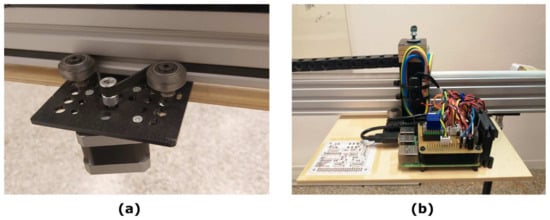
Figure 5.
In (a), a view of the stepper motor, GT2 Timing Pulley-12T and GT2-type timing belt along with the V-Slot wheels and the carriage platform (V-slot Gantry Plate). The platform is secured to a piece of marine plywood in (b), and the TMC2209 stepper motor driver with its dedicated heatsink is shown mounted on a custom PCB Raspberry Pi shield (described in Section 2.1.3).
A GT2 aluminum timing belt pulley with 12 teeth was attached to the shaft of the stepper motor (Figure 5a). Its small diameter retained the torque produced by the stepper motor. In addition, a 3.5 m long GT2-type timing belt (2 mm pitch, 6 mm width, made of neoprene and fiberglass materials) was attached to the two ends of the beam, which was used to transmit motion. As the axis of the stepper motor rotated, the timing pulley forced the carriage to move across the beam. The control of the stepper motor was achieved with a TMC2209 V2.0 [46] stepper motor driver connected to the Raspberry Pi and used a microstepping factor of 2 (e.g., half step), resulting in 400 steps per revolution of the motor shaft (Figure 5b). The calculated steps per mm for the linear motion produced by the belt was found to be . Here, is the number of steps per revolution of the motor, is the microstepping factor, is the pitch, and is the number of teeth on the pulley attached to the motor shaft.
2.1.3. Hardware: Sensors, Auxiliary Electronics, and Raspberry Pi
Two SPDT momentary microswitches (model KW4-Z5F150, YueQing Daier Electron Co., Ltd., Yueqing City, Zhejiang, China [47]) with roller levers were used as limit switches (Figure 6a). They were attached at the far left and right of the carriage, so that the carriage could detect the origin and the end points of the line, respectively. When the carriage reached the end of the route, the corresponding microswitch contacted the tripod. In this way, the system determines the start (“home” position) and end positions of the route on the beam. An Arducam synchronized stereo USB camera [48] was used to capture the images (Figure 6e) in the current design. This module consists of two fixed focus cameras integrating OV2710 OmniVision (Santa Clara, CA 95054, USA) CMOS sensors [49] with the same resolution of 2 MP and sensitivity to both visible light (RGB) and infrared light (IR). In this work, the RGB camera was mainly used for the plant recognition task. The eight LEDs installed on the module board are infrared LEDs and are automatically turned on when the IR camera is used.
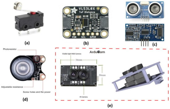
Figure 6.
View of the sensors and the main auxiliary electronics: (a) terminal limit switch; (b) distance ToF sensor; (c) ultrasonic distance sensor; (d) infrared LED board; and (e) stereo USB camera module.
This stereo USB camera was chosen based on its synchronization capabilities, as well as its similar characteristics and features to both RGB and IR cameras. If images corresponding to the same scene are captured by the two cameras, they can be further combined with a previous image registration processing method to obtain the relevant Normalized Difference Vegetation Index (NDVI) images of the plants, thus obtaining useful data on the health the plant itself. However, the NDVI-related calculations are reserved for future work. To ensure the sufficient illumination of the plants during image capture also in the infrared spectrum, two additional infrared LED boards (3 W high power 850 infrared LED, 100° FOV, [50]) were used (Figure 6d). The built-in, adjustable resistor was adjusted to allow the LED to turn on in all ambient lighting conditions. A 1 m long LED strip (60 white LED 3528/m, input voltage 5 V DC) with the USB plug removed was also used complementarily to ensure the sufficient illumination of the plants in the visible spectrum.
In this study, two different low-cost distance sensors were used to provide complementary distance measurements during image capture and as the carriage moved linearly over the plants. The first was a VL53L0X sensor module [51], which contains a 940 nm laser source and a matching sensor that can detect the “time of flight” (ToF) of the light bouncing back to the sensor (Figure 6b). This distance sensor supports two modes of operation: normal mode, where the maximum measurable range is about 1200 mm, and long-range mode, where the maximum measurable range is 2100 mm. The results are noisier in the latter case [51]. Both modes provide the same output data precision, that is, 1 mm. In the present study, this distance sensor was programmed to operate in normal mode and demonstrated its accuracy, particularly for distance measurements within the range of approximately 600 mm (Figure 7a,c), The detection angle was 25 degrees.
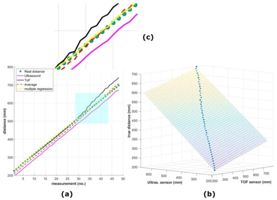
Figure 7.
(a) Scatter plot showing the relation of height (distance) measured in the experiment with the ToF (in black) and ultrasonic (in pink) distance sensors, their average readings (dashed red line), and the best fitted line after applying multiple linear regression (yellow), as related to the true height (small filled green–blue circles); (b) same best fitted line after applying multiple linear regression as in (a) but as a 3D scatter plot; (c) zoomed-in image of the cyan rectangular region (colored figure online).
An additional inexpensive sensor with a slightly wider detection angle of 30 degrees was also employed to obtain distance measurements by combining the readings from both sensors. The HC-SR04 ranging module (Figure 6c) [52] includes an ultrasonic transmitter, a receiver, and a control unit for determining the distance to an object. This sensor measures a range from 2 cm to 400 cm with an accuracy of 0.3 cm. The camera and the sensors were positioned in very close proximity to one another. For the purposes of this work, a specific experiment was performed to test the calibration process of both distance sensors, while examining the possibility of the existence of linear dependence in the datasets with those of manual measurements (true height). In this study, a sample (3D-printed box with dimensions ) was placed sequentially every 1 cm at a distance ranging from approximately 225 mm to 700 mm below the lens of the RGB camera and the sensors (Figure A2a, of Appendix A), and 48 RGB images were captured. The sensors were employed to calculate the distance of the sample from each sensor. The purpose of this experiment in the present work was twofold: The first was to test the calibration process of both distance sensors and to establish a relationship of their outputs as compared to the ground truth height by performing measurements in a range that matches the final application (Figure 1f). The second was to gather insight regarding the scale conversion of pixels to physical measurement units such as millimeters (mm), which are necessary for analyzing measurements like the lettuce diameter or the total projected leaf area. By analyzing the object in all these images (e.g., by simple averaging the distance in pixels of both different sides of the sample object, as appear in the images versus the distance in reality in millimeters), the scale () as well as the factor () along the various distances/depths could be estimated (Figure A2b, of Appendix A). From these calculations, the resolution can be approximated. Furthermore, accurate distance calculations for a lettuce plant as depicted in an image (such as its maximum diameter) can be achieved with reasonable precision, assuming that the two extremity control points on the leaves that are utilized for the maximum diameter calculation and belong to its contour’s perimeter lie nearly in the same focal plane, such that they appear approximately at a similar distance from the camera. However, all measurements related to the lettuce diameter and its area in this study are presented in pixels. Although this approach does not provide absolute measurements in metric units, it continues to be valuable, since it enables the relative comparative analysis of lettuce plants, since they are monitored using the same imaging system.
Nevertheless, prior to fitting a specific model to the acquired data using the 2 sensors, we initially investigated if a linear relationship could be established. For this purpose, correlation coefficient matrices were formed, considering a pairwise variable combination of the average readings of 30 measurements per height distance acquired with each sensor (all results converted to mm) and the manual measurements as well. Since the three correlation coefficient matrices that were formed (Table 1) were too close to 1, there was a strong indication that the measurements acquired with the different sensors in pairs could be linear correlated.

Table 1.
Correlation coefficient matrices between sensors and manual measurements.
In Figure 7a,c, the scatter plot shows the relation between the respective measurements of height using each distance sensor, their simple average, and the best fitted line after applying multiple linear regression with an interaction term (also depicted in Figure 7b), as compared to the true height measured manually. The data measured with both sensors were treated as predictors and the true height as the response. The regression coefficients for the linear model that was utilized in this study are shown in Equation (1) below.
The maximum of the absolute value of the data for this model (maximum error) was calculated to be , which is a sufficiently small value and much smaller than any of the sensors’ data values used, indicating that this model accurately follows the measured data of both sensors. Moreover, the fit to the data had the same value for both the correlation coefficient and the adjusted correlation coefficient , with and root mean square error Thus, we conclude that according to the experimental height measurements and the analysis performed, the linear model as described in Equation (1) above fulfills the distance measurement requirements for the purposes of the current work.
To control the fan (mentioned below), the LEDs, the infrared LEDs, and the relay that controls the stepper motor driver, 2N2222A NPN transistors were used, which can handle the current required for these devices and the necessary resistors. An ordinary 12 V DC 2 A power supply was used to power the stepper motor and cooling fan. Finally, to connect all the necessary devices and electronic components, a simplified electronic circuit (Figure 8a) and a printed circuit board (PCB) (Figure 8b) were designed using EasyEDA software ver. 6.5.20 (Figure 8a). JST male/female connectors (JST XH 2.5 mm) were used to connect all devices to the circuit board. The control of the relay and the stepper motor driver, the control of the distance sensors, the limit switches, and the infrared LEDs, as well as the image acquisition, processing, and storage were carried out by a computing unit small enough to fit on the cart and powerful enough to handle all the tasks required. The Raspberry Pi 4 - Model B - 8 GB [53] proved to be ideal because, among other things, it supports WiFi, integrates USB ports, and has sufficient computing power and 8 GB of RAM to process the captured images.
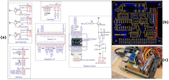
Figure 8.
In (a), the simplified electronics schematic of the part’s interconnections with the Raspberry Pi is shown, and in (b), the designed custom PCB Raspberry Pi shield is shown. The PCB was designed to be one-sided. The two red lines correspond to short-wire bridges between the top and bottom copper layers. Two wires were soldered for that purpose during our custom fabrication of the circuit. In (c), a top view shows the Raspberry Pi fitted in the carriage together with the designed Raspberry Pi shield that houses all the electronic parts.
The official Raspberry Pi USB-C power supply (output voltage: 5.1 V DC, max. power: 15.3 W) was used to power the Raspberry Pi and all peripheral sensor devices. Given the high temperatures that can be achieved in a greenhouse, heat sinks coupled with a 12 V fan (the latter to also move the dust away) were used to cool the Raspberry Pi (RPI) (Figure 8c).
2.2. System’s Software Programming and Workflow
2.2.1. NIR and RGB Cameras’ Calibration
The geometric calibration of both cameras was conducted by assuming a pinhole camera model and a frontal parallel arrangement. This calibration process involved the utilization of a known-size asymmetric checkboard pattern consisting of 22 × 15 squares, with each side measuring 25 mm. The checkboard pattern was supported by a wooden flat surface, which was securely mounted on a robotic platform (Figure A1b, Appendix A). The entire setup was positioned at a distance from the cameras’ lenses that approximately matched the expected maximum height of the potted lettuces in the final application, ranging approximately 35 to 70 cm. Next, a total of 15 pairs of images were taken, with each pair consisting of a left and right image. These images were captured from different 3D positions and orientations, ensuring that the inclination of the checkerboard did not exceed 35 degrees relative to the plane of the cameras during each image pair capture. The images were saved in an uncompressed format, such as a PNG. The resulting dataset consisted of 30 images, which were then processed using the stereo camera calibration tool in MatlabTM, Computer Vision ToolboxTM. This processing allowed for the calculation of various parameters related to each camera’s intrinsic parameters, distortion coefficients, and extrinsic camera parameters. These parameters included the radial and tangential distortion, intrinsic matrix, focal length, principal point, and mean reprojection error. The NIR camera’s translation and rotation matrices, as well as the fundamental and essential matrices, were computed in relation to the RGB camera. These computed values were then compared to the manufacturer’s datasheet (Arducam, OV2710 Dual-lens module) [54] whenever possible. Table A2 of Appendix A presents some of the noteworthy parameters that were calculated. Accurately determining the pose (position and orientation) of the NIR camera with respect to the RGB camera is crucial for performing NDVI calculations, especially considering that both fixed cameras have almost identical technical specifications. The proper alignment of the RGB and NIR images is essential to ensure the integrity of the data obtained, even though NDVI calculations are not the focus of this study. Ultimately, the resulting overall mean reprojection error of 0.17 pixels was deemed acceptable for the current scenario.
2.2.2. Software: System Pipeline
The user interface of RoboPlantDect is designed to be intuitive and lightweight. It utilizes the cvui2.7.0 UI library [55], which is built on OpenCV drawing primitives. Through this interface, users can easily perform various tasks, as shown in Figure 9a. One of its key features is the ability to set the scheduled time interval for plant recognition and image acquisition, along with specifying the number of plants to be identified. The system is designed to perform several tasks repeatedly.
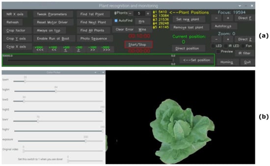
Figure 9.
In (a), the plant recognition and monitoring user interface is shown. In (b), the user’s selection menu for setting the upper and lower thresholds of HSV color values (left side) is shown. Apart from the plant in focus, all other information is filtered out (right side).
Firstly, it identifies the plants and records their precise locations. It then captures images of these plants using both RGB and NIR cameras while also recording the distance of each plant from the cameras based on readings from both distance sensors. Next, the system processes the captured images to determine the total projected leaf contours, diameter, center, total projected leaf area, and centroid of each plant. This information is then combined with the date and time of the recording. All these calculated data values, along with the date and time, are logged into a logfile for future reference. Additionally, the system offers the option to overlay this information onto each image. Furthermore, the acquired RGB and NIR images are saved separately in designated folders.
To ensure data accessibility and backup, the system synchronizes the folders containing the images and recorded data with other dedicated computers through cloud storage. This allows for easy sharing and collaboration among multiple devices.
2.2.3. Plant Finding
A series of procedures must be conducted to identify the plants (see also the flowchart in Figure 10):
- The initial step in the process is crucial as it involves determining the starting position of the carriage. To achieve this, the carriage is moved automatically to the far-right edge of the beam until the right end switch is activated. This position is then labeled as “position zero” (home position).
- Subsequently, the user must have indicated the number of plants for identification. A plant counter is then established and employed to ascertain the number of procedural iterations that will be carried out. In instances where the number of plants remains constant (as is typically the case in practical scenarios, where a specific number of plants exist in a row), this step is omitted, and the number of plants remains unchanged.
- The RGB camera that is utilized for plant recognition is then initialized. An image of is captured for further processing.
- Since the RGB camera has a wide field of view (95° diagonal), it is necessary to crop the image to ensure that only one plant (and potentially small segments of other plants) is present. This operation results in a square frame (cropped image) that features the same center as the original image. This not only helps in better focusing on a single plant, but also reduces the image processing time for the smaller image; the amount of cropping in pixels (a border with the same number for left and right sides as well as the up and down sides) can be determined by the user through dedicated buttons in the GUI (left side in Figure 9a). If denotes the amount of pixels for cropping the image on the left and right sides (width dimension), and similarly, if denotes the amount of pixels for the top and bottom sides (height dimension), the following relationship holds: For example, to result in cropped images, and pixels, respectively. (In this study, the experiments were conducted using cropped images of dimensions and ).
- To filter out any high-frequency noise that may exist, a Gaussian blur (with 11 × 11 kernel size) is applied to the image.
- The image is converted to HSV color space.
- The automatic identification of the plant primarily relies on analyzing its color. To achieve this, users are required to predefine specific thresholds for the Hue (H), Saturation (S), and Value (V). These thresholds determine the range of colors that will be considered as the plant’s color. In this process, the undesired colors are masked out, resulting in a black color in the empty space of the image. To facilitate this procedure, a dedicated menu called “Color Picker” has been incorporated into the graphical user interface (GUI). By pressing the “Tweak Parameters” button, the user can access the “Color Picker” window, where they can adjust the sliders to carefully select the appropriate upper and lower thresholds for the Hue, Saturation, and Value. This ensures that only the colors of the plant are retained, while all other colors are filtered out, leaving a black background. Through an empirical analysis, specific lower and upper thresholds were determined for the examination of lettuces. The chosen thresholds, which proved to be effective and remained unchanged for all the experiments in this study, are as follows: , Saturation , and . Another crucial setting is the exposure value, which can range from 0 to 255. The appropriate value should be selected based on the lighting conditions. In the current application, a value of 200 was chosen during the experiments, which remained unchanged too (the installed LEDs used for illumination proved to be sufficient during all experiments). Additionally, a real-time video is displayed below the sliders to provide users with a convenient visual representation (Figure 8b).
- Having available the upper and lower thresholds for the color values in the HSV space from the previous step, the algorithm proceeds by tracking a particular color (i.e., green) in the image by defining a mask using the inRange() method in OpenCV. After this, a series of erosion and dilation operations are performed to enhance the solidity and distinguishability of the plants, which may result in the appearance of small blobs in the images. For the erosion morphological operation that is performed twice, a (8-neighborhood) structuring element is applied. The dilation operation is performed once with a similar structuring element. The objects present in the image are determined using the findContours() function in OpenCV. In case no objects are found, the process is repeated from the beginning, with a slight shift of the carriage to the left (equal to the number of steps set by the user as Jump Steps).
- If multiple contours are detected, the contourArea() function in OpenCV is applied to discard the smaller ones, retaining only the largest contour. If the identified contour is deemed too small to represent a plant, the process is repeated, with a slight shift of the carriage to the left (empirically set to 2000 steps).
- Once a contour that potentially represents a plant is identified, the minEnclosingCircle() function is utilized to obtain the coordinates of the circle’s center and its radius. This information is then used to draw a circle around the plant.
- If the center of the plant does not align with the center of the image, the carriage is shifted either to the left or right, aligning the camera precisely with the plant (by means of bringing the camera exactly on top of the plant). Subsequently, the entire process is repeated from the beginning. Otherwise, the position of the carriage (and consequently, the plant’s position) is recorded in a file, and the plant counter is increased by one.
- If there are no more plants to be searched for, the procedure concludes.
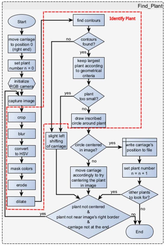
Figure 10.
Flowchart of plant finding procedure.
2.2.4. Image Acquisition, Plant Identification, and Localization
After the plant recognition and the recording of their positions, several measures are implemented to acquire images of the plants and analyze the data collected from the diverse sensors (Figure 11). If the Autofind button has been initially activated, the Find_Plant() function is executed to locate the plants before capturing the final images. The Photo_Sequence procedure will attempt to locate the specified number of plants as indicated on the control panel (number of plants set by the user). In case fewer plants are detected under the moving system, the process of finding plants will be repeated. If, once again, an insufficient number of plants is detected, the finding plants sequence will be repeated for the final time. If the desired number of plants is still not found, the photo sequence will proceed with capturing images of the plants that were detected. Upon completion of the Photo_Sequence, the LED strip will begin to flash, alerting the user to the issue. To resolve the error, the user can press the corresponding button on the control panel (“Clear Error” button, Figure 9a), thereby deactivating the LED strip.
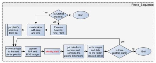
Figure 11.
Flowchart of Photo_Sequence.
Otherwise, a new folder is created with the current date and time as its name. The positions of the plants are retrieved from the relevant file (this function is useful for predefined targets). The carriage is then moved to the next plant’s position. Subsequently, both the NIR and RGB images are taken from the exact same spot after positioning the carriage appropriately. In the RGB image, the plant is identified, and various measurements such as the total projected leaf contour (perimeter), the centroid and total projected leaf area (PLA), etc., are computed and displayed. The carriage is repositioned multiple times in different locations around the identified central point of the plant, with the aim of collecting multiple measurements using the distance sensors. Subsequently, the weighted distance, as described by the linear model in Section 2.1.3 (Equation (1)) between the plant and the sensors, is computed. This information can be utilized further for the plant dimensions (e.g., maximum diameter) calculation. For example, in order to provide a reasonable approximation of the lettuce width (maximum diameter), the simple geometric scenario as shown in Figure A3 of Appendix A can be used. Following this and the triangulation principle, an approximation of a plant’s diameter (D) in metric units (mm) is given as follows: , where in the equation, the letter P denotes the plant’s width as it appears in the RGB imaging sensor in pixels, f stands for the focal length of the camera in mm (i.e., , [48]), and L represents the distance between the camera/sensors and the plant (in mm), as provided by Equation (1). The pixel size is known from [48] to be The procedure, “get data from sensors and compute the plant’s dimensions”, as depicted in the Photo_Sequence flowchart in Figure 11 below, relies on both distance sensors to acquire meaningful measurements at present. This information will be enriched in a future upgrade of the system by fusing data also from the stereo imaging pair. Nevertheless, for the purposes of the present work, dimensions related to growing plants’ parameters are provided in pixels.
Various images including the original, cropped, and images with calculated data overlaid, are saved in the previously created folder. This entire process is repeated until all the available plants have been identified and localized. Currently, the predetermined maximum time that can be devoted for each plant identification is established at a specific value, which has been determined through empirical methods to include a margin of error (. Should the system exceed this threshold, it is deemed a failure and proceeds to identify the subsequent plant. In a usual scenario, the time to detect a plant is by far below the minute.
2.3. Experimental Setup Evaluation and Measurements on Plant Samples
2.3.1. Experimental Setup for System’s Accuracy and Repeatability Evaluation
To assess the precision of the RoboPlantDect’s positioning and its ability to navigate above plants, as well as to evaluate its overall construction, a specific experimental procedure was conducted in the laboratory prior to any other experiments. This experimental setup aimed to evaluate the accuracy and consistency of the robot’s camera positioning along the linear X-axis, as well as assess its construction and mechanical integrity by detecting any misalignments or deviations along the Y-axis, even though the system does not move along this axis. Additionally, adjustments were made to the tripods to ensure that the aluminum beams were parallel to the floor, thus achieving proper positioning along the Z-axis. The evaluation procedure involved repeating the system’s positioning on the same predefined 15 targets for a total of 10 times, allowing for an assessment of the accuracy and repeatability.
The KY-008 laser transmitter module, which emits light at a wavelength of 650 nm and operates at a voltage of 5 V, was installed in a vertical position on the carriage and connected to the Raspberry Pi. A measuring tape was securely fixed on the surface of a CNC cut plywood sheet measuring . This plywood sheet was positioned above 5 empty pots and maintained parallel to the ground at all times, as shown in Figure 12a. The origin of the measuring tape was aligned with the axis origin of the “home” position. In addition to the KY-008 module, a commercial tripod-mounted green laser beam with a wavelength in the range of 510–530 nm was placed near the “home” position. The horizontal cross beam of this laser beam was precisely aligned in parallel with the measuring tape, as depicted in Figure 12a,b.
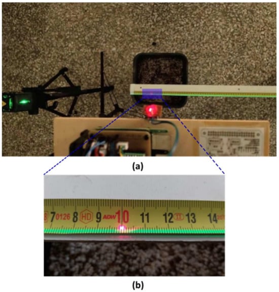
Figure 12.
In (a), the two laser beams used for the evaluation of the system’s accuracy and repeatability are shown. The red laser is mounted vertically on the carriage, while the green laser is generated by the commercial laser tripod and is adjusted to lie down in a parallel axis with the measuring tape. In (b), a detailed close-up view of the measuring tape along with the red laser (spot) and the green laser aligned is shown.
The experiment involved setting 15 targets in incremental steps and recording their positions relative to the “home” position. Throughout the experiment, the red laser beam continuously emitted towards the area of the measuring tape. This setup was repeated for 10 iterations. At the beginning of each iteration, the carriage was set to the “home” position and then moved to each target, simulating a positioning task for the purpose of identifying and photographing plants. The 2D projected red spot of the laser beam on the measuring tape was recorded when the carriage reached each target sequentially. An evaluation of the overall performance of the robotic system was conducted by measuring the distance between the coordinates of the actuator and each target point. Furthermore, the distance between the two vertical laser beams (red and green beams) was manually measured and recorded for each target.
2.3.2. Laboratory Experimental Setup on Lettuce Plants: Image Acquisition and Evaluation Metrics
As an initial evaluation of the system, lettuce seedlings (Lactuca sativa var. Tanius) with four true leaves were transplanted into plastic pots with a capacity of 10 L. These pots were spaced apart in a fully randomized manner in single rows that were approximately 3 m long, with 5 or 6 pots per row. Two experiments were conducted in the laboratory, with both taking place between April and May 2022. In the first experiment, during which the pots containing the plants remained stationary, six baby lettuce seedlings (named A to F) were subsequently detected, localized, and photographed once on the same day and for 15 iterations. The second experiment was conducted in a 4-week interval, in which 5 different lettuce plants (named A to E) were detected, localized, and photographed once every week (growth days 10 to 31 after transplanting). The spacing between the consecutive pots was again fully randomized throughout this specific experiment. In other words, the plants were randomly shuffled and positioned in a row before the experimental detection and photographical procedure each time in this 4-week interval. The plants were watered daily under all circumstances and manually received a nutrient solution in the laboratory. All measurements were carried out between 10:00 am and 14:00 pm. The LEDs of the device used for illumination proved to be sufficient during both experiments.
The degree of detection between the projected leaf area of the lettuce in the ground truth image, which is manually traced to outline the lettuce contour (manual contour delineation), and the corresponding leaf area determined and calculated using the Identify Plant procedure was evaluated using the Intersection Over Union (IoU) metric (Figure 13). This metric provides a ratio that represents the extent of overlap between the projected lettuce area detected in the image and the ground truth area relative to the combined area of both the detection and ground truth. The IoU values range from 0 to 1, where a value of 0 indicates no overlap and a value of 1 indicates a perfect overlap. To calculate the projected leaf area as depicted in the images, all the pixels within the plant area that fall within the identified or manually traced plant contour are considered. The contours are treated as convex polygons. The total projected leaf area for each plant is obtained by summing the product of all the pixels within the plant area and the pixel/mm ratio, if available. The metrics Precision, Recall, and F1 score were also calculated. The Precision metric is derived by dividing the intersection area of each pair by the ground truth area, whereas the Recall metric is computed by considering the intersection area of each pair with the detected area (Figure 13). The F1-score metric is calculated as the weighted average of the Precision and Recall as depicted in Equation (2) below. Additionally, for each defined contour, the centroid was computed. The manual tracing of the lettuces’ contours in the images of the experimental datasets was accomplished using ImageJ ver. 1.53t software (National Institutes of Health, Bethesda, MD, USA).
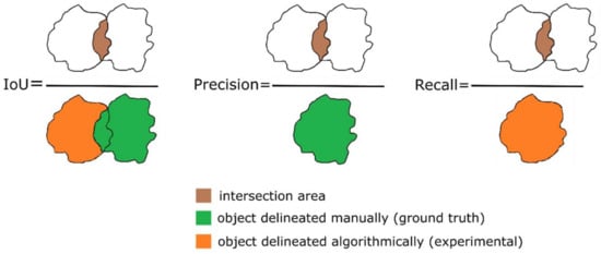
Figure 13.
Simplified schematics of delineation metrics.
In the second experiment, the morphological characteristics of the plants are further examined by considering certain parameters. These parameters are illustrated in the tables and the images provided. Specifically, the Euclidean distance (in pixels) between the centroids and the centers of the minimum enclosing circles is presented for both the experimental and manually traced contours. Moreover, the diameters (in pixels) of these circles are considered, along with the stockiness and compactness (detailed in Section 3.3). Finally, the overall performance and the relative errors are reported.
3. Results and Discussion
The subsequent subsections provide an overview of the performance assessment of the suggested system, encompassing the primary experiments conducted in the laboratory and specifically focusing on the essential metrics. These metrics include the following: (a) the accuracy of the robotic system’s motion, (b) the successful identification and localization of plants, and (c) the determination of various morphological attributes of the plants that are used commonly in plant phenotyping applications for plant growth qualification, such as their diameter, as well as contour-related measurements (i.e., perimeter, area, centroid, etc.). It should be noted, however, that while the operational mechanics of the two low-cost distance sensors utilized in this investigation have been previously elucidated, their installation serves the purpose of collecting additional height measurements pertaining to the scene, rather than solely focusing on the height of the plants and so forth. To analyze measurements like lettuce’s diameter or area using physical measurement units such as millimeters, it is essential to perform the conversion of pixels to that desired unit. Despite the possibility of obtaining a reliable estimation of the pixel/mm scale in our experimental scenarios, as already discussed in Section 2.1.3 and Section 2.2.4, while illustrated also in Figure A2 and Figure A3 of Appendix A, this is reserved for future endeavors, and all measurements of distance and area in this study are presented in pixels. While this approach does not provide absolute measurements in metric units, it enables the comparative analysis of plants, as they are observed using the same imaging system.
Programming for the data analysis, regression, and visualization of the results was performed using MatlabTM, ver. 2018b software (The Mathworks, Inc., Natick, MA, USA). The Raspberry Pi 4 of our robotic camera system was running Raspbian GNU/Linux 10 (buster, kernel: 5.10.63), and its programming was performed using Python, release 3.7.3, and OpenCV 4.5.5.
3.1. Evaluation of the Proposed Robotic System Setup and Its Movement’s Accuracy and Repeatability
Based on the information provided in Section 2.2.3 (also depicted in the flowchart shown in Figure 10), once each plant is successfully identified, a circumcircle is drawn around it to encompass the plant with the smallest possible area (minimum enclosing circle). This circle serves as a boundary for the entire plant, defining the extent of its leaves. Additionally, it is used to align the 2D projected image of the plant, which is obtained by cropping the RGB image. The position of the carriage, measured in steps, is then recorded in a file along with other relevant datalogging parameters. These recorded positions of all the plants detected beneath the aluminum beam act as photographic targets for further analysis.
The objective of this experiment was to assess the potential inaccuracies and misalignments in the construction of the system, as well as its ability to consistently perform the same task (repeatability). Additionally, the experiment aimed to evaluate the error difference between the intended (set) target and the actual outcome (accuracy). In this context, the RoboPlantDect’s system repeatability, refers to the quantitative assessment of its movement at specific points, ensuring consistency across multiple attempts. On the other hand, accuracy pertains to the system’s successful detection and localization of the same target (plant) during each iteration. A Mitutoyo 500-181-30 caliper (Mitutoyo Co., Kawasaki, Japan) with a measurement precision of 0.01 mm was utilized to conduct the manual measurements. Table 2 displays the calculated distances from the center of the target for each iteration of the experiments.

Table 2.
Calculated distance from each of the 15 targets set and for 10 iterations.
Based on Table 2 above, the mean (accuracy) for all iterations for the movement to target No. 6, located at 15,000 steps from the “Home” position, is 1.45 mm, while the standard deviation (repeatability) for the same point is 0.16 mm. Similarly, the mean (accuracy) for all iterations for the movement to target No. 7, located at 19,000 steps from the “Home” position, is 1.65 mm; the standard deviation (repeatability) for the same point is 0.24 mm. The results for these two specific positions but also at 43,000 and 46,000 steps (targets No. 13 and 14), where the mean was calculated to be 1.5 mm and 1.35 mm, respectively (standard deviations of 0 and 0.24 mm correspondingly), are the worst four observations regarding the system’s position accuracy and repeatability for all the experiments conducted. All the other targets were approached with an accuracy estimated in the range 0 to 1.1 mm and with a standard deviation in the range 0 to 0.21 mm. We conclude that the overall system’s positioning accuracy along the X-axis (the axis of linear motion) can be considered in the range 0 to 1.65 mm and its repeatability from 0 to 0.26 mm, respectively. The results presented in Table 2 are also visually depicted in Figure 14a.
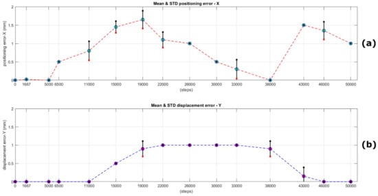
Figure 14.
In the upper graph (a), the mean distance in mm (accuracy) from the ideal positions (targets expressed in steps from “home”) is shown with circles, as well as the standard deviation (repeatability), for 15 iterations, covering the error trends in the whole extent of the possible linear movement along the X-axis. In the lower image (b), the mean displacement error trends (system’s offset along the Y-axis) are shown for the same positions. In both figures, the standard deviation (where is different than zero) is shown visually with small black and red squares (extremity points) and the black line between them. It is evident from the plot that in case of zero standard deviation, both squares coincide with the respective circle’s center in that position (colored figure online).
In Table 3, the measured deviations along the Y-axis through the entire experiment are presented. The recorded outcomes are also visually depicted in Figure 14b. Based on the aforementioned table and the relevant plot, the mean displacement for all iterations when moving towards targets Nos. 7 and 12, as well as the intermediate targets, is approximately 1 mm. This indicates a standard deviation along the Y-axis within this range, which can be attributed to minor misalignments in the junctions of the three V-Slot 2060 aluminum beams that are connected together.

Table 3.
Measured deviation (system’s offset) on the Y-axis, recorded after the experiments that were conducted in various positions covering the full range of linear movement.
Despite securely attaching the beams on both sides with tee nuts, it was not possible to completely eliminate this offset. A potential solution would involve replacing the three aluminum beams, measuring 1.5 m and 1 m in length, with a single piece of aluminum beam measuring a total length of 3.5 m. However, this suggestion is reserved for a future update, as the one-piece beam was not available at the time of implementation. Furthermore, since this observation pertains to a standard offset, it can be compensated for through software means.
Nevertheless, the primary objective of the proposed linear robotic camera system is to monitor plant growth through photography. While it is desirable to achieve a high accuracy in the movement of the carriage, there is no requirement for sub-millimeter precision as would be necessary in medical interventions, for example. We believe that procedures and applications of this nature can be approached with a certain level of tolerance.
3.2. Experimental Results Example on Plant’s Identification and Localization
Figure 15 illustrates, as an example, the process of identifying and localizing six baby lettuce seedlings. The experiment consisted of 15 iterations, during which the pots containing the six plants, positioned at random intervals from each other, remained stationary.
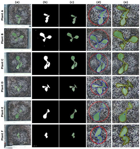
Figure 15.
Plant identification and localization example of the 6 lettuce plants (marked with the letters A through F in the Figure) for the 15 experimental iterations conducted in the laboratory. In column (a), the cropped images of the 6 lettuce seedlings are shown in a single pass (out of the 15 iterations). In columns (b,c), intermediate results of the morphological operations are presented. The final outcomes of each plant contour found (in blue) along with its centroid (small cyan circle), but also the estimated minimum enclosing circle plotted with each center (in red), are depicted in column (d). In column (e), the manually traced plant contours (in yellow squares), along with the respective centroid overlaid in each figure as a small blue circle, are presented for a direct visual comparison (colored figure online).
In each iteration, the system was programmed to initiate the entire process of identification and localization (without any prior knowledge) every 10 min. Each row in Figure 15, labeled with the corresponding plant’s name (plant A to F), displays the basic sequence of plant identification, as depicted in the flowcharts in Figure 10 and Figure 11. Figure 15 column a showcases the six lettuce seedlings photographed in a single pass of the experimental procedure, encompassing all 15 iterations. The columns b and c on the same Figure 15 present the intermediate results of the morphological operations described in the Identify Plant procedure, as outlined in the flowchart of the Plant Finding procedure in Figure 10. Column d of Figure 15 displays the final outcomes of each plant contour found, represented in blue, along with their respective centroid, which is denoted by a small cyan circle. Additionally, the estimated minimum enclosing circle, plotted with each center, is depicted in red. In column e of the same Figure 15, the manually traced plant contours are shown in yellow. Each figure in this column also includes the respective centroid overlaid as a small blue circle, allowing for a direct visual comparison.
Table 4 summarizes the calculated mean and standard deviation of the carriage’s position (in steps) for each of the six lettuce’s (plant A to F) detection and localization task. All locations reported are with reference to the home position. Based on the measurements conducted, it has been determined that in order for the carriage to travel a distance of 3 m along the X-axis, a total of 50,100 steps from the stepper motor are necessary.

Table 4.
Calculated mean and standard deviation for each plant localization (in steps).
Consequently, it can be deduced that the carriage moves at a rate of 1 mm for every 16.7 stepper motor’s steps. According to the information presented in Table 4, the standard deviation (repeatability) for plant A localization in metric units is determined to be 1.43 mm. In the case of locating the target plants B to F, the standard deviations for their localization are as follows: 0.62 mm, 1.94 mm, 0.62 mm, 1 mm, and 1.7 mm, respectively.
Table 5 presents the findings related to the calculated total projected leaf area through experimentation for the 15 iterations involving six baby lettuces, as compared to the area deduced from the manual tracing on the same images.

Table 5.
Evaluation metrics results for the 15 iterations experiment on 6 baby lettuces.
The evaluation metrics IoU, Precision, Recall, and F1 score are utilized to compare these outcomes with the corresponding plant features obtained through manual tracing of the lettuces’ contours.
During the whole run, the RGB and NIR cameras capture images with a resolution of 1920 × 1080 pixels (original images). As mentioned previously the RGB camera is utilized for the plant identification and localization task. Nevertheless, since the calibration parameters are known, a process can be conducted to correct lens distortions in both cameras. Additionally, a rectification process can be applied to the pair of stereo images, enabling the computation of a disparity map for depth estimations and 3D reconstruction or stitching alignment procedures. However, this latter aspect is reserved for future investigations. At present, the identification of plants is performed using the Identify Plant function (Figure 10), which is an ongoing iterative procedure aimed at successfully recognizing different plants. To enhance the efficiency of the image processing process for plant identification, only the RGB images are undistorted prior to being cropped. The color cropped images, which were further analyzed and processed in the specific experiment, had dimensions of 360 × 360 pixels. All images were saved in a PNG format and organized automatically into dedicated folders for each iteration. At the present time, the system logs the original images of both cameras together with all the intermediate (morphologically processed) images until the final, undistorted, cropped colored image outcomes, with the plant centered and circled. Furthermore, the system automatically logged and stored plant growth-related data measurements, along with the datalogging information, both locally and remotely. On average, the entire process, starting from the initial image acquisition at the home position to the identification and localization of the six baby lettuce seedlings, as well as saving all the relevant results, took approximately 6.5 min per iteration. Moreover, the system successfully identified and localized each plant within an average time frame of 55 s.
3.3. Measurements Related to Morphological Characteristics of the Plants
Figure 16 illustrates a detection and localization example of five lettuce plants over a four-week period. The identified plants, labeled as A to E, were consistently photographed every Thursday starting at 12:00 am, throughout the laboratory experiments.
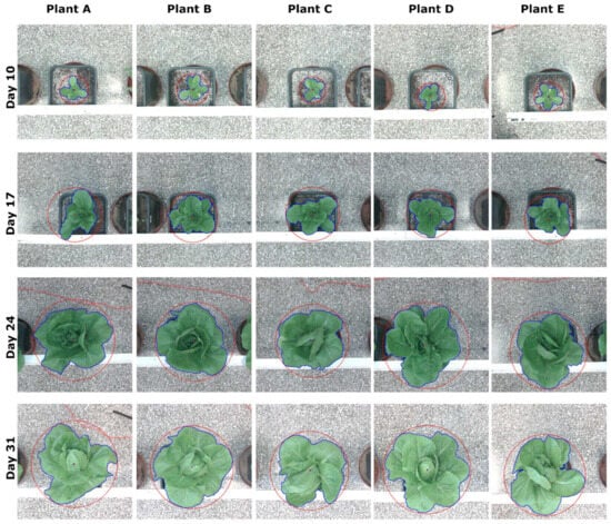
Figure 16.
Plant identification and localization results of 5 lettuce plants, in 4-week growth-stage intervals (color figure online).
The colored cropped images, which were further analyzed and processed in the specific experiment, had dimensions of 888 × 888 pixels. The red circle in the figures represents the minimum enclosing circle of each plant’s contour, which is plotted in blue. Additionally, the small red circle and blue square in each figure indicate the center of the circle and the centroid, respectively. The plot clearly demonstrates the successful detection and localization of all five lettuce plants across different growth stages.
In Figure 17, an enlarged depiction of plant A is provided, illustrating example results of the 4-week growth interval experiment. The experimental outcomes for this plant are presented in the first row of the figure, which aligns with the first column of Figure 16. The second row of Figure 17 displays the corresponding results of manually traced plant contours (represented by yellow squares) for the same images. Additionally, the centroid of each contour is overlaid as a small magenta circle, facilitating a direct visual comparison.
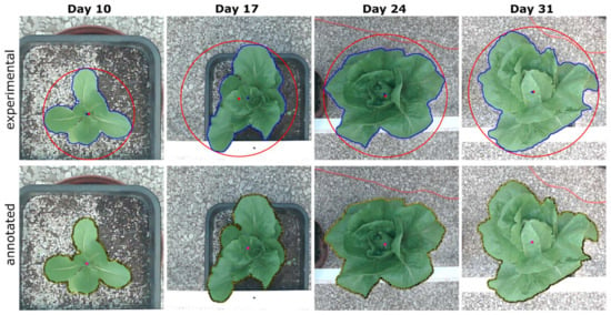
Figure 17.
The first row depicts a zoomed-in version for plant A’s experimental results from Figure 16, for the 4-week growth interval. In the second row, the respective results of the manually traced plant contours (in yellow squares) for the same photographs, along with the respective center of mass overlaid in each one as a small magenta circle, are presented for a direct visual comparison (colored figure online).
Table 6 also displays, as an example, the results concerning the computed total projected leaf area as related to the manual traced outcomes for this 4-week experiment. The evaluation metrics IoU, Precision, Recall, and F1 score are utilized again to compare these outcomes with the corresponding plant features obtained through the manual tracing of the lettuces’ contours.

Table 6.
Evaluation metrics results along with some growth-related parameters for the 4-week experiment.
Table 6 also depicts the Euclidean distance (in pixels) between the centroids of the polygonal shape contour, which is automatically computed experimentally for each plant, as related to the corresponding one calculated from the manual traced plant contours. In a similar fashion, the (in pixels) is reported for the Euclidean distance of the centers of the minimum enclosing circles for each plant.
With the symbols and , the diameters (in pixels) are considered for these circles, which, at the same time, correspond to the maximal distance between two pixels belonging to the lettuce (by means of the longest distance between any two points on its contour’s perimeter outline). Other parameters frequently used for quantifying plant growth using image analysis, which are reported in Table 6 for the specific experiment, are the stockiness and , which is a measure of circularity, or in other words, the roundness, with a value in the range 0 to 1 and compactness and , which expresses the ratio between the area of the plant and the area enclosed by the convex hull (by means of the contour of the smallest convex polygon that surrounds the plant) [30,56,57,58,59,60]. The stockiness involves the area (A) and the perimeter (P) calculations of the leaves and depicts the difference with a circle. It is calculated as follows: In a similar fashion, the compactness is defined as the total leaf area divided by the convex hull area. The subscripts “man” and “exp” are used in the previously referred parameters to indicate the manual calculation and experimentally (automatically) computed values, respectively. Table 7 summarizes the averages (mean and standard deviation of the outcomes) of all metrics and measured parameters depicted in Table 6 for the 4-week experiment. Specifically, for the case of the diameter ( and ), stockiness and ), and compactness ( and ) parameters, the mean and the standard deviation of the absolute difference between the manual and the experimentally calculated values are reported with the symbols D, S, and C, respectively.

Table 7.
Average results (mean and standard deviation) of the evaluation metrics and the growth-related parameters listed in Table 6.
In Figure 18, as an illustrated example, some of the lettuce plants’ parameters that were measured over time (in days) for the 4-week experiments are presented. The measurements were conducted manually and automatically for all five plants labeled A to E, with the data collected once per week. The parameters of the lettuce plants shown in the figure include the total projected leaf area (Figure 18a,b), the maximum diameter (Figure 18c,d), the compactness (Figure 18e,f), and the stockiness (Figure 18g,h) for both manual and automatic calculations in each instance.
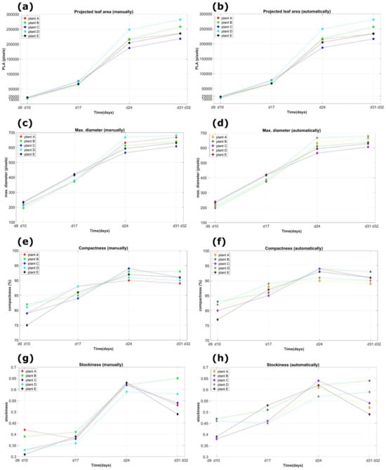
Figure 18.
An example of the measured plant dimensions (both manually and automated) as a function of time (in days) for the 4-week experiments and for all the five plants denoted with the letters A to E. The measurements were performed once every week. The lettuce parameters depicted in the figure concern the total projected leaf area (a,b), the maximum diameter (c,d) the compactness (e,f), and the stockiness (g,h) for the manual and the automatic calculations, respectively, for each case, (colored figure online).
In Figure 19, the detailed visual representation of the detected and ground truth total projected leaf areas overlaid, for all the plants in the 4-week experiment, is presented. The areas’ plots were created as solid polygonal regions defined by 2D vertices. These vertices correspond to each lettuce’s total projected leaf area contour, either manually traced or found experimentally.
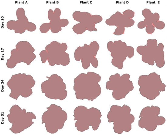
Figure 19.
Visual representation of the detected and ground truth areas overlaid for plants A to E in the 4-week experiment.
In the first 2 rows (Days 10 and 17), the detected (experimental) area is clearly visible with a different color (lighter shade of pink), so as to emphasize the difference in the detection of the plant by our algorithmic procedure. In the last two weeks (Days 24 and 31), the corresponding overlaid, experimentally delineated area of the plant is almost identical to the ground truth and cannot be visually differentiated. This fact is also justified by the assessment criteria outlined in Table 6 for the specified experimental period, which indicate high confidence scores for IoU, Precision, Recall, and F1-score metrics.
This can be attributed to the laboratory experimental conditions under which the images were acquired, e.g., the mosaic pattern in the background floor but especially the organic fertilizer used to facilitate lettuce growth. This latter fact is proved from the results after processing the first two weeks’ images (Days 10 and 17), also affecting the detection accuracy. On Days 24 and 31, where lettuces are fully grown and cover the pot, the detection results for the leaf contours are almost the same as the ground truth images, as is clearly depicted from the last two rows of Figure 19. Both contours are almost identical for each plant. Another factor that can affect the segmentation result is the presence of gravel in the soil. To create a consistent soil backdrop in the images, one possible solution is to apply a thin layer of white sand or another monochrome growing medium, which helps in reducing the issue at hand. Nevertheless, this was not our intention. Lastly, Figure 20 depicts both the manual and the automatically calculated areas for each plant A to E, for the same experiment, together with the percentage (%) detection error for each case. With reference to this plot, the minimum error was calculated to be while the maximum error was .
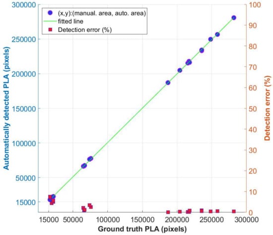
Figure 20.
Visual representation of the automatically detected (experimental) and ground truth (manual) area for plants A to E in the 4-week experiment. The points depicted in the figure as blue circles represent the two different image data points (manual vs. automated plant area calculation) for the same plant, each time. The green line represents the best linear fit to this dataset. The small red squares represent the percentage (%) detection error in the manual and automatic areas for each case.
To summarize, the outcomes of both tests are considered adequate for the realization of plant detection and localization in the context of plant photography. Moreover, the mechanical structural margin of error detected in the system’s accuracy and repeatability evaluation test is viewed as satisfactory, and we are confident that this degree of inaccuracies will not impede the operational efficiency of our system in practical, real-world situations. Furthermore, the experiments revealed a consistently smooth linear motion of the carriage. This observation confirms a well-designed experimental system that is properly assembled, which minimizes the risk of missing steps from the chosen stepper motor (i.e., the motor possesses adequate torque for the load). It also highlights a precise selection of initialization parameters for the stepper motor driver in the programming (maximum speed = 500 out of 1300, acceleration = 500 out of 20,000, microstepping resolution = 2). Also, the installed LEDs were successful in providing adequate illumination for the plants during image capture throughout the entire process. Furthermore, the inclusion of limit switches beneath the carriage not only improves the current level of precision but also adds an extra layer of safety at the far ends of the beam. This ensures that the “home” position is accurately identified before every initialization startup process. Considering the test outcomes and the overall system performance, it has been ascertained that no corrective actions need to be taken, apart from periodic maintenance, which is essential for all mechanical systems with moving components (e.g., fastening of the timing belt, leveling, inspection of the alignment of the carriage’s wheels to ensure their proper positioning, etc.). The attained degree of precision in motion is considered adequate for the intended purpose of capturing plant images for research experimentation, which is the main purpose of the current application. Additionally, the inclusion of the “Autofind” feature in our system provides an extra advantage (explained thoroughly in Section 2.2.4). In cases where the user’s initial plant number set for identification is ultimately unsuccessful (e.g., less plants were identified), this feature activates the LED strip to flash, notifying the user of the problem. In this case, the user has the ability to reset the alarm using the graphical menu and carry out preventive actions. The plant features collected by the automated linear robotic camera system proposed in this work, not only provide the potential for individual plant monitoring, but also facilitate the comparison of growth patterns across various environments.
3.4. Limitations, Future Outlooks, and Related Studies
Although the proposed system in this work has been shown to be accurate and efficient for its dedicated task tailored to plant photography for research purposes, there are still limitations that we need to consider. One limitation is that the images can only be acquired from the top view, indicating that the error may increase in the scenario where the foliage of neighboring plants partially overlaps. Even though there was no specific requirement for such an arrangement, a common assumption scenario observed in many growth monitoring and phenotyping analysis systems is the spacing of planting beds or the arrangement of pots in a photographical scene, ensuring sufficient distance between them, as, for example, in [4,25]. In other words, and specifically for our scenario, the five (or six) pots in each row were randomly positioned with sufficient spacing to prevent any overlap of foliage, even when the plants reached their full growth. However, future research endeavors will encompass cases where mature plants exhibit partially overlapping foliage, as the adjacent leaves’ segmentation control presents a promising and challenging aspect for the successful identification of plants in a general scenario [3]. Furthermore, future studies will organize dedicated and expanded experiments on a broader field of research to further test our system and to continue to collect images captured in its permanent installation place, that is, the greenhouse. One further limitation is the existing system’s ability to recognize and manage only a single plant at a time in a sequential manner, rather than processing multiple plants simultaneously, as demonstrated in [6,16,17,18], for example. Nevertheless, despite its usefulness and potential time-saving benefits, no such limitation existed for the detection of numerous plants and time-related concerns during our design phase. However, since to simultaneously manage multiple plants seems a necessary augmentation, we are currently implementing an algorithmic pipeline towards lettuce plant detection and localization on a panorama image, which is created by combing multiple overlapping images together (image stitching), captured from our system.
The results obtained from the conducted experiments clearly indicate that our linear robotic camera is capable of effectively identifying mature plants. Nevertheless, there is room for improvement, which could be achieved by incorporating a higher resolution binocular field stereo system. This parallel adaptation would greatly facilitate the investigation procedures and enable the detection of even the most intricate contours within the projected leaf area, including those that are exceptionally small. The selection of the current stereo camera module was based on its synchronization capabilities, as well as its similarities in characteristics and features to both RGB and IR cameras, as mentioned earlier. In this research, the calibration of the stereo system was extensively discussed, and the IR images were efficiently captured, stored in dedicated folders, and synchronized along with the colored images and datalogging information. However, the primary focus was on the task of plant recognition and localization, which was accomplished using the RGB camera and simple image processing techniques. Consequently, both images representing the same scene are readily available and can be further processed using image registration techniques to derive the relevant Normalized Difference Vegetation Index (NDVI) of the plants, which provides valuable information about their health status. Nevertheless, the calculations associated with the NDVI are reserved for future endeavors.
Moreover, as an ongoing project, our experimental plans include the incorporation of different imaging modalities, namely hyperspectral imaging in parallel investigations of different yet interesting image acquisition angle views, other than the top- or side-view imaging modes [41]. This approach, along with the simultaneous utilization of instruments such as the Konica’s Minolta SPAD-502 m and other affordable alternatives already in-house developed [61], which are employed for assessing plant health by analyzing their relative chlorophyll content, will permit the methods presented here to be incorporated into a broader field of research for plant growth monitoring.
We are of the opinion that there is room for enhancing the user friendliness of this system and expanding its applicability to a wider range of users. Our objective is not to encompass every conceivable plant species, but rather to establish a system that can be easily expanded and adapted to meet evolving needs. To this end, we are currently developing an enhanced iteration of our system. Our ongoing efforts involve expanding our robotic camera positioning system to function as a Cartesian robot. This advancement will enable us to cover a larger area and grant the camera platform the freedom to be positioned at any point within the x–y coordinate system, specifically above the crop canopy.
The utilization of small-scale robotic machines or CNC-based mechanization techniques in agricultural operations, as demonstrated in similar published works, as for example, in [4,14,25,38], showcases the effectiveness of employing Cartesian robots to address the issue of precise movement and among others, to cover a wider area of plants in the investigation, a fact that possesses a design advantage over our current system’s implementation. However, this can be achieved either by programming the cameras to move in stable increments and to stop at specific locations to acquire images [14], or through the establishment of predetermined coordinates and predefined targets [25,38], or even manually operating them to stop at specific locations to acquire images [4]. The image capturing and processing device, for example, as presented in [4], although interesting in its implementation, is entirely manually operated by a user. This user must utilize a toggle switch each time to maneuver the system forward or backward along the track for image data collection and the subsequent crop status monitoring. Our proposed system differs significantly from conventional manual practices, since it can operate autonomously, with minor user interaction. Furthermore, it features automatic identification, localization, and image capturing of the plants being analyzed, thus alleviating the burden of plant photography for human photographers and crop researchers. Moreover, in contrast to approaches that rely on fixed spaces or specific plant locations, as compared to the solutions presented in [14,25,38], the linear robotic camera system developed in this study continuously scans a row of target plants and accurately detects and localizes the plants themselves using simple image processing techniques and OpenCV primitives. This system allows users the flexibility to position the targeted plants in any desired arrangement inside a row, with the robot seamlessly adjusting to the new configuration. This facilitates a more efficient utilization of the typically limited space within a small greenhouse.
4. Conclusions
The current investigation introduces a new, cost-effective, one-degree-of-freedom linear robotic camera system for automatic plant photography. The system is specifically designed for the automatic and systematic identification and localization of plants ordered in a row, in a complete random design, which can thus can readily facilitate the greenhouse’s plant growth monitoring procedures. The entire system was meticulously constructed using readily available materials, parts, and basic electronic components. The primary objective of this study was to offer comprehensive information about the hardware components used, the software pipeline, and the implementation details of the proposed system. A preliminary assessment of the experimental prototype, conducted on a small sample of lettuce plants primarily in laboratory settings, demonstrated encouraging outcomes in terms of plant identification and localization. Although the measurements presented were performed on one type of lettuce plant, we believe that our device can perform just as well with various kinds of plants and in similar applications with minor modifications. Among other things, our device will be useful for creating custom image datasets useful for conducting testing and experimentation, while developing computer vision algorithms.
The system was designed and developed by a team of engineers from various disciplines (electronic, computer, and agricultural engineers) to fulfill realistic needs for automatic plant growth monitoring and imaging in an educational greenhouse. The length and height dimensions of the whole construction were chosen so as to align with the crop rows in the greenhouse, ensuring seamless monitoring and imaging processes without disrupting the existing infrastructure. The agricultural engineers, apart from the description of the problem and the initial technical requirements, also closely followed the progress of the implementation, evaluating the intermediate results and intervening with timely observations in the design decisions that were taken. This collaborative approach was continued during the whole development process and extended to both hardware and software development, so a device corresponding to the initial requirements was produced. The same procedure was followed for the evaluation of the construction’s operation to monitor the growth of illustrative lettuce samples, feeding back the design and implementation phase with new data that were incorporated into the device. Several such cycles of agile development needed to take place before the device started to operate as required.
Such a device is in line with the requirements of Industry 4.0 for smart agriculture, known as Agriculture 4.0, as it can contribute to the automation and modernization of agricultural production. Agriculture 4.0 refers to the anticipated radical changes in agricultural production through the application of recent advances in information technology. Agriculture 4.0 is a term for the next big trends to impact this industry, including a greater focus on precision agriculture with the regular application of the Internet of Things, autonomous robots, big-data, and artificial intelligence to drive greater business efficiencies, make smarter planning decisions, and lower the environmental footprint. Labor-intensive tasks will be undertaken by autonomous ground robots or unmanned aerial vehicles equipped with machine vision systems and precision telemetry. With Agriculture 4.0, the whole agri-food chain will become more competitive and profitable, as deeper insights and precise advice for plant requirements will empower farmers to minimize agricultural input (water, nutrients, plant protection, etc.), thus minimizing environmental and health hazards, but also to scale production further by reducing space requirements, growing periods, and logistic chains [62]. Devices such as the one presented here are a perfect fit towards this direction for the future, Internet-based agriculture, as it can provide farmers and agronomists with valuable remote monitoring of crop production and decision support, so critical decisions for crop growth and health are made on time. Our future plans include the in vivo evaluation of our prototype in the greenhouse, with various kinds of plants, to assure its performance in real conditions. The next milestone includes the generalization of this prototype to the two and the three dimensions, so it can cover larger surfaces and vertical farming, respectively, with almost the same robotic head, eliminating the need for one such device per row in a greenhouse.
Author Contributions
Conceptualization, Z.K., S.P. (Spyros Perdikakis), I.N.D. and S.P. (Spyros Panagiotakis); methodology, Z.K. and S.P. (Spyros Perdikakis); software, Z.K. and S.P. (Spyros Perdikakis); validation, Z.K., S.P. (Spyros Perdikakis) and S.P. (Spyros Panagiotakis); formal analysis, Z.K.; investigation, Z.K., S.P. (Spyros Perdikakis), I.N.D. and D.M.P.; resources, Z.K., S.P. (Spyros Perdikakis) and D.M.P.; data curation, Z.K.; writing—original draft preparation, Z.K. and S.P. (Spyros Perdikakis); writing—review and editing, Z.K., S.P. (Spyros Perdikakis), I.N.D., D.M.P. and S.P. (Spyros Panagiotakis); visualization, Z.K.; supervision, Z.K., I.N.D. and S.P. (Spyros Panagiotakis); project administration, Z.K., I.N.D. and S.P. (Spyros Panagiotakis); funding acquisition, Z.K., S.P. (Spyros Perdikakis), I.N.D. and S.P. (Spyros Panagiotakis). All authors have read and agreed to the published version of the manuscript.
Funding
This research received no external funding.
Data Availability Statement
The data used to support this study’s findings are available from the corresponding authors upon logical request.
Acknowledgments
This work was partially supported by Hellenic Mediterranean University internal funds in the framework of a two-year postdoctoral fellowship “Multispectral image processing for the creation of a data collection and processing system with application in Precision Agriculture”, awarded to the first corresponding author. Also, the authors acknowledge partial financial support from the European Union and Greek national funds through the Operational Program Competitiveness, Entrepreneurship and Innovation, under the call RESEARCH-CREATE-INNOVATE (project SOilless culture UPgrade—SOUP code: T1EDK-04171).
Conflicts of Interest
The authors declare no conflicts of interest. The funders had no role in the design of the study; in the collection, analyses, or interpretation of data; in the writing of the manuscript; or in the decision to publish the results.
Appendix A
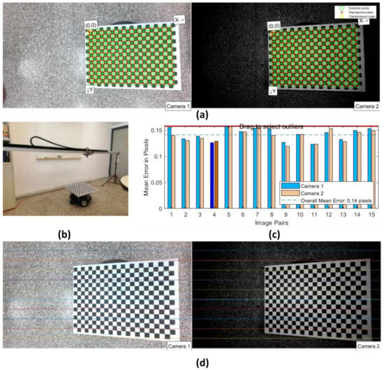
Figure A1.
View of checkerboard pattern (x-direction along the longer side). In (a), the detected points are shown in green circles and the reprojected points with red crosses. In (b), the robotic platform used for the checkerboard mount is shown. In (c), the reprojection error for the 15 pair images is shown. In (d), an example of two images after the rectification procedure is shown. The checkerboard image pair example shown corresponds to the highlighted 1st pair of the 30-image dataset in figure (c) (colored figure online).
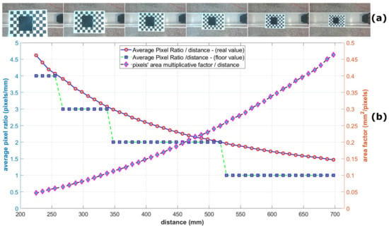
Figure A2.
In (a), we show some of the RGB images captured at various positions of the sample object with known dimensions (total of 48 different positions measured in the range 225 to 700 mm, with increments of 1 cm). By manually analyzing the object in all these images, the scale (pixels/mm) as well as the factor mm2/pixels along various distances/depths can be calculated (b). Considering the left y-axis, the average pixel ratio (pixels/mm) for each distance is shown as real valued (small red circles in the upper plot) and rounded down (blue squares in the lower plot) points. The ratio was computed manually on each image by measuring both known sides of the test object at various distances (depths). On the right y-axis of the same figure, a pixel’s multiplicative factor () against the same distance axis is shown as magenta diamonds. (colored figure online).
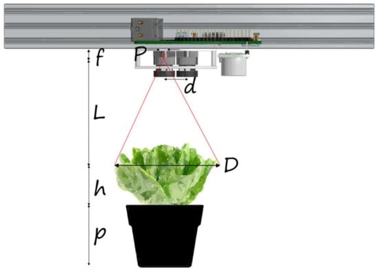
Figure A3.
Calculation of plant’s width (maximum diameter) using triangulation (similar triangles principle). The letter P denotes the plant’s width as it appears on the RGB imaging sensor, where the letter f stands for the focal length of the camera (in mm), and the letter D is the actual plant’s width (in mm). The letter L represents the distance from the camera and the sensors. The letter h denotes the plant’s height, p the pot’s height, and d the distance between the cameras.

Table A1.
List of materials and components.
Table A1.
List of materials and components.
| Item # | Component | Short Usage Description | Quantity |
|---|---|---|---|
| 1 | Camera tripod | Whole structure support | 2 |
| 2 | V-Slot 2060 1000 mm: natural anodized | Horizontal support for the carriage | 2 |
| 3 | V-Slot 2060 1500 mm: natural anodized | Horizontal support for the carriage | 1 |
| 4 | Cable drag chain 10 × 10 mm (m) | Cable management | 3 |
| 5 | Drag/cable chain mounting bracket | - | 1 |
| 6 | Aluminum 248 × 40 × 2 mm | Cable drag chain support | 2 |
| 7 | Double tee nut | V-slot assembly | 14 |
| 8 | Spring-loaded tee nuts | V-slot assembly | 10 |
| 9 | Stepper Motor Driver TMC2209 V2.0 | - | 1 |
| 10 | Plywood 250 × 150 × 6 mm | Carriage support | 1 |
| 11 | V-Slot Gantry Set 2020 × 2080 Xtreme | For the movement of the carriage | 1 |
| 12 | Stepper motor 2.8 kg.cm 42BYGHW208 | - | 1 |
| 13 | Timing belt: GT2 (m) | - | 4 |
| 14 | Aluminum GT2 timing pulley: 12T—5 mm | Toothed pulley for the precise movement of the carriage | 1 |
| 15 | Power Supply 12 V 2 A: output 5.5 × 2.1 PSU-1602 | - | 1 |
| 16 | Power supply 5 V 3 A for Raspberry Pi 4 | - | 1 |
| 17 | Raspberry Pi 4-Model B-8 GB | - | 1 |
| 18 | Raspberry Pi 4 B Heatsink: black (set of 3) | RPi 4B cooling | 1 |
| 19 | DC Fan 50 × 50 × 10 mm 12 V: MagLev | RPi 4B cooling | 1 |
| 20 | Memory card microSDHC 64 GB Class 10: SanDisk Ultra | RPi 4B OS and programming | 1 |
| 21 | Microswitch Mini SPDT ON-(ON): with roller lever | Determination of the two ends of the carriage | 2 |
| 22 | Adafruit Time-of-Flight (ToF) sensor VL53L0X | - | 1 |
| 23 | Humidity and temperature sensor (AM2301) | Temperature, humidity | 1 |
| 24 | GPIO Header for Raspberry Pi 2 × 20 stackable | - | 1 |
| 25 | infrared LED board | Illuminates the plants in the infrared spectrum | 2 |
| 26 | Arducam stereo USB camera, synchronized, 2MP 1080P | RGB and IR images capture | 1 |
| 27 | PCB board electronics and other components | JST XH Connectors (2 pin/3 pin/4 pin), P2N222ANPN Transistor, resistors, capacitors, Relay DPDT 5 V, 1N4007 Diode, cables, multi-socket, bolts, nuts, washers, screws, cable insulation, etc. | 1 |

Table A2.
Stereo camera calibration parameters.
Table A2.
Stereo camera calibration parameters.
| Camera | Calibration Parameters | Equation | Calculated Values |
|---|---|---|---|
| RGB NIR | Intrinsic parameters * | ||
| RGB NIR | Radial distortions | ||
| RGB NIR | Tangential distortions | ] ] | |
| RGB NIR | Rotation of RGB camera relative to NIR camera | ||
| RGB NIR | Translation of RGB camera relative to NIR camera ** |
* units in pixels, ** units in mm, , , and x,y: location of undistorted pixels (measureless).
References
- Ehret, D.; Lau, A.; Bittman, S.; Lin, A.; Tim Shelford, T. Automated monitoring of greenhouse crops. Agronomie 2001, 21, 403–414. [Google Scholar] [CrossRef]
- Li, H.; Guo, Y.; Zhao, H.; Wang, Y.; Chow, D. Towards automated greenhouse: A state of the art review on greenhouse monitoring methods and technologies based on internet of things. Comput. Electron. Agric. 2021, 191, 106558. [Google Scholar] [CrossRef]
- Li, L.; Zhang, Q.; Huang, D. A review of imaging techniques for plant phenotyping. Sensors 2014, 14, 20078–20111. [Google Scholar] [CrossRef] [PubMed]
- Chang, C.-L.; Chung, S.-C.; Fu, W.-L.; Huang, C.-C. Artificial intelligence approaches to predict growth, harvest day, and quality of lettuce (Lactuca sativa L.) in a IoT-enabled greenhouse system. Biosyst. Eng. 2021, 212, 77–105. [Google Scholar] [CrossRef]
- Sishodia, R.P.; Ray, R.L.; Singh, S.K. Applications of Remote Sensing in Precision Agriculture: A Review. Remote Sens. 2020, 12, 3136. [Google Scholar] [CrossRef]
- Ma, J.; Li, Y.; Chen, Y.; Du, K.; Zheng, F.; Zhang, L.; Sun, Z. Estimating above ground biomass of winter wheat at early growth stages using digital images and deep convolutional neural network. Eur. J. Agron. 2019, 103, 117–129. [Google Scholar] [CrossRef]
- Zhang, L.; Xu, Z.; Xu, D.; Ma, J.; Chen, Y.; Fu, Z. Growth monitoring of greenhouse lettuce based on a convolutional neural network. Hortic. Res. 2020, 7, 124. [Google Scholar] [CrossRef] [PubMed]
- Sladojevic, S.; Arsenovic, M.; Anderla, A.; Culibrk, D.; Stefanovic, D. Deep Neural Networks Based Recognition of Plant Diseases by Leaf Image Classification. Comput. Intell. Neurosci. 2016, 2016, 3289801. [Google Scholar] [CrossRef] [PubMed]
- Too, E.C.; Yujian, L.; Njuki, S.; Yingchun, L. A comparative study of fine-tuning deep learning models for plant disease identification. Comput. Electron. Agric. 2019, 161, 272–279. [Google Scholar] [CrossRef]
- Reyes, A.K.; Caicedo, J.C.; Camargo, J.E. Fine-tuning Deep Convolutional Networks for Plant Recognition. Conf. Labs Eval. Forum 2015, 1391, 467–475. [Google Scholar]
- Rahnemoonfar, M.; Sheppard, C. Deep Count: Fruit Counting Based on Deep Simulated Learning. Sensors 2017, 17, 905. [Google Scholar] [CrossRef]
- Fuentes-Peñailillo, F.; Carrasco Silva, G.; Pérez Guzmán, R.; Burgos, I.; Ewertz, F. Automating Seedling Counts in Horticulture Using Computer Vision and AI. Horticulturae 2023, 9, 1134. [Google Scholar] [CrossRef]
- Kuwata, K.; Shibasaki, R. Estimating crop yields with deep learning and remotely sensed data. In Proceedings of the 2015 IEEE International Geoscience and Remote Sensing Symposium (IGARSS), Milan, Italy, 26–31 July 2015; pp. 858–861. [Google Scholar]
- Rajalakshmi, T.S.; Panikulam, P.; Sharad, P.K.; Nair, R.R. Development of a small scale cartesian coordinate farming robot with deep learning based weed detection. J. Phys. Conf. Ser. 2021, 1969, 012007. [Google Scholar] [CrossRef]
- Chen, C.-J.; Huang, Y.-Y.; Li, Y.-S.; Chang, C.-Y.; Huang, Y.-M. An AIoT Based Smart Agricultural System for Pests Detection. IEEE Access 2020, 8, 180750–180761. [Google Scholar] [CrossRef]
- Hamidon, M.H.; Ahamed, T. Detection of Defective Lettuce Seedlings Grown in an Indoor Environment under Different Lighting Conditions Using Deep Learning Algorithms. Sensors 2023, 23, 5790. [Google Scholar] [CrossRef]
- Li, Z.; Li, Y.; Yang, Y.; Guo, R.; Yang, J.; Yue, J.; Wang, Y. A high-precision detection method of hydroponic lettuce seedlings status based on improved Faster RCNN. Comput. Electron. Agric. 2021, 182, 106054. [Google Scholar] [CrossRef]
- Franchetti, B.; Pirri, F. Detection and Localization of Tip-Burn on Large Lettuce Canopies. Front. Plant Sci. 2022, 13, 874035. [Google Scholar] [CrossRef] [PubMed]
- Vilani Sachithra, V.; Subhashini, L.D.C.S. How artificial intelligence uses to achieve the agriculture sustainability: Systematic review. Artif. Intell. Agric. 2023, 8, 46–59. [Google Scholar] [CrossRef]
- Tian, H.; Wang, T.; Liu, Y.; Qiao, X.; Li, Y. Computer vision technology in agricultural automation—A review. Inf. Process. Agric. 2020, 7, 1–19. [Google Scholar] [CrossRef]
- Adli, H.K.; Remli, M.A.; Wan Salihin Wong, K.N.S.; Ismail, N.A.; González-Briones, A.; Corchado, J.M.; Mohamad, M.S. Recent Advancements and Challenges of AIoT Application in Smart Agriculture: A Review. Sensors 2023, 23, 3752. [Google Scholar] [CrossRef]
- Mavridou, E.; Vrochidou, E.; Papakostas, G.A.; Pachidis, T.; Kaburlasos, V.G. Machine Vision Systems in Precision Agriculture for Crop Farming. J. Imaging 2019, 5, 89. [Google Scholar] [CrossRef] [PubMed]
- Dhanya, V.G.; Subeesh, A.; Kushwaha, N.L.; Vishwakarma, D.K.; Kumar, T.N.; Ritika, G.; Singh, A.N. Deep learning based computer vision approaches for smart agricultural applications. Artif. Intell. Agric. 2022, 6, 211–229. [Google Scholar] [CrossRef]
- Kamilaris, A.; Prenafeta-Boldú, F.X. Deep learning in agriculture: A survey. Comput. Electron. Agric. 2018, 147, 70–90. [Google Scholar] [CrossRef]
- Yeh, Y.H.F.; Lai, T.C.; Liu, T.Y.; Liu, C.C.; Chung, W.C.; Lin, T.T. An automated growth measurement system for leafy vegetables. Biosyst. Eng. 2014, 117, 43–50. [Google Scholar] [CrossRef]
- Yang, R.; Wu, Z.; Fang, W.; Zhang, H.; Wang, W.; Fu, L.; Majeed, Y.; Li, R.; Cui, Y. Detection of abnormal hydroponic lettuce leaves based on image processing and machine learning. Inf. Process. Agric. 2021, 10, 1–10. [Google Scholar] [CrossRef]
- Abbasi, R.; Martinez, P.; Ahmad, R. Automated Visual Identification of Foliage Chlorosis in Lettuce Grown in Aquaponic Systems. Agriculture 2023, 13, 615. [Google Scholar] [CrossRef]
- Yang, C.I.; Hsieh, K.W.; Tsai, C.Y.; Huang, Y.I.; Chen, L.Y.; Chen, S. Development of an automation system for greenhouse seedling production management using radio-frequency-identification and local remote sensing techniques. Eng. Agric. Environ. Food 2014, 7, 52–58. [Google Scholar] [CrossRef]
- Wang, L.; Duan, Y.; Zhang, L.; Rehman, T.U.; Ma, D.; Jin, J. Precise Estimation of NDVI with a Simple NIR Sensitive RGB Camera and Machine Learning Methods for Corn Plants. Sensors 2020, 20, 3208. [Google Scholar] [CrossRef] [PubMed]
- Wäldchen, J.; Mäder, P. Plant Species Identification Using Computer Vision Techniques: A Systematic Literature Review. Arch. Comput. Methods Eng. 2017, 25, 507–543. [Google Scholar] [CrossRef] [PubMed]
- Xie, D.; Chen, L.; Liu, L.; Chen, L.; Wang, H. Actuators and Sensors for Application in Agricultural Robots: A Review. Machines 2022, 10, 913. [Google Scholar] [CrossRef]
- Wang, T.; Chen, B.; Zhang, Z.; Li, H.; Zhang, M. Applications of machine vision in agricultural robot navigation: A review. Comput. Electron. Agric. 2022, 198, 107085. [Google Scholar] [CrossRef]
- Story, D.; Kacira, M. Design and implementation of a computer vision-guided greenhouse crop diagnostic system. Mach. Vis. Appl. 2015, 26, 495–506. [Google Scholar] [CrossRef]
- Moraitis, M.; Vaiopoulos, K.; Balafoutis, A.T. Design and Implementation of an Urban Farming Robot. Micromachines 2022, 13, 250. [Google Scholar] [CrossRef] [PubMed]
- Thomopoulos, V.; Bitas, D.; Papastavros, K.-N.; Tsipianitis, D.; Kavga, A. Development of an Integrated IoT-Based Greenhouse Control Three-Device Robotic System. Agronomy 2021, 11, 405. [Google Scholar] [CrossRef]
- Birrell, S.; Hughes, J.; Cai, J.Y.; Iida, F. A field-tested robotic harvesting system for iceberg lettuce. J. Field Robot. 2019, 37, 225–245. [Google Scholar] [CrossRef] [PubMed]
- Amer, M.A.; Rajan, P.; Mehanny, S.; Artyszak, A.; Ahmed, M.A.A. Innovative Design of an Experimental Jasmine Flower Automated Picker System Using Vertical Gripper and YOLOv5. Agriculture 2023, 13, 1595. [Google Scholar] [CrossRef]
- Kautsar, S.; Rosdiana, E.; Widiawan, B.; Setyohadi, D.P.S.; Riskiawan, H.Y.; Firgiyanto, R. Farming Bot: Precision Agriculture System in Limited Land Based On Computer Numerical Control (CNC). IOP Conf. Ser. Earth Environ. Sci. 2020, 411, 012059. [Google Scholar] [CrossRef]
- Lauretti, C.; Zompanti, A.; Sara Cimini, S.; De Gara, L.; Marco Santonico, M.; Zollo, L. A low-cost multispectral device for in-field fruit ripening assessment. IEEE Sens. J. 2023. [Google Scholar] [CrossRef]
- Noguera, M.; Millan, B.; Andújar, J.M. New, Low-Cost, Hand-Held Multispectral Device for In-Field Fruit-Ripening Assessment. Agriculture 2023, 13, 4. [Google Scholar] [CrossRef]
- Zhang, L.; Maki, H.; Ma, D.; Sánchez-Gallego, J.A.; Mickelbart, M.V.; Wang, L.; Rehman, T.U.; Jin, J. Optimized angles of the swing hyperspectral imaging system for single corn plant. Comput. Electron. Agric. 2019, 156, 349–359. [Google Scholar] [CrossRef]
- GRobotronics. V-Slot 2060 1500 mm-Natural Anodized. Available online: https://grobotronics.com/v-slot-2060-1500mm-natural-anodized.html (accessed on 10 June 2022).
- v-store.gr. Camera Tripod. Available online: https://v-store.gr/el/tripoda/u230254-tripodo-megalo-epekteinomeno-megistoy-ypsoys-210cm-p-7947.html (accessed on 10 June 2022).
- GRobotronics. V-Slot Gantry Plate 20 mm–80 mm Set. Available online: https://grobotronics.com/v-slot-gantry-plate-20mm-80mm-set.html (accessed on 10 June 2022).
- GRobotronics. Stepper Motor 2.8 kg·cm (200 step/rev) 42BYGHW298. Available online: https://grobotronics.com/stepper-motor-42byghw208-2.6kg.cm.html (accessed on 10 June 2022).
- GRobotronics. Stepper Motor Driver TMC2209 V2.0. Available online: https://grobotronics.com/stepper-motor-driver-tmc2209-v2.0.html (accessed on 10 June 2022).
- GRobotronics. Microswitch Mini SPDT ON-(ON)-with Roller Lever. Available online: https://grobotronics.com/microswitch-mini-spdt-on-on-with-roller-lever.html (accessed on 10 June 2022).
- Arducam. Arducam Stereo USB Camera, Synchronized Visible Light and Infrared Camera, 2MP 1080P Day and Night Mini UVC USB2.0 Webcam Board for Face Recognition and Biological Detection. Available online: https://www.uctronics.com/arducam-stereo-usb-camera-synchronized-visible-light-and-infrared-camera-2mp-1080p-day-and-night-mini-uvc-usb2-0-webcam-board-for-face-recognition-and-biological-detection.html (accessed on 14 June 2022).
- OMNIVISION. OV2710-1E Datasheet. Available online: https://www.ovt.com/products/ov02710-a68a-1e/ (accessed on 14 June 2022).
- GRobotronics. Infrared Led Board. Available online: https://grobotronics.com/infrared-led-board-pack-of-2.html (accessed on 20 June 2022).
- GRobotronics. Adafruit VL53L0X Time of Flight Distance Sensor- ~30 mm to 1000 mm. Available online: https://grobotronics.com/adafruit-vl53l0x-time-of-flight-distance-sensor-30-to-1000mm.html (accessed on 12 July 2022).
- GRobotronics. Ultrasonic Sensor—Ranging Detector 2–400 cm HC-SR04. Available online: https://grobotronics.com/ultrasonic-sensor-sr04.html (accessed on 12 July 2022).
- GRobotronics. Raspberry Pi 4 - Model B - 8 GB. Available online: https://grobotronics.com/raspberry-pi-4-model-b-8gb.html (accessed on 10 June 2022).
- Arducam. Datasheet OV2710 Dual-Lens Camera Module. Available online: https://www.uctronics.com/download/Amazon/B0198_Datasheet.pdf (accessed on 14 June 2022).
- Computer Vision User Interface (cvui). Available online: https://dovyski.github.io/cvui/ (accessed on 10 December 2022).
- Arvidsson, S.; Pérez-Rodríguez, P.; Mueller-Roeber, B. A growth phenotyping pipeline for Arabidopsis thaliana integrating image analysis and rosette area modeling for robust quantification of genotype effects. New Phytol. 2011, 191, 895–907. [Google Scholar] [CrossRef] [PubMed]
- Walter, A.; Scharr, H.; Gilmer, F.; Zierer, R.; Nagel, K.A.; Ernst, M.; Wiese, A.; Virnich, O.; Christ, M.M.; Uhlig, B.; et al. Dynamics of seedling growth acclimation towards altered light conditions can be quantified via GROWSCREEN: A setup and procedure designed for rapid optical phenotyping of different plant species. New Phytol. 2007, 174, 447–455. [Google Scholar] [CrossRef] [PubMed]
- Jansen, M.; Gilmer, F.; Biskup, B.; Nagel, K.A.; Rascher, U.; Fischbach, A.; Briem, S.; Dreissen, G.; Tittmann, S.; Braun, S.; et al. Simultaneous phenotyping of leaf growth and chlorophyll fluorescence via GROWSCREEN FLUORO allows detection of stress tolerance in Arabidopsis thaliana and other rosette plants. Funct. Plant Biol. 2009, 36, 902–914. [Google Scholar] [CrossRef] [PubMed]
- Minervini, M.; Abdelsamea, M.M.; Tsaftaris, S.A. Image-Based plant phenotyping with incremental learning and active contours. Ecol. Inform. 2013, 23, 35–48. [Google Scholar] [CrossRef]
- De Vylder, J.; Vandenbussche, F.; Hu, Y.; Philips, W.; Van Der Straeten, D. Rosette tracker: An open source image analysis tool for automatic quantification of genotype effects. Plant Physiol. 2012, 160, 1149–1159. [Google Scholar] [CrossRef]
- Kamarianakis, Z.; Panagiotakis, S. Design and Implementation of a Low-Cost Chlorophyll Content Meter. Sensors 2023, 23, 2699. [Google Scholar] [CrossRef]
- Advances in Agriculture 4.0. Available online: https://www.mdpi.com/journal/futureinternet/special_issues/A_IA4 (accessed on 4 April 2024).
Disclaimer/Publisher’s Note: The statements, opinions and data contained in all publications are solely those of the individual author(s) and contributor(s) and not of MDPI and/or the editor(s). MDPI and/or the editor(s) disclaim responsibility for any injury to people or property resulting from any ideas, methods, instructions or products referred to in the content. |
© 2024 by the authors. Licensee MDPI, Basel, Switzerland. This article is an open access article distributed under the terms and conditions of the Creative Commons Attribution (CC BY) license (https://creativecommons.org/licenses/by/4.0/).