Abstract
We develop the online process parameter design (OPPD) framework for efficiently handling streaming data collected from industrial automation equipment. This framework integrates online machine learning, concept drift detection and Bayesian optimization techniques. Initially, concept drift detection mitigates the impact of anomalous data on model updates. Data without concept drift are used for online model training and updating, enabling accurate predictions for the next processing cycle. Bayesian optimization is then employed for inverse optimization and process parameter design. Within OPPD, we introduce the online accelerated support vector regression (OASVR) algorithm for enhanced computational efficiency and model accuracy. OASVR simplifies support vector regression, boosting both speed and durability. Furthermore, we incorporate a dynamic window mechanism to regulate the training data volume for adapting to real-time demands posed by diverse online scenarios. Concept drift detection uses the EI-kMeans algorithm, and the Bayesian inverse design employs an upper confidence bound approach with an adaptive learning rate. Applied to single-crystal fabrication, the OPPD framework outperforms other models, with an RMSE of 0.12, meeting precision demands in production.
1. Introduction
With the advancement of computer technology and increased computational capabilities, the field of machine learning has had a profound impact on industry, particularly within the context of Industry 4.0 [1]. Industry 4.0 standards encourage the use of intelligent sensors, devices and machinery, enabling smart factories to continuously collect data relevant to production. By processing the gathered data, machine learning techniques can generate executable intelligence, thereby improving production efficiency without significantly altering the required resources [2]. Traditional machine learning [3] is typically associated with offline machine learning, also known as batch machine learning. It involves training on historical data to obtain machine learning models. To update the model, it is necessary to retrain it on a new dataset. In contrast, online machine learning refers to the process of continuously training and dynamically updating models as data stream in. This approach allows models to track changes in data in real time, leading to improved predictive performance [4].
In the era of Industry 4.0, the level of automation and informatization of equipment is exceptionally high. Devices are equipped with sensors that enable real-time monitoring of equipment parameters, with the collected data being sent back to monitoring databases, resulting in a continuous stream of data. In the context of streaming data [5], online machine learning addresses the limitation of offline machine learning, which cannot update models in real time. This capability can significantly enhance the accuracy of model predictions. Consequently, online machine learning exhibits unique advantages in industrial applications. Currently, while there is some research in the field of online machine learning, its application in the industrial domain remains relatively limited. The primary challenges [6] include:
- (1)
- Computational efficiency of algorithms: Currently, there are numerous online incremental algorithms, such as online decision tree models and incremental clustering algorithms. These algorithms require setting hyperparameters based on different streaming data. In contrast, online support vector regression models do not necessitate this prior knowledge. Ma et al. proposed accurate online support vector regression, also abbreviated as AONSVR [7]. However, this method exhibits high computational complexity, making it unsuitable for meeting the rapid computation requirements of industrial applications. Subsequent researchers have made various improvements to AONSVR [8,9,10], but their primary focus has been on enhancing predictive accuracy, without in-depth investigation into the computational performance of the model. The ORSVR approach introduced by Yu has improved computational performance but obtains a lower predictive accuracy than AONSVR because of its robustness. Therefore, it is essential to enhance computational speed while maintaining predictive accuracy.
- (2)
- Concept drift detection [11]: Concept drift is a phenomenon in which the statistical properties of a target domain change over time in an arbitrary way [12]. In online machine learning, where the model is trained on each streaming data point, the model tends to update in the wrong direction gradually when data undergo concept drift. As a result, it is crucial to monitor the streaming data. Concept drift detection algorithms perform real-time monitoring of the data distribution in streaming data. When drift is detected, that portion of data is discarded and it is not used for model training. The system can then issue an alert for human intervention or other necessary actions to address the concept drift.
To overcome the challenges outlined above, this paper introduces an online processing parameter prediction and design framework that integrates online machine learning, concept drift detection and Bayesian optimization. The primary contributions of this paper are as follows:
- (1)
- A revolutionary framework optimizes dynamic industrial processes through dynamic machine learning. A framework for online processing parameters design and design in industrial applications is introduced. The framework integrates online machine learning for prediction, concept drift detection and reverse design based on Bayesian optimization. It is capable of addressing dynamic scenarios that require tasks such as drift detection in equipment processing data, dynamic performance prediction and the online optimization and design of equipment processing parameters.
- (2)
- Innovative OASVR model for dynamic industrial efficiency. To meet the rapid computation demands of industrial environments, we introduce the online accelerated support vector regression (OASVR) model. OASVR decomposes the original problem of online support vector regression into two smaller quadratic programming problems, resulting in more than a 2× improvement in computational speed while maintaining a prediction accuracy similar to the classic AONSVR algorithm. Additionally, we incorporate the EI-kMeans algorithm for concept drift detection in streaming data, further ensuring the accuracy of the model predictions.
- (3)
- OASVR outperforms mainstream algorithms in single-crystal growth applications. The OASVR algorithm introduced in this paper has demonstrated excellent results when applied to a dataset on the growth of single crystals. It outperforms other mainstream online incremental learning algorithms. By using an adaptive learning rate maximum upper bound function in the Bayesian optimization acquisition function, the algorithm strikes a balance between exploration and exploitation. The root mean square error (RMSE) between the predictive recommendations of the algorithm and actual experimental results is only 0.12, meeting the stringent requirements of production standards.
The organizational structure of this paper is as follows: Section 2 provides an overview of related works. Section 3 presents the online process parameter prediction and reverse design framework. Section 4 discusses the experiments and analyzes the results. Section 5 discusses our current results and outline potential directions for future work Finally, in Section 6, we summarize the entire paper.
2. Related Work
The OPPD framework proposed in this paper is closely related to online streaming data machine learning at the algorithmic level and has strong connections to material informatics and industrial applications at the application level. The following section provides a comprehensive review of relevant work in these areas.
2.1. Online Streaming Data Machine Learning
Online streaming data machine learning is specifically designed to handle continuously generated data streams rather than static datasets. It allows models to be incrementally updated as new data arrive, without the need to retrain the entire model. This learning paradigm is particularly useful for coping with real-time data streams and concept drift. Mainstream models and algorithms in this domain include online support vector machines, online decision tree models, deep learning models and incremental clustering algorithms, among others. Online decision tree models encompass approaches like online random forests [13] and Hoeffding trees [14], which can adapt to new data by adding new trees without retraining the entire forest. Deep learning models can be incrementally learned through techniques based on model structure, replay-based methods and regularization methods. Incremental clustering algorithms, such as incremental k-nearest neighbors (KNNs) [15] and k-means [16], update cluster centroids based on new data to dynamically adapt to streaming data. While the aforementioned methods may require some prior knowledge about the data stream, online support vector machines do not necessitate any prior knowledge [17].
For processing data streams using support vector regression (SVR), Liu et al. [18] introduced an ensemble SVR. This technique generates subsequent models based on the original, where each model corresponds to distinct time segments within the data stream. At its core, online SVR merges traditional SVR techniques with online learning strategies to tackle regression challenges present in streaming data [7,8,9,10]. A notable implementation of this methodology is by Ma et al. [7], who presented -SVR in an online algorithm called accurate online support vector regression (AONSVR). Further advancing this field, Cauwenberghs et al. [19] introduced a new adaptation method to fine-tune the model. The primary objective of the online SVR algorithm is to check whether all samples satisfy the Karush–Kuhn–Tucker (KKT) conditions when a new sample is added. In the new adaptation method, when samples meet the KKT conditions, they are categorized into three sets: remainder, support and error sets. The support set includes the training samples strictly on the bound. The error set includes the training samples exceeding the bound. The remainder set includes the training samples covered by the bound. Gu et al. [8] then further improved this adaptation method to address additional shrinkage issues in the -SVR algorithm, resulting in the incremental -SVR algorithm (INVSVR). To handle uncertain data streams, Yu et al. [9] decomposed the classical -SVR into a dual -SVR model and applied the same adaptation method as in INVSVR to Gu et al. [10]’s model.
However, these online SVR algorithms have two main drawbacks: first, the robustness of the model is limited and, second, the core idea of incremental learning algorithms involves adjusting the weights of new samples in an infinite number of discrete steps until they satisfy the KKT conditions. Existing samples must continue to meet the KKT conditions after each step, which can be computationally intensive. ORSVR, proposed by Yu et al. [17], addresses the above-mentioned issues, but its high robustness comes at the expense of a certain impact on prediction accuracy. Our proposed new algorithm follows the same approach of ORSVR for AONSVR.
2.2. Online Machine Learning Applied to Materials and Other Industrial Scenarios
The use of machine learning algorithms to establish the structure–performance relationship between material properties, composition, processes and microstructure has found widespread applications in enhancing material performance and optimizing processes. Many of these applications involve online prediction frameworks. Here are some examples of such applications: Carvajal et al. [20] proposed a machine learning and coordination framework for the Internet of Things (IoT), which was applied to detect faults in surface mount equipment during the production process, to build a scalable and flexible online machine learning system. Xie et al. [21] designed a deep learning model for the online prediction of mechanical properties of industrial steel plates, including yield strength (YS), ultimate tensile strength (UTS), elongation (EL) and impact energy (Akv) based on the process parameters and the composition of the raw steel. The DNN model achieved low root mean square percentage errors (8%) on all four mechanical properties, outperforming classic machine learning algorithms. This model is valuable for the online monitoring and control of the mechanical properties of steel and guiding the production of customized steel plates. Malaca et al. [22] compared two different approaches, ANN and SVM, for the real-time classification of fabric texture for automotive industry in an industrial case scenario, where multiple marshaling methods are used for the feature vectors to achieve a better balance between the processing time and the classification rate. Unfortunately, these online frameworks do not dynamically update the model weights and still batch train machine learning.
3. Online Processing Parameters Prediction and Reverse Design Framework
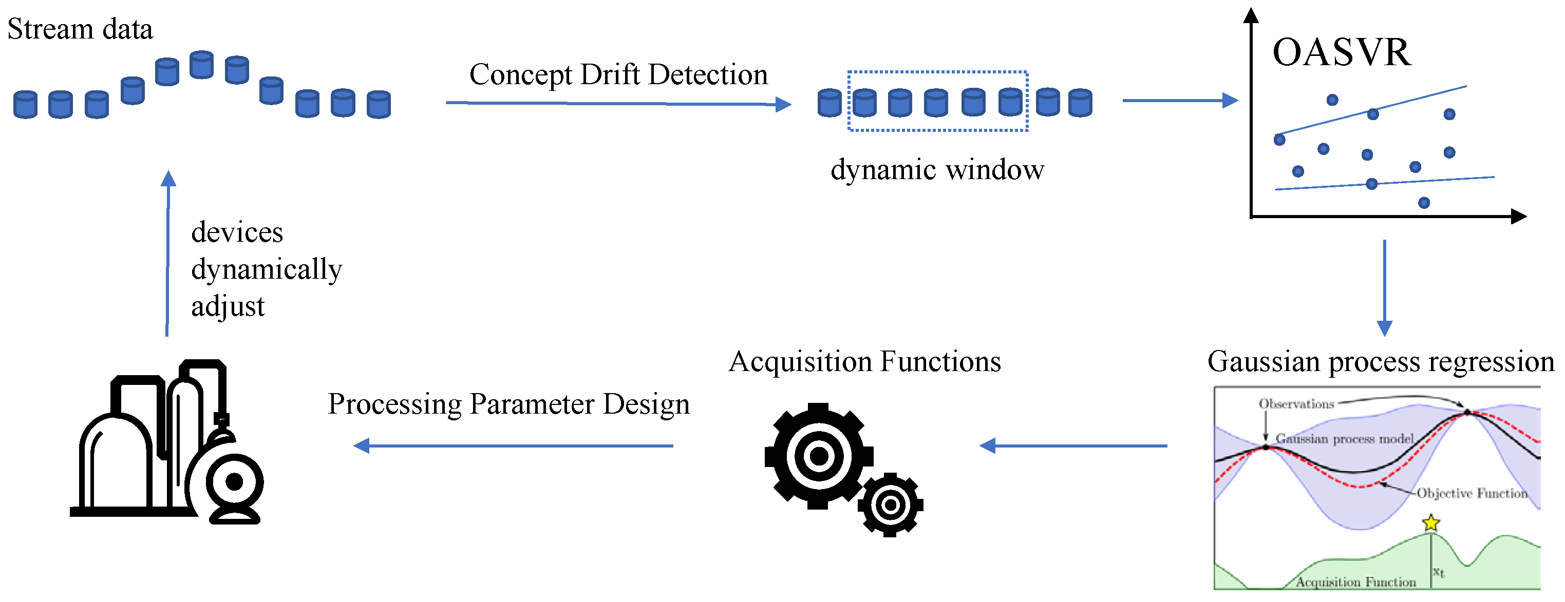
The proposed framework, which is shown in Figure 1, for the online processing parameters design in this paper follows the subsequent workflow: when the collected streaming data do not meet the pre-training quantity, a simple prediction is made. Once the quantity meets the pre-training requirement, concept drift detection is performed on the new streaming data. If concept drift is detected, this portion of data is discarded to prevent incorrect updates to the model. If no drift occurs, the online machine learning model parameters are updated to predict the next round of process performance. The streaming data without concept drift are used to update a Gaussian process regression model and Bayesian optimization is carried out using a Gaussian maximum upper confidence acquisition function with an adaptive learning rate. This process completes the reverse design and recommendation of process parameters. Factory equipment automatically adjusts according to the designed process parameters. Then, new streaming data are collected again for the next round of process parameter recommendations.
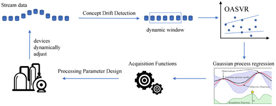
Figure 1.
Online processing parameters design framework. Apply concept drift detection on the streaming data collected from industrial equipment, eliminate data affected by drift and incorporate these refined data into the OASVR model for online learning. Utilize Bayesian optimization based on the predictions of model for processing parameter design. The industrial devices will automatically adjust according to the recommended process parameters to achieve enhanced manufacturing outcomes.
Notation: To make the notations easier to follow, we give a summary of the notations in the following list:
- ϵ
- is the insensitive loss function and is defined as for a predicted value and a true output Y;
- K
- is the kernel function;
- b
- is the bias;
- C
- is a regularization constant;
- αi
- is the weight of ;
- are slack variables correspond to the magnitude of this excess deviation for positive and negative deviations, respectively;
- *1i
- is the ith * variable in the upper function;
- *2i
- is the ith * variable in the lower function.
3.1. Online Accelerated Support Vector Regression
For a training set , constructing a linear regression equation on the feature space F, as shown in Equation (1).
where w is a vector in the F space, maps the input x to a vector in F and denotes the inner product in reproducing kernel Hilbert space (RKHS). Here, optimization techniques can be employed to obtain w and b for solving problems.
where is a regularization term that characterizes the complexity of the regression model. The optimization criterion is used to penalize those values of Y that differ from by more than .
Each of these two equations determines the upper and lower bounds. Meanwhile, to make the constraints independent of the training size, the objective function of Equation (3) is multiplied by the size of the training sample set. Therefore, the problem of seeking the upper bound function is transformed into solving the following primal problems (QPPs):
where is denoted as . Its corresponding pairwise problem is shown in Equation (6).
where Q is a positive definite matrix . The lower bound function can be obtained by the same modification.
Based on Equations (3) and (5), this algorithm solves a pair of quadratic programming problems (QPPs) instead of one QPP. This means that a data point only needs to satisfy the conditions of one of these functions. This indicates that there is only one set of constraints on all data points in OASVR. This strategy of solving two smaller-sized QPPs instead of one large QPP means that OASVR is simpler than classical SVR.
With these modifications, the classical AONSVR is transformed into OASVR, where two smaller-sized QPPs need to be solved. Furthermore, the estimated upper and lower bounds of a regression model by OASVR effectively encapsulate the data distribution’s properties. This can enhance the robustness of the model in many situations. After estimating the upper and lower bound functions, the final regression function can be expressed as Equation (7).
The process of incremental learning is to change the weight corresponding to the new sample in a finite number of discrete steps until it meets the KKT conditions, while ensuring that the existing samples in the training set continue to satisfy the KKT conditions at each step [17]. And, decremental learning is employed when an existing sample is removed from the training set. If a sample is in the remainder set, then it does not contribute to the SVR solution and removing it from the training set is trivial; no adjustments are needed. If, on the other hand, the sample has a nonzero weight, then the idea is to gradually reduce the value of the weight to zero while ensuring that all the other samples in the training set continue to satisfy the KKT conditions.
Although the above modifications will reduce the training time of the model, with the continuous increase in streaming data, the training time of the model will inevitably increase. In order to ensure that the model can meet the computation time requirements of different industrial scenarios, we add a dynamic window for the training data, and the dynamic window will be adjusted according to the model performance. At the beginning of training, the initial size of the dynamic window is set and the model will keep training until the window size is satisfied. After each online update of OASVR, we determine whether the RMSE of the model decreases; if the RMSE of the model decreases, the size of the dynamic window is increased by 1. If the RMSE of the model increases, we apply decremental learning to the first streaming data in the dynamic window. The maximum window size can also be set to ensure computational efficiency.
3.2. Concept Drift Detection
Concept drift detection refers to techniques and mechanisms that characterize and quantify concept drift by identifying change points or change intervals. Common concept drift detection methods are categorized into the following three types: model-error-rate-based methods, data-distribution-based methods and multiple-hypothesis-testing-based methods [11]. Among them, data-distribution-based methods use a distance function to quantify the difference between historical data distributions and new data. If the difference between the two proves to be statistically significant, it indicates that concept drift has occurred. Classical data-distribution-based detection algorithms include model-capability-based drift detection (SCD) [23], a least squares density difference change detection test (LSDD-CDT) [24] and others [12,25,26].
Liu et al. [27] proposed a data-distribution-based drift detection algorithm called equal intensity k-means space partitioning (EI-kMeans) for concept drift detection via histograms. Traditional data-distribution-based algorithms for detecting distribution-based drift seek to develop a novel test statistic to quantify the disparity between two distributions and craft a tailored hypothesis test to assess the significance of drift [28]. Conversely, EI-kMeans concentrates on the efficient transformation of multivariate samples into multinomial distributions, subsequently employing established hypothesis tests for concept drift detection. Utilizing Pearson’s chi-square test [29] as its hypothesis testing method, EI-kMeans enables the direct calculation of drift thresholds from the chi-square distribution, facilitating online implementation. In this paper, if the p-value, which is the result of the Pearson’s chi-square test, is greater than 0.05, the test data are considered to have experienced concept drift.
3.3. The Reverse Design of Processing Parameters Based on Bayesian Optimization
The adaptability of online machine learning allows models to quickly adjust to changing data distributions, providing more accurate predictions. Bayesian optimization [30] efficiently selects the most promising experimental configurations during experiments, thereby reducing costs and time. Combining the strengths of both, the reverse design of Bayesian optimization using high-precision online machine learning models that continually adapt to new data is highly beneficial for rapid iteration in industrial settings.
In Bayesian optimization, the choice of the acquisition function is crucial as it directly impacts the performance and efficiency of the Bayesian optimization algorithm. The primary role of the acquisition function is to help Bayesian optimization select the next point in the candidate point set for experimentation or evaluation, with the aim of maximizing the expected improvement in the objective function while striking a balance between exploring unknown regions and exploiting known optimal regions. Currently, an effective strategy [30] for achieving this balance is to encourage the selection of data points in unknown regions during the early stages of model iterations when there are limited observed data and the model has greater uncertainty. As the model undergoes multiple iterations, the focus shifts toward selecting points in regions where the optimal solution is likely to exist, given the increased amount of observed data and that the model has converged toward the optimal solution.
We select the maximum confidence upper bound function with an adaptive learning rate as the acquisition function, and its formula is as follows:
where t is the time step, denotes the mean, denotes the variance and is the weight, according to Srinivas et al. [28], who formulated a schedule for . For the weights of this framework, we adopt the following calculation method:
where is a constant from 0 to 1, a, b and r are constants greater than 0, d is the dimension of the optimization objective and t is the time step. In the maximum confidence upper bound function, the mean represents exploitation (knowledge of the model) and the variance represents exploration (selection of data in an unknown region). The adaptive learning rate decreases from large to small over time. The larger the weighting of variance, the greater the model uncertainty and the more likely it is to explore areas not observed by the model; conversely, the smaller the weighting of variance, the more the model focuses on stability and favors existing data. The adaptive learning rate can be weighed against the importance of the mean versus the uncertainty.
The reverse design process for process parameters is as follows: set the candidate range for process parameters and the objective function as the minimum difference between the predicted value and the target performance of material. Update the Gaussian process regression model based on the acquired streaming data. The Gaussian process regression model can predict the mean and variance of material performance based on the input process parameters. Use the acquisition function, Equation (8), to select the most likely candidate values in the candidate range of process parameters and input them into the objective function. Iterate until the maximum number of rounds, selecting the candidate point that best satisfies the objective function as the recommendation for the next round of process parameters.
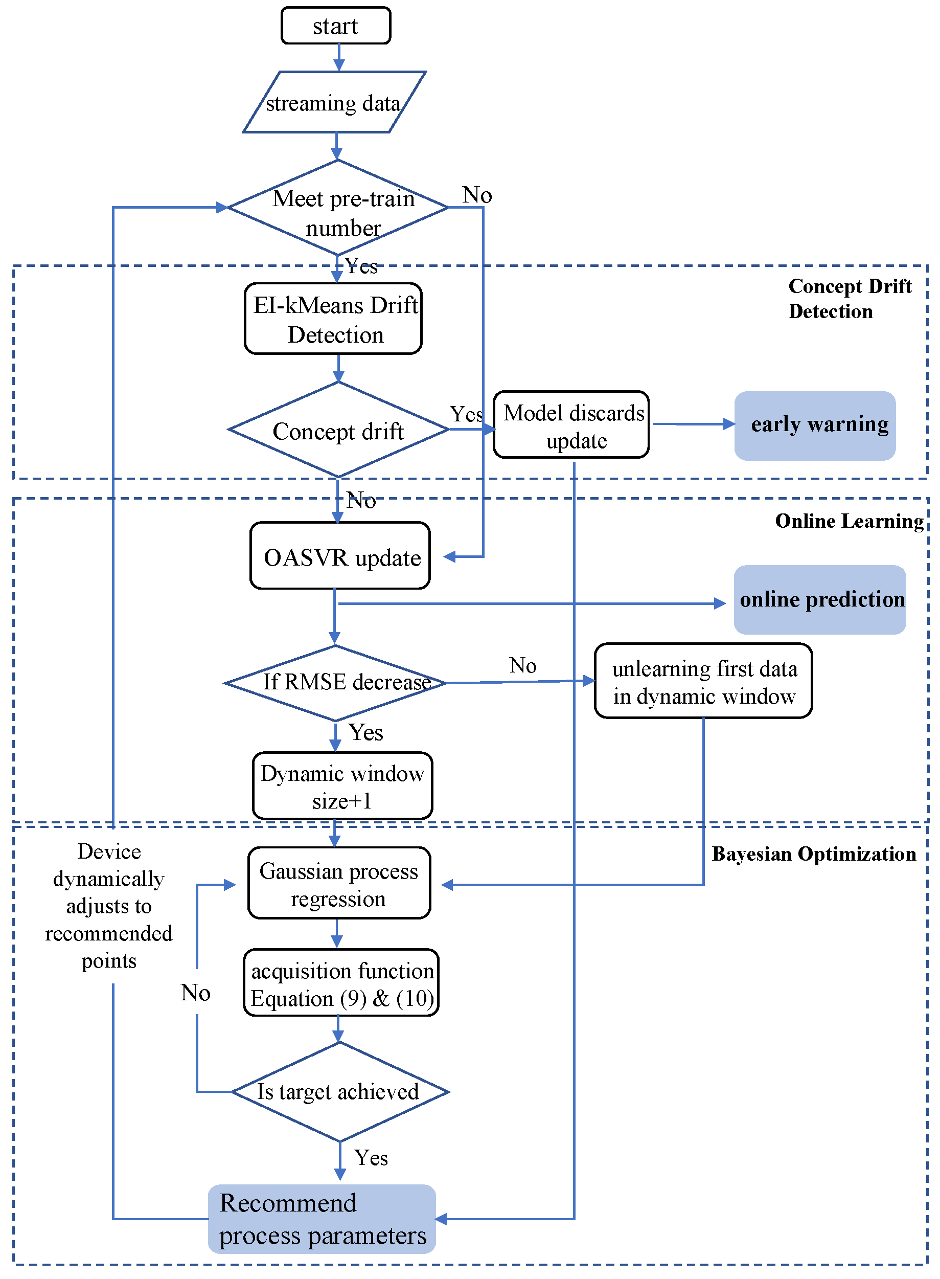
The overall algorithm execution flow for the online optimization and design of process parameters combining EI-kMeans concept drift detection, OASVR and adaptive learning rate Bayesian optimization is shown in Figure 2. Utilizing this framework allows for online data drift detection and warning in industrial scenarios and the online prediction of equipment processing performance, as well as the online optimization and recommendation of equipment process parameters.
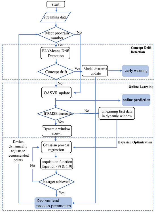
Figure 2.
The flowchart of OPPD framework, including three main parts: concept drift detection, online machine learning and Bayesian optimization.
4. Experimental Section and Results Analysis
Taking germanium single-crystal growth as an example, we apply the online accelerated support vector regression (OASVR) model. Through online model training, we predict the diameter of germanium single crystals and employ Bayesian optimization for the reverse design, recommending the pulling rate for the next moment in crystal growth to maintain the uniform radial growth of the single crystal.
4.1. Dataset
The production of photovoltaic-grade germanium single crystals using the Czochralski process [31] primarily includes seeding, necking, shoulder formation, shoulder rotation, radial growth and tailing. A seed crystal is positioned above the molten germanium ingot and under controlled temperature conditions, and it is immersed into the molten germanium to induce non-uniform nucleation. By designing an appropriate thermal field, both longitudinal and radial temperature distributions are effectively managed. During the radial growth stage, the seed crystal is rotated at a specific speed and pulled upward, allowing the newly solidified crystal to gradually grow into a single crystal. Of particular importance in crystal growth is the radial growth stage. We collected data from industrial equipment. To effectively build the model, we selected four datasets that represent relatively complete and valid data from the radial growth stage. Four datasets are denoted as K1 (1123 data points), K2 (400 data points), K3 (2015 data points) and K4 (1501 data points). Given that the primary parameters affecting germanium single-crystal growth are the crystal pulling rate (mm/h), crystal length (mm) and average liquid surface temperature (°C), these three parameters are chosen as the three-dimensional features for the model input. The objective of the experiment is to provide recommendations for the crystal growth pulling rate to maintain the uniform radial growth of the single crystal.
4.2. Experimental Setup
As a baseline comparison algorithm, this paper selects three other incremental learning algorithms, adaptive Hoeffding tree [32], SAM-kNN regressor [33] and adaptive random forest [34], for comparing the predictive and process parameter design performance of OASVR, as well as OASVR with regular SVR and AONSVR. Both tree-based models have high learning performance and low demands with respect to input preparation and hyperparameter tuning. And, the size of the sliding window for SAM-kNN can be continuously adapted during training.
The online model is trained incrementally with each incoming data point. At timestamp t, the model predicts the data at timestamp t based on the training data from timestamp 1 to . The performance of the model is evaluated by calculating the difference between the actual and predicted values.
We use RMSE and as evaluation metrics for the model. RMSE stands for root mean square error and is a commonly used metric in statistics and machine learning to measure the accuracy of predictions of the model. It quantifies the difference between predicted values and actual values, providing a single number that represents the overall error of the model. The equation for RMSE is as follows:
where n is the number of the dataset, is the actual value for the i-th data and is the predicted value. The lower the RMSE, the better the model performance.
The coefficient of determination, often denoted as , is a statistical measure that assesses the proportion of the variance in the dependent variable that can be explained by the independent variables in a regression model. The formula for is given as follows:
where is the mean of the actual values, and other variables have the same meanings as the variables in the RMSE formula. A higher value suggests that the model is better at explaining the variability in the dependent variable.
The experiment was conducted on a system running the Windows 10 operating system with an AMD Ryzen 7 4800H CPU with 16 GB of memory. Python version 3.8 and scikit-multiflow version 0.5.3 were employed.
4.3. Experiments and Result Analysis
The experiment utilized 60 pre-training samples with model evaluation based on . Comparative machine learning algorithms employed default hyperparameters, while AONSVR and OASVR utilized specific settings: C = 1, epsilon = 0.1, gamma = 0.1 and bias = 0.5. The initial size of the dynamic window was 200.
From the results in Table 1, it can be seen that the improved OASVR performs better on all datasets compared to AONSVR and regular SVR. For the four datasets, OASVR shows an average that is 2.2% higher than SVR and 4.15% higher than AONSVR, respectively. This indicates that the method of decomposing the original problem into two smaller quadratic programming problems is effective and demonstrates high robustness in such high-noise datasets. Among other incremental learning algorithms, OASVR performs best on all datasets. Adaptive Hoeffding tree and adaptive random forest are both tree-based ensemble learning regression algorithms, obtaining the final result through the votes of multiple decision trees. This approach may not perform well for small samples and low-dimensional datasets. The SVR series models, on the other hand, can effectively handle such types of data.

Table 1.
Comparison of prediction accuracy () between OASVR and other algorithms.
4.3.1. Comparative Experiments between OASVR, SVR and AONSVR
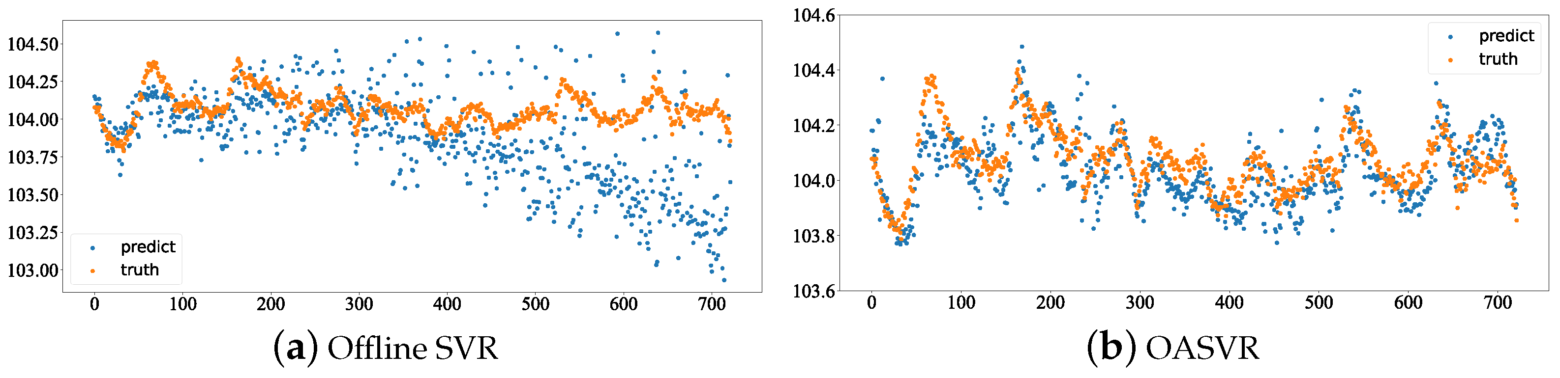
We compared OASVR with offline SVR, with the experiment set on the same dataset (K3 dataset). Initially, we pre-trained both models with 500 data points using the same hyperparameters. We then compared the prediction performance of OASVR and offline SVR, and the results are shown in the following Figure 3.
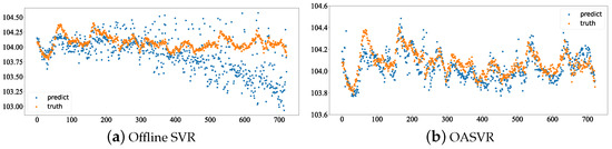
Figure 3.
Comparison of prediction results between offline SVR and OASVR.
OASVR has an RMSE of 0.126, while offline SVR has an RMSE of 0.36. It is evident that dynamic model updates can lead to better model prediction performance.
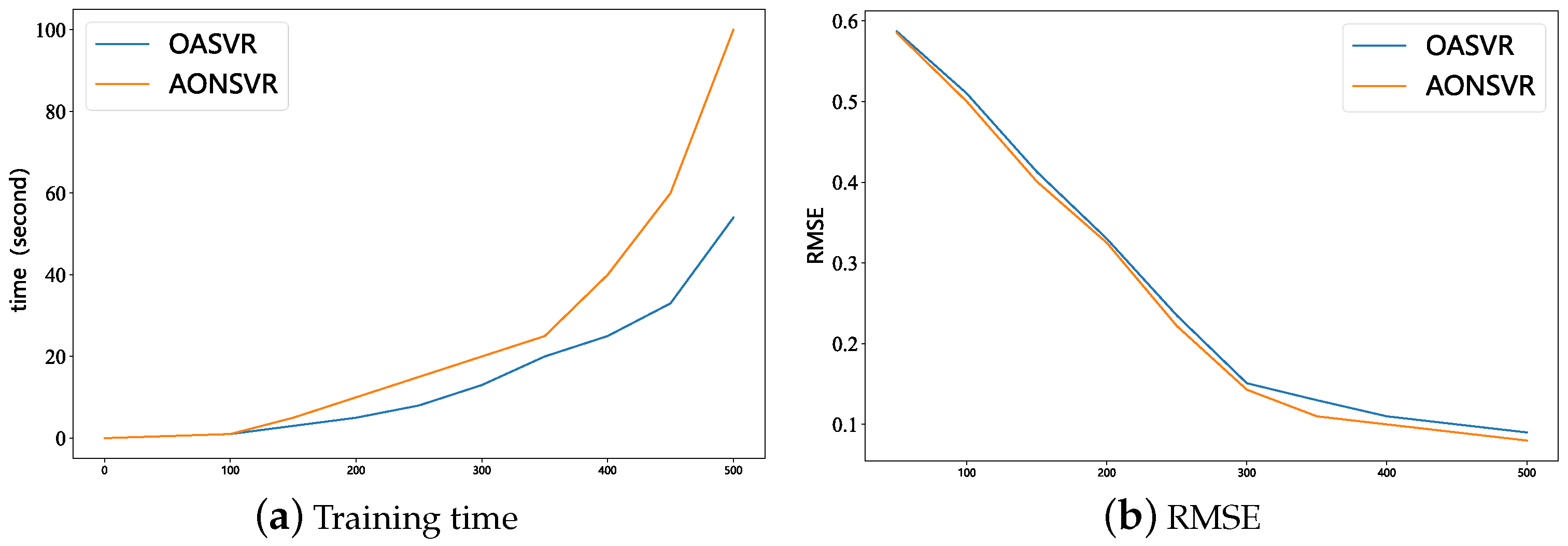
We conducted a comparative experiment on the performance of AONSVR and OASVR on the same dataset (K3 dataset), with the same hyperparameter set. We compared the training time and model accuracy of the two models, and the results are shown in Figure 4 below.
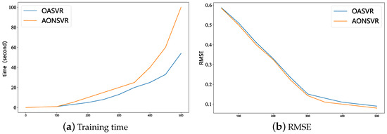
Figure 4.
Comparison of OASVR and AONSVR training time and prediction accuracy.
Figure 4a represents the training time of the model. From the graph, we can see that, with the same training samples, the training time of the model is reduced by half, while, comparing with Figure 4b, the prediction performance of the model is not significantly reduced. With a training data size of 500, the RMSE for OASVR is 0.09, while the RMSE for AONSVR is 0.07. This indicates that the OASVR algorithm has similar performance to AONSVR but is more efficient.
4.3.2. Visual Analysis of Different Online Machine Learning Models for Prediction
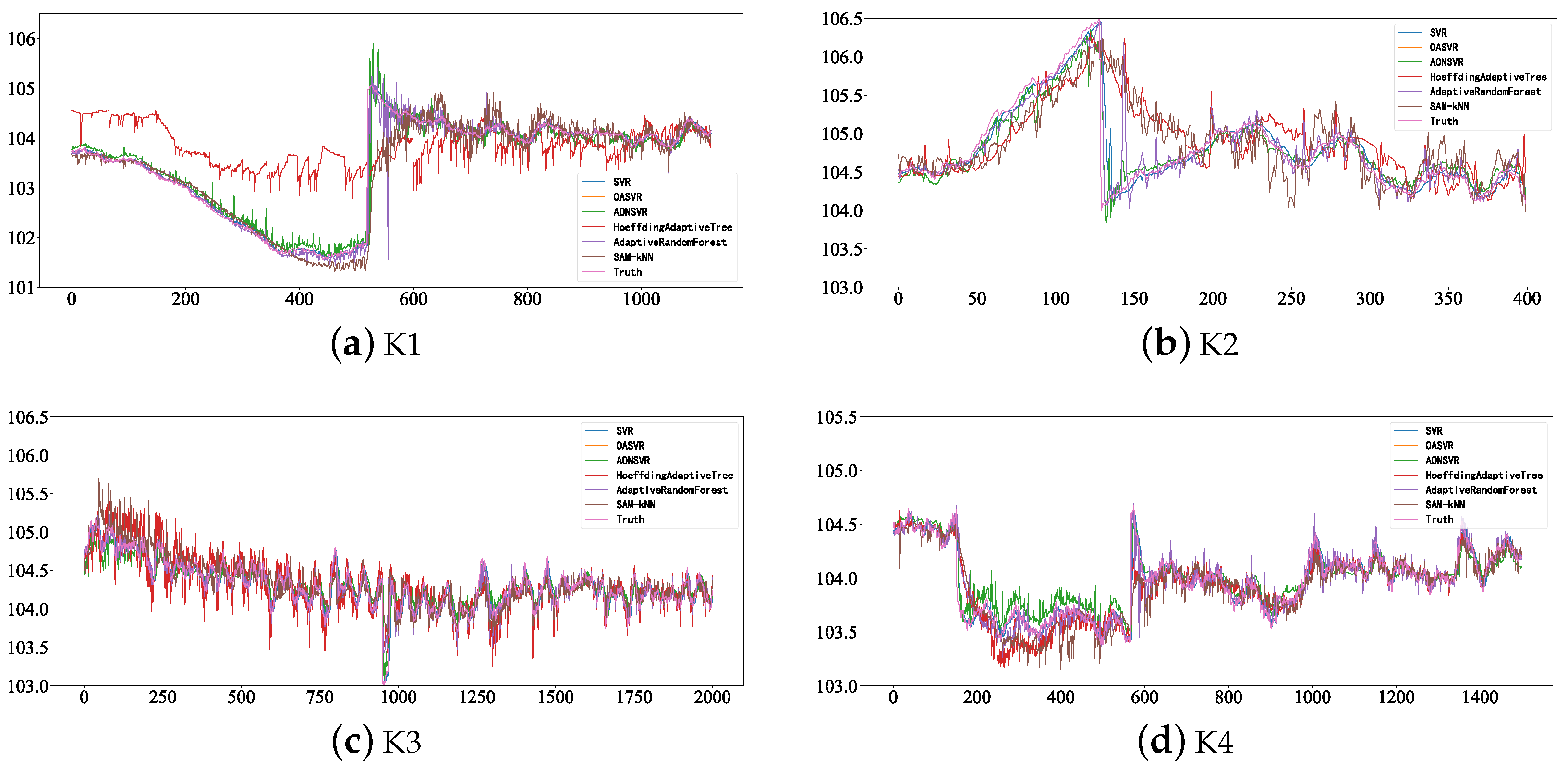
The predictive results illustrated in Figure 5 reveal that OASVR performs best on four datasets. There is concept drift to varying degrees in all four datasets, which shows that, where concept drift occurs, there will be significant fluctuations between the predicted values of the model and the actual values. These concept drift occurrences will affect the performance of the model. Therefore, for actual industrial scenarios, it is necessary to conduct concept drift detection on newly collected streaming data.
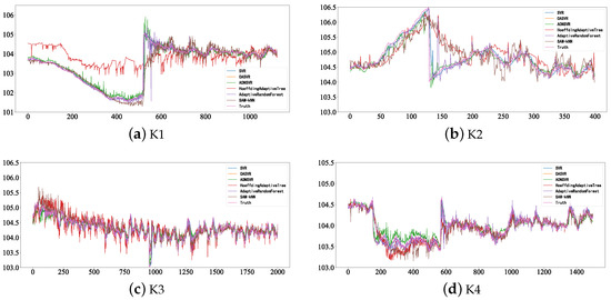
Figure 5.
Predictive results from five online machine learning models, SVR, OASVR, AONSVR, Hoeffding adaptive tree and adaptive random forest.
4.3.3. Dynamic Window Size and Computation
Figure 6 shows the size of the dynamic window and the corresponding time required to train each streaming data during the OASVR training process on different datasets. The training time for each streaming data is approximately 5 s, and the addition of the dynamic window effectively controls the training time as the size of dataset increases compared to the original model. Furthermore, it allows for the adjustment of appropriate window sizes in various industrial scenarios to meet diverse time constraints. According to Figure 6c, it can be observed that the window size reaches only up to 394 when the train number reaches 2000 due to the presence of a dynamic window mechanism. This significantly reduces computational load while still maintaining favorable model performance.
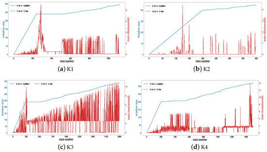
Figure 6.
Dynamic window size and corresponding training time for each streaming data during the OASVR training process on four different datasets: K1, K2, K3, K4.
4.4. Concept Drift Detection
The EI-kMeans method is chosen to perform concept drift detection for OASVR. The detection window size refers to the number of detection data points used for concept drift detection. In industrial scenarios, we aim to minimize the lag in concept drift detection. And, the Pearson’s chi-square test requires a minimum data count of 5 for detection. So, the window size is set to 10 and the number of clusters is set to 2.
When the number of new streaming data points reaches the detection window size, the Pearson’s chi-squared test is applied to the new data to detect concept drift. The test calculates a p-value and, if the p-value is greater than 0.05, it indicates that concept drift has occurred. For the detected drift data, they will be discarded and not used in the model training. The results with the inclusion of concept drift detection are shown in Table 2 below:
Table 2.
Before and after OASVR incorporates concept drift detection results.
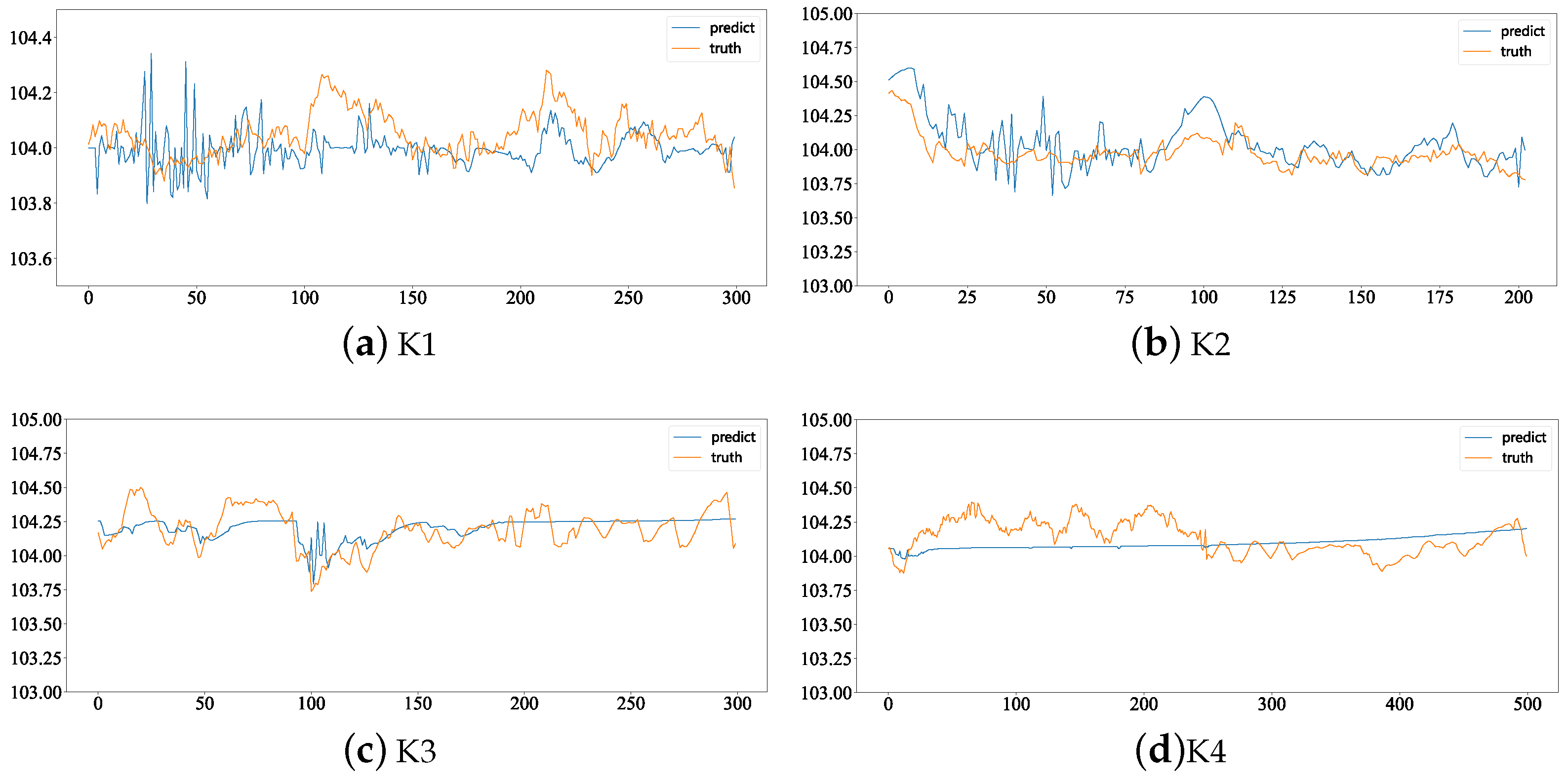
The predictive results after incorporating concept drift detection are shown in Figure 7. From Table 2, we can know that the average of OASVR-EIk is 1.85% higher than OASVR on four datasets. Figure 7 shows the predictive result of OASVR-EIk. While OASVR demonstrates some capability in handling noise, it still struggles with abrupt concept drift. OASVR-EIk does not online train the data detected by EI-kMeans as experiencing concept drift. This prevents OASVR from updating weights for erroneous data, allowing the model to fit a more reasonable data distribution and thus improving the overall performance.
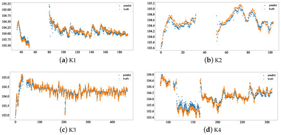
Figure 7.
Predictive results of OASVR-EIk on four different datasets: K1, K2, K3 and K4.
4.5. Process Parameter Design Based on Bayesian Optimization
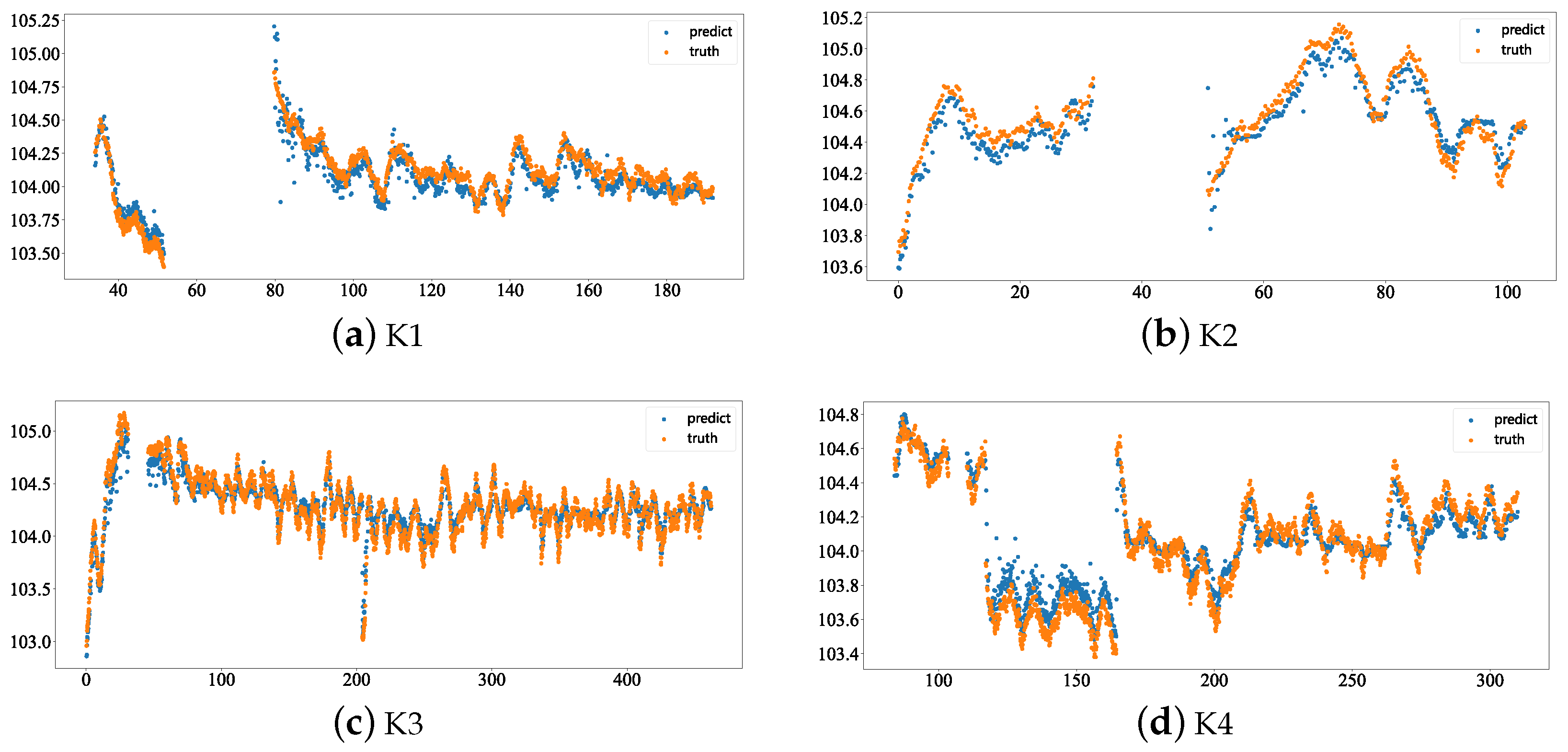
In this experiment, the model was applied to four germanium single-crystal datasets. Due to the inherent time delay associated with adjusting the average liquid level temperature, the optimized process parameter was the actual crystal growth rate. The hyperparameters for Bayesian optimization were set with a maximum of 20 iterations and the acquisition function used Equation (9). The target prediction value was set to 104 and the objective of Bayesian optimization was to make the predicted diameter value of model as close as possible to the target prediction value. Figure 8 shows the prediction results.
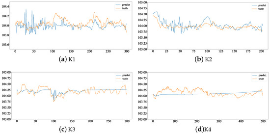
Figure 8.
Comparison between predictive results of recommended pulling rate and the real one on four different datasets: K1, K2, K3 and K4.
On the four datasets K1, K2, K3 and K4, the RMSE values are 0.21, 0.09, 0.13 and 0.05, with an average RMSE of 0.12. From Figure 8, it can be observed that the recommended points obtained through Bayesian optimization mostly remain within a range of ±0.5 from a diameter value of 104. Additionally, it is noticeable from the figure that the first half of the iterations for the recommended points show significant variations, while, in the later stages, they tend to approach the actual values. This suggests that the adaptive learning rate helps to balance exploration and exploitation effectively. Comparing the trends in actual values and predicted values, such as the section between 100 and 200 in the K1 chart and the section between 50 and 100 in the K3 chart, the actual diameter values start above 104. With the changes in recommended points, the actual values gradually decrease and approach 104, ultimately maintaining the actual diameter values within the allowable error range of the target diameter value.
5. Discussion
The OASVR model outperforms other online models across all datasets. The method used by OASVR to calculate upper and lower bounds separately shows higher robustness compared to AONSVR, especially performing better on datasets with concept drift. Adaptive Hoeffding tree and adaptive random forest struggle to effectively handle low-dimensional and small-sample datasets, which may be a contributing factor to their subpar performance. For the streaming data where concept drift is detected, the current drift adaptation method only discards these data. Changing the algorithm to adapt to concept drift to incrementally update the model will be one of our future works.
To enhance computational efficiency, we introduced a dynamic window, adjusting its size dynamically based on the performance of the model. This approach has effectively improved efficiency, yet some issues persist. In real industrial scenarios, the real-time requirement of the model is very high and only the algorithm has been improved; in the future, we will combine hardware and software acceleration, such as putting the matrix calculation into the FPGA computing unit for calculation, to further improve the computational speed of the model.
6. Conclusions
In this paper, we propose an online process parameter prediction and design framework that integrates online machine learning, concept drift detection and Bayesian optimization to enhance computational efficiency and adaptability in dynamic industrial settings.
We refine the AONSVR algorithm, proposing the online adaptive support vector regression (OASVR). The OASVR doubles computational efficiency with equivalent data sizes to AONSVR. Our framework employs online machine learning models for real-time process prediction and reverse engineering. The online machine learning model can dynamically update weights and Bayesian optimization is used to dynamically design process parameters. An acquisition function with an adaptive learning rate is used in Bayesian optimization to balance exploration and exploitation. We incorporate concept drift detection to ensure accurate model updates and a dynamic window size to optimize computational efficiency. These strategies enhance the capability of the framework to cater to the varied requirements of diverse industrial environments. We applied this framework to the germanium single-crystal dataset and achieved excellent results.
Author Contributions
Y.Y.: data curation, software, implementation, investigation, formal analysis, visualization, writing—original draft. Q.Q.: conceptualization, methodology, funding acquisition, project administration, supervision, writing—review and editing. All authors have read and agreed to the published version of the manuscript.
Funding
This work was sponsored by the National Key Research and Development Program of China (No. 2023YFB4606200), Key Program of Science and Technology of Yunnan Province (No. 202302AB080020) and Key Project of Shanghai Zhangjiang National Independent Innovation Demonstration Zone (No. ZJ2021-ZD-006).
Data Availability Statement
The source code that supports the findings of this study are available at https://github.com/Yyb0b/OPPR (accessed on 1 March 2024).
Acknowledgments
The authors gratefully appreciate the anonymous reviewers for their valuable comments.
Conflicts of Interest
The authors declare that they have no known competing financial interests or personal relationships that could have appeared to influence the work reported in this paper.
References
- Ghobakhloo, M. Industry 4.0, digitization, and opportunities for sustainability. J. Clean. Prod. 2020, 252, 119869. [Google Scholar] [CrossRef]
- Rai, R.; Tiwari, M.K.; Ivanov, D.; Dolgui, A. Machine learning in manufacturing and industry 4.0 applications. Int. J. Prod. Res. 2021, 59, 4773–4778. [Google Scholar] [CrossRef]
- Jordan, M.I.; Mitchell, T.M. Machine learning: Trends, perspectives, and prospects. Science 2015, 349, 255–260. [Google Scholar] [CrossRef] [PubMed]
- Fontenla-Romero, Ó.; Guijarro-Berdiñas, B.; Martinez-Rego, D.; Pérez-Sánchez, B.; Peteiro-Barral, D. Online machine learning. In Efficiency and Scalability Methods for Computational Intellect; IGI Global: Hershey, PA, USA, 2013; pp. 27–54. [Google Scholar]
- Ikonomovska, E.; Loshkovska, S.; Gjorgjevikj, D. A survey of Stream Data Mining. 2007. Available online: https://repository.ukim.mk/handle/20.500.12188/23843 (accessed on 7 March 2024).
- He, H.; Chen, S.; Li, K.; Xu, X. Incremental learning from stream data. IEEE Trans. Neural Netw. 2011, 22, 1901–1914. [Google Scholar] [PubMed]
- Ma, J.; Theiler, J.; Perkins, S. Accurate on-line support vector regression. Neural Comput. 2003, 15, 2683–2703. [Google Scholar] [CrossRef] [PubMed]
- Gu, B.; Sheng, V.S.; Wang, Z.; Ho, D.; Osman, S.; Li, S. Incremental learning for ν-support vector regression. Neural Netw. 2015, 67, 140–150. [Google Scholar] [CrossRef] [PubMed]
- Yu, H.; Lu, J.; Zhang, G. An incremental dual nu-support vector regression algorithm. In Proceedings of the Advances in Knowledge Discovery and Data Mining: 22nd Pacific-Asia Conference, PAKDD 2018, Melbourne, VIC, Australia, 3–6 June 2018; Springer: Berlin/Heidelberg, Germany, 2018; pp. 522–533. [Google Scholar]
- Gu, B.; Wang, J.D.; Yu, Y.C.; Zheng, G.S.; Huang, Y.F.; Xu, T. Accurate on-line ν-support vector learning. Neural Netw. 2012, 27, 51–59. [Google Scholar] [CrossRef]
- Lu, J.; Liu, A.; Dong, F.; Gu, F.; Gama, J.; Zhang, G. Learning under concept drift: A review. IEEE Trans. Knowl. Data Eng. 2018, 31, 2346–2363. [Google Scholar] [CrossRef]
- Lu, N.; Zhang, G.; Lu, J. Concept drift detection via competence models. Artif. Intell. 2014, 209, 11–28. [Google Scholar] [CrossRef]
- Lakshminarayanan, B.; Roy, D.M.; Teh, Y.W. Mondrian forests: Efficient online random forests. Adv. Neural Inf. Process. Syst. 2014, 27, 3140–3148. [Google Scholar]
- Ikonomovska, E.; Gama, J.; Džeroski, S. Online tree-based ensembles and option trees for regression on evolving data streams. Neurocomputing 2015, 150, 458–470. [Google Scholar] [CrossRef]
- Yu, C.; Zhang, R.; Huang, Y.; Xiong, H. High-dimensional knn joins with incremental updates. Geoinformatica 2010, 14, 55–82. [Google Scholar] [CrossRef]
- Pham, D.T.; Dimov, S.S.; Nguyen, C. An incremental K-means algorithm. Proc. Inst. Mech. Eng. Part C J. Mech. Eng. Sci. 2004, 218, 783–795. [Google Scholar] [CrossRef]
- Yu, H.; Lu, J.; Zhang, G. An online robust support vector regression for data streams. IEEE Trans. Knowl. Data Eng. 2020, 34, 150–163. [Google Scholar] [CrossRef]
- Liu, J.; Zio, E. A SVR-based ensemble approach for drifting data streams with recurring patterns. Appl. Soft Comput. 2016, 47, 553–564. [Google Scholar] [CrossRef]
- Cauwenberghs, G.; Poggio, T. Incremental and decremental support vector machine learning. Adv. Neural Inf. Process. Syst. 2000, 13. [Google Scholar]
- Carvajal Soto, J.; Tavakolizadeh, F.; Gyulai, D. An online machine learning framework for early detection of product failures in an Industry 4.0 context. Int. J. Comput. Integr. Manuf. 2019, 32, 452–465. [Google Scholar] [CrossRef]
- Xie, Q.; Suvarna, M.; Li, J.; Zhu, X.; Cai, J.; Wang, X. Online prediction of mechanical properties of hot rolled steel plate using machine learning. Mater. Des. 2021, 197, 109201. [Google Scholar] [CrossRef]
- Malaca, P.; Rocha, L.F.; Gomes, D.; Silva, J.; Veiga, G. Online inspection system based on machine learning techniques: Real case study of fabric textures classification for the automotive industry. J. Intell. Manuf. 2019, 30, 351–361. [Google Scholar] [CrossRef]
- Song, X.; Wu, M.; Jermaine, C.; Ranka, S. Statistical change detection for multi-dimensional data. In Proceedings of the 13th ACM SIGKDD International Conference on Knowledge Discovery and Data Mining, San Jose, CA, USA, 12–15 August 2007; pp. 667–676. [Google Scholar]
- Bu, L.; Alippi, C.; Zhao, D. A pdf-free change detection test based on density difference estimation. IEEE Trans. Neural Netw. Learn. Syst. 2016, 29, 324–334. [Google Scholar] [CrossRef]
- Gu, F.; Zhang, G.; Lu, J.; Lin, C.T. Concept drift detection based on equal density estimation. In Proceedings of the 2016 International Joint Conference on Neural Networks (IJCNN), Vancouver, BC, Canada, 24–29 July 2016; pp. 24–30. [Google Scholar]
- Qahtan, A.A.; Alharbi, B.; Wang, S.; Zhang, X. A pca-based change detection framework for multidimensional data streams: Change detection in multidimensional data streams. In Proceedings of the 21th ACM SIGKDD International Conference on Knowledge Discovery and Data Mining, Sydney, NSW, Australia, 10–13 August 2015; pp. 935–944. [Google Scholar]
- Liu, A.; Lu, J.; Zhang, G. Concept drift detection via equal intensity k-means space partitioning. IEEE Trans. Cybern. 2020, 51, 3198–3211. [Google Scholar] [CrossRef] [PubMed]
- Srinivas, N.; Krause, A.; Kakade, S.M.; Seeger, M. Gaussian process optimization in the bandit setting: No regret and experimental design. arXiv 2009, arXiv:0912.3995. [Google Scholar]
- Sedgwick, P. Pearson’s correlation coefficient. BMJ 2012, 345, e4483. [Google Scholar] [CrossRef]
- Frazier, P.I. A tutorial on Bayesian optimization. arXiv 2018, arXiv:1807.02811. [Google Scholar]
- Wang, G.; Sun, Y.; Yang, G.; Xiang, W.; Guan, Y.; Mei, D.; Keller, C.; Chan, Y.D. Development of large size high-purity germanium crystal growth. J. Cryst. Growth 2012, 352, 27–30. [Google Scholar] [CrossRef]
- Bifet, A.; Gavalda, R. Adaptive learning from evolving data streams. In Proceedings of the Advances in Intelligent Data Analysis VIII: 8th International Symposium on Intelligent Data Analysis, IDA 2009, Lyon, France, 31 August–2 September 2009; Springer: Berlin/Heidelberg, Germany, 2009; pp. 249–260. [Google Scholar]
- Jakob, J.; Artelt, A.; Hasenjäger, M.; Hammer, B. SAM-kNN regressor for online learning in water distribution networks. In Proceedings of the International Conference on Artificial Neural Networks, Bristol, UK, 6–9 September 2022; Springer: Berlin/Heidelberg, Germany, 2022; pp. 752–762. [Google Scholar]
- Gomes, H.M.; Bifet, A.; Read, J.; Barddal, J.P.; Enembreck, F.; Pfharinger, B.; Holmes, G.; Abdessalem, T. Adaptive random forests for evolving data stream classification. Mach. Learn. 2017, 106, 1469–1495. [Google Scholar] [CrossRef]

Disclaimer/Publisher’s Note: The statements, opinions and data contained in all publications are solely those of the individual author(s) and contributor(s) and not of MDPI and/or the editor(s). MDPI and/or the editor(s) disclaim responsibility for any injury to people or property resulting from any ideas, methods, instructions or products referred to in the content. |
© 2024 by the authors. Licensee MDPI, Basel, Switzerland. This article is an open access article distributed under the terms and conditions of the Creative Commons Attribution (CC BY) license (https://creativecommons.org/licenses/by/4.0/).