1. Introduction
The demand for wireless bandwidth with Quality of Service (QoS) and ubiquitous network connectivity is continuously increasing due to the explosive growth in data traffic caused by a new generation of innovative high data rate services and applications accessed from a wide variety of wireless devices [
1,
2].
To address this issue, wireless backhaul networks that connect Macro Base Stations (MBSs) and Small Cells (SCs) are becoming popular as they use multiple-input multiple-output (Massive MIMO) and millimeter-wave (mmWave) transmission technologies [
3,
4,
5,
6] that use multiple antennas to provide significant improvements in wireless data transmission rates, link efficiency, network reliability, and energy efficiency [
7,
8]. They achieve high spectral efficiency by serving many users simultaneously and enabling the placement of a dense number of SCs within the MBSs coverage area [
9]. These SCs consist of low-power radio transmitter nodes that can handle the traffic of fixed and low-mobility users, which results in improved Quality of Service (QoS) in terms of throughput and outage as the distance between the access points and users is relatively short [
10,
11].
Although current wireless backhaul networks utilizing Massive MIMO and mmWave technologies show great potential in meeting the demands of current and future mobile Internet users, they require innovative network topology-control mechanisms that surpass those implemented in conventional cellular networks such as LTE or LTE-Advanced [
12]. This is essential for establishing a robust network backbone that fosters scalability and energy efficiency.
Topology control (TC) mechanisms aim to adapt the topology of a network to optimize performance metrics such as energy consumption while maintaining connectivity requirements throughout the network [
13,
14]. TC schemes were initially designed for Wireless Sensor Networks (WSNs), Mobile Ad Hoc Networks (MANETs), and Wireless Mesh Networks (WMNs) to improve overall performance [
15,
16,
17]. In wireless backhaul networks, the topology is adjustable by modifying parameters such as transmission power and antenna radiation patterns [
18,
19].
TC is generally challenging because there are several objective metrics to optimize, some potentially conflicting (e.g., energy consumption and robustness). To make the problem more tractable, we propose focusing the search for feasible topologies on
expander-like graphs, which are sparse graphs with “good” connectivity properties [
20,
21]. More specifically, we propose to search for topologies with high Laplacian Spectral Gap (LSG), which measures the strength of network connectivity and entanglement [
22].
The proposed algorithm takes advantage of the directional beamforming capability of Massive MIMO systems to activate a set of feasible non-interfering communication links, which allows the efficient incorporation of a significant number of SCs within the MBS coverage, increasing the spatial reuse of bandwidth and increasing spectral efficiency.
To the best of our knowledge, SGTC is the first topology control algorithm that effectively employs the information provided by the LSG to optimize the network topology by simultaneously minimizing the number of links and network diameter while maximizing the network entropy and the number of edge-disjoint paths connecting any two stations in the backhaul network. All these topological properties are desirable for backhaul networks because sparse topologies are energy-efficient, the network diameter impacts the upper bound of the end-to-end delay, the network entropy is related to the network’s ability to distribute data traffic evenly across the network and promotes seamless traffic offloading from the MBSs to the SCs, and a higher number of edge-disjoint paths leads to better throughput and robustness.
The rest of the paper is organized as follows.
Section 2 presents and discusses related work on massive MIMO systems, Small Cells, topology control, and expander graphs in the context of our work.
Section 3.1 presents a set of definitions and assumptions that are used in the rest of the paper.
Section 3.3 presents the problem formulation.
Section 4 and
Section 4.3 present the details of the proposed topological control scheme.
Section 5 presents the results of a series of experiments characterizing the impact of the LSG of the topology on the overall network performance. Lastly, we present our concluding remarks in
Section 6.
2. Related Work
In the past, topology control mechanisms have been studied mainly in Wireless Mesh Networks, Wireless Mobile Ad Hoc Networks, and Wireless Sensor Networks. The main objective of this type of mechanism is to modify the network topology to induce connectivity properties and improve the overall network performance [
23,
24].
Recently, topology-control mechanisms have also become relevant in wireless backhaul networks because they can help improve efficiency, promote traffic offloading from the core network, and avoid bottlenecks in the backhaul network. For instance, in [
25], the authors propose planning schemes for microwave-based wireless backhaul networks based on tree topologies that jointly optimize multiple performance metrics, such as traffic hops (delay), long links, link crosses, small angles, and the sum of the link distances. In [
26], the authors propose an iterative heuristic algorithm that constructs topologies that maximize the total backhaul flow in wireless multi-hop backhaul networks composed of SCs and networked flying platform (NFP) hubs. In [
27], the authors show that if the topologies for Ultra-High-Dense Networks (UDN) combine MBSs and a dense tier of SCs, they can accomplish objectives of 5G networks such as meeting traffic demand while providing seamless coverage, high data rate for low-mobility users and spatial reuse. In [
10], a comprehensive survey about the architecture, performance metrics, and guidelines of 5G networks is presented. The authors show that accommodating Massive MIMO with Small Cells improves performance metrics such as energy efficiency, coverage, capacity, resource efficiency, and spectral efficiency.
In the context of topology control schemes, some works have proposed inducing expander-like topologies in networks [
28,
29]. The rationale behind these works is that
expander graphs are sparse graphs with strong connectivity properties [
20], and therefore, networks with expander-like topologies will tend to be robust even if they do not have a large number of links. In [
30], the authors investigate the relationship between the properties of expander topologies implemented by wireless networks (called Wireless Expanders ) and the performance of such wireless networks in terms of enabling efficient broadcast solutions. In [
31,
32], the authors model dynamic peer-to-peer (P2P) networks using expander graphs in which the spectral gap property is preserved under node insertions and deletions. In [
33], the authors show that communication networks with expander-like topologies tend to be flexible and easy to reconfigure and optimize.
Simulated annealing (SA) has been successfully used to solve complex problems in wireless networks. For example, in [
34], the authors use SA for wireless backhaul planning to maximize system performance regarding network throughput and delay while reducing infrastructure utilization. Similarly, in [
35], the authors propose an SA-based algorithm to solve a power consumption problem. The idea is to use SA to minimize the total power consumed by MBSs and SCs serving access and wireless backhaul links. Other works on the use of SA to optimize the performance of wireless networks are [
36,
37,
38]. All these works show the effectiveness of simulated annealing as an optimization technique in the context of wireless networks.
This literature review shows that, unlike our proposal that uses the LSG to find expander-like topologies that simultaneously optimize the network’s energy cost, robustness, diameter, and entropy, previous topology control algorithms for backhaul networks either restrict their search to three-based topologies [
25], or do not consider multiple objective functions [
26,
27,
28,
29,
30,
31,
32]. Although SA has been used in the past for wireless backhaul planning [
35], our algorithm is the first to incorporate the information provided by the LSG to find network topologies with low energy costs and strong connectivity properties.
3. System Model and Problem Formulation
In this section, we introduce the notation used in the paper and provide a detailed description of the system model. We also present the problem formulation for finding a network topology that minimizes the number of links and the network’s diameter while maximizing the network’s entropy and robustness.
3.1. System Model
We use a graph to model the topology of a wireless backhaul network composed of sets of Macro Base Stations (MBSs) M, Small Cells (SCs) S, and bidirectional wireless communication links between them, where is the set of all the stations. The position of the stations in the plane is determined by a function that assigns x and y coordinates to them. We use to denote the one-hop neighborhood of u.
We assume that the SCs have a coverage range of distance units, whereas the MBSs have a coverage range of distance units. From the values of the coverage ranges, we have the following two definitions.
Definition 1. A communication link between stations is feasible if when or when either u or v is in M; where is the Euclidean distance.
Definition 2. A network topology is feasible if every link is feasible.
We further assume that:
All the stations are static; namely, they have fixed positions.
All the MBs have the same capabilities and coverage range. They are implemented by a Massive MIMO system with antenna elements.
All the SCs have the same capabilities and coverage range. They are equipped with antenna elements capable of supporting multiple parallel data streams.
MBSs and SCs can support all the possible links with the other MBs and SCs placed in their corresponding coverage area. More specifically, for an MBS , the inequality holds. Similarly, for a SC , the inequality also holds.
The energy cost of establishing a link from station u to station v is proportional to .
All the SCs have relay functionality; namely, they can communicate with any of their one-hop neighbors.
For a given network topology , we use the following performance metrics:
Network Diameter (): Defined as the longest shortest path between any two stations in G. Networks with a small diameter tend to induce lower delays and reduce the energy used to transport a packet from sources to destinations.
Network Robustness (): Defined as the cardinality of the global minimum cut-set, which is equivalent to the minimum number of edge-disjoint paths connecting any two stations in the network. Networks with high robustness are more tolerant to link breaks due to interference or channel effects. This metric indicates the minimum number of edges that need to be removed to partition the network.
Network Cost (
): Defined as the sum of the length of the edges in the graph (see Equation (
1)). This metric is related to the power used by the network to establish and maintain all the communication links.
Network Entropy (
): Defined as the entropy (see Equation (
2)) over the probability mass function (see Equation (
3)) of using a particular link
as part of the shortest path connecting an arbitrary source-destination pair. Network entropy measures the amount of information about how data traffic will be distributed across a particular network by a specific shortest-path routing protocol. High values of network entropy indicate that a given shortest-path routing protocol will tend to distribute data traffic evenly across the network. On the other hand, low values of network entropy indicate that this shortest-path routing protocol will tend to concentrate data traffic on a subset of the links (those with a high probability of being part of the shortest path). Similar to the betweenness centrality [
39],
(see Equation (
2)) provides information about the influence of an edge over the data flows in a network. In this context, network entropy can also be considered a measure of the ability of the network topology to distribute the traffic load evenly among all the active links and, hence, among all the stations (MBSs and SCs) that compose the network.
In Equation (
3),
is a function that counts the shortest paths that include link
e and
is a normalization constant. Algorithm 1 shows the pseudocode to compute the value of function
f for a given
. The call to
(see line 4) returns a shortest path connecting two stations using a given shortest path algorithm. We assume that the implementation of the shortest path algorithm breaks ties arbitrarily but consistently and, hence, that it always computes the same shortest path for a given source-destination pair.
| Algorithm 1 f(e) |
- Input
A network , an edge . Output The value of .
- 1:
- 2:
- 3:
for alldo - 4:
- 5:
if then - 6:
- 7:
end if - 8:
end for - 9:
return ;
|
3.2. Laplacian Spectral Gap
Let
be the adjacency matrix of a network
where
if there is an edge from station
i to station
j and
otherwise. Let
be the degree matrix
of
G which is a diagonal matrix with
if
and,
otherwise. From these two matrices, we can compute the Laplacian Matrix of the network
as
[
40]. Since a simple graph can represent the networks under consideration (links are bidirectional),
is a symmetric, positive semidefinite matrix that is also known as the combinatorial Laplacian matrix or Kirchoff matrix. For this type of network,
has a set of
real eigenvalues
,
,..,
where the second smallest eigenvalue (
) is called the
Laplacian Spectral Gap, LSG [
40] of the network
G. A large value of LSG implies a higher expansion, meaning that the network is generally well connected [
20]. This type of graph is associated with
Expander Graphs, a family of sparse graphs with strong connectivity properties [
41].
3.3. Problem Formulation
From the previous concepts and definitions, we formally state the problem of computing optimized wireless backhaul network topologies composed of MBs and SCs as follows.
Problem Formulation 1. Given a set of wireless backhaul entities located at positions in the plane designated by function l, and radio ranges for SCs and for MBSs, find a set of feasible communication links, according to Definition 1, such that the Laplacian Spectral Gap of is maximized.
As we have already mentioned, the objective of maximizing the Laplacian Spectral Gap is to jointly optimize:
the Network Diameter of ;
the Network Robustness of ;
the Network Cost of and;
the Network Entropy
of
as defined in
Section 3.1.
In this first formulation, the location of all stations is part of the input and is specified a priori by the function l.
Another interesting network design problem is to find suitable locations for the Macro Base Stations, i.e., to find a function that assigns a location in the plane to the MBSs such that the network performance is optimized. In this case, only the number of MBSs, not their locations, is part of the input.
Problem Formulation 2. Given a set of SCs S located at positions in the plane designated by the function , a number m of MBSs, and radio range for SCs and for MBSs; find a function that assigns a location in the plane to the MBSs and a set of feasible communication links such that the Laplacian Spectral Gap of is maximized.
Table 1 summarizes the notation used throughout the paper.
4. SGTC: The Spectral Gap-Based Topology Control Algorithm
This section introduces the proposed spectral gap-based topology control (SGTC) algorithm for wireless backhaul networks. The SGTC algorithm employs the information provided by the LSG to optimize the network topology with respect to the four performance metrics defined in
Section 3.3. SGTC takes as input the set of network entities
(generically referred to as stations), an initial set
of links, functions
and
that map stations to positions in the plane, radio ranges for MBSs and SCs, and the value of
which determines the maximum number of iterations.
The SGTC algorithm employs the simulated annealing (SA) meta-heuristic technique to explore the feasible solution space, seeking network topologies that yield a high LSG (). As we describe in more detail in the following paragraphs, the annealing process implements a random walk over the feasible solution space where a new candidate solution is accepted with a probability proportional to its LSG value and the current temperature of the annealing process. Initially, the temperature is set to a high value to promote a broad search of the solution space, and on each iteration, it is reduced to direct the random walk towards strictly better solutions.
After the annealing process is completed, SGTC calculates the Pareto front of the best feasible network topologies that were visited during the process. This calculation is based on three criteria: minimizing the network diameter and maximizing network robustness and entropy. SGTC returns the Pareto efficient solution with the lowest energy cost as its output.
4.1. The Feasible Solution Space
To implement the local search, we define the 1-feasible neighborhood of a network topology as the set composed of feasible network topologies such that can be obtained from E by adding or removing a single feasible link according to Definition 1. This way, the solution space can be organized as a graph with a vertex for each feasible network topology, and two vertices of this graph are adjacent if their corresponding network topologies differ in a single link.
As shown in the pseudocode of Algorithm 2, SGTC starts the simulated annealing process from an initial network topology
that is provided as an input parameter. The algorithm uses function
isFeasible() (see Line 2 of Algorithms 2 and 3) to check whether the initial topology is valid. If
is not feasible, the annealing process will start from an empty graph. From this point, SGTC performs a walk over the solution space graph by randomly selecting as the new candidate solution a network topology
from the 1-feasible neighborhood of the current solution
. By using function
getFeasibleRandomNeighbor() (see Line 8 of Algorithms 2 and 4) to select candidate solutions, the search performed by SGTC is restricted to feasible network topologies.
| Algorithm 2 SGTC Algorithm |
- Input:
A set of stations , an initial set of links , a function l that determines the stations’ position in the plane, radio ranges and , the initial temperature , and number of iterations - Output:
- 1:
; - 2:
if then - 3:
- 4:
else - 5:
- 6:
end if - 7:
for to do - 8:
- 9:
- 10:
- 11:
- 12:
if then - 13:
, , ; - 14:
else with probability - 15:
, - 16:
end if - 17:
- 18:
end for - 19:
- 20:
return
|
We decided to constrain the search to the feasible solution space because if an unfeasible link that increases the LSG is added to the network, the annealing process would be highly unlikely to remove it in future iterations to obtain a feasible topology. In such a scenario, from the point an unfeasible link is added to a solution, it will likely remain unfeasible until the end of the annealing process.
| Algorithm 3 is Feasible |
- Input:
A network topology , a function l that determines the stations’ position in the plane, and radio ranges and - Output:
True if the topology is feasible according to Definition 1, false otherwise.
- 1:
for all
do - 2:
if then - 3:
if then - 4:
return false - 5:
end if - 6:
else - 7:
if then - 8:
return false - 9:
end if - 10:
end if - 11:
end for - 12:
return true
|
| Algorithm 4 obtain Feasible Random Neighbor |
- Input:
A network topology , a function l that determines the stations’ position in the plane, and radio ranges and - Output:
A network topology or G if
- 1:
- 2:
for iterations do - 3:
- 4:
if then - 5:
return - 6:
else - 7:
if then - 8:
if then - 9:
return - 10:
end if - 11:
else - 12:
if then - 13:
return - 14:
end if - 15:
end if - 16:
end if - 17:
end for - 18:
return
G
|
4.2. The Annealing Process
Following the simulated annealing strategy, on each iteration of SGTC, a candidate solution is accepted as the new current solution with probability one if has a larger value of than that of the current solution , namely if (Line 12). It also accepts a candidate solution following the Metropolis criterion, with probability , if (Line 14). The control parameter , used in Line 11 of Algorithm 2 to compute the probability , takes the role of the temperature in the annealing process and is reduced at each iteration (see Line 17) to gradually force the search towards strictly better solutions.
SGTC stores in the feasible network topologies visited during the annealing process. Then, it uses ParetoFront() (see Line 19 of Algorithm 2) to determine the Pareto front composed of the solutions in that minimize the network diameter and maximize the network robustness and entropy.
Lastly, SGTC returns the network in of minimum energy cost (see Line 20 of Algorithm 2) as the output of the algorithm.
4.3. SGTC with Optimized MBS Placement
To address Problem Formulation 2, where the network designer can determine the location of the MBSs, we propose to find a set of locations that minimizes the maximum distance between any SC and its closest MBS. More formally, let be the distance between an SC and the set M of MBSs. We propose to find a function that assigns locations to the MBSs that minimize M’s covering radius , which equals .
This latter formulation corresponds to the vertex k-center problem (for
), a well-known NP-hard problem originally proposed by Hakimi in 1964 [
42]. Since the vertex k-center problem cannot be solved in polynomial time within an approximation factor of
[
43], unless P = NP, we propose using the Critical Dominating Set algorithm that has shown good performance in practice [
44,
45].
Once we have determined optimized locations for the MBSs, we can use the SGTC algorithm to look for a topology with a large Laplacian Spectral Gap.
4.4. Computational Complexity
The following theorem establishes the temporal complexity of the SGTC algorithm.
Theorem 1. The temporal complexity of the SGTC algorithm (Algorithm 2) is .
Proof of Theorem 1. The main loop of Algorithm 2 (lines 7–18) iterates times and contains calls to isFeasible() (Algorithm 3), getFeasibleRandomNeighbor() (Algorithm 4), and LSG() to compute the LSG of a network .
The complexity of Algorithm 3 is because it checks whether all the are feasible, and the maximum number of edges in a graph is in . Similarly, the complexity of Algorithm 4 is because, in the worst case, it performs iterations to identify a feasible link that will be either added or removed from E. Computing the LSG of a graph is dominated by the cost of determining its eigenvalues, which is because the Laplacian Matrices are symmetric. Therefore, the total complexity of the main loop is .
The complexity of computing the Pareto front of
N data points and three objective functions is
when we use Kung’s algorithm [
46]. So, if we select
we obtain
.
Therefore, the overall complexity of the SGTC algorithm is which is the same as . □
5. Experimental Results
In this section, we present the results of a series of experiments that characterize the ability of the SGTC algorithm to find network topologies that optimize the performance metrics presented in
Section 3.3, namely, that minimize the network diameter
, maximize the network robustness
, minimize the network cost
, and maximize the network entropy
.
For a given network topology
, and function
and
that assign the positions of the nodes in the plane, we compute its robustness
as the cardinality of the global minimum cut-set. To this end, we execute an instance of the Ford–Fulkerson algorithm [
47] over the
pairs of nodes. To compute the network entropy, we run Dijkstra’s algorithm [
48] for every pair of nodes and count the number of times (denoted by
) that a given
belongs to one of these shortest paths. Then, we use Equation (
3) to compute the probability of using a particular edge
e in the shortest path and compute
according to Equation (
2). The network diameter is easily obtained from the lengths of the shortest paths of all the pairs of nodes, and the network cost is computed according to Equation (
1).
For the experiments presented in this section, we generate problem instances by assuming an uncorrelated position of the network entities (stations) within a normalized squared region of
. Specifically, we compute each station’s
x and
y coordinates by sampling the continuous uniform distribution with bounds
, which assumes an uncorrelated position of the nodes [
49,
50].
As shown in
Table 2, we vary the total number of stations
from 100 to 200, the normalized radio range of the MBSs from 0.3 to 0.5, and the normalized radio range of the SCs from 0.15 to 0.2. The number of MBSs equals
to have scenarios where approximately
of the stations are MBSs. We further assume that all the stations have enough antennas to establish all the links determined by the SGTC algorithm.
The results presented in all the figures include the output of the proposed algorithm when using the following initial network topologies.
Disconnected: . The initial network has no links.
Feasible fully connected: is . The initial network contains all the feasible links.
Voronoi topology [
51]:
is
is
. The initial network contains all the feasible links connecting MBSs among themselves, and the SCs are connected to their closest MBSs if the corresponding link is feasible.
In all the experiments, the maximum number of iterations of the SGTC algorithm equals 10,000, and the initial temperature of the simulated annealing process equals 1.0. Each experiment is run for 20 independent seeds.
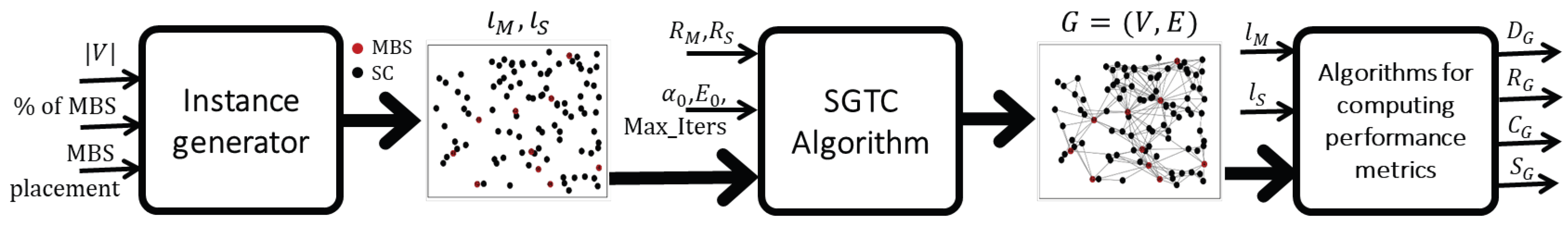
The experimental workflow composed of the instance generator, the SGTC algorithm, and a set of algorithms that compute the performance metrics is illustrated in
Figure 1. The instance generator algorithm takes the number of stations
, the percentage of MBSs, and the type of MBS placement (random or k-center) as input parameters. It returns functions
and
that determine the locations of MBSs and SCs, respectively.
Next, the SGTC algorithm uses the functions , , the initial set of links , and the values of the radio ranges and as input parameters to compute the resulting topology of the backhaul network. The initial temperature and the number of iterations are the hyper-parameters of SGTC.
Lastly, a set of algorithms compute the diameter , robustness , cost , and entropy of network G.
5.1. Performance as a Function of the LSG
Figure 2,
Figure 3,
Figure 4 and
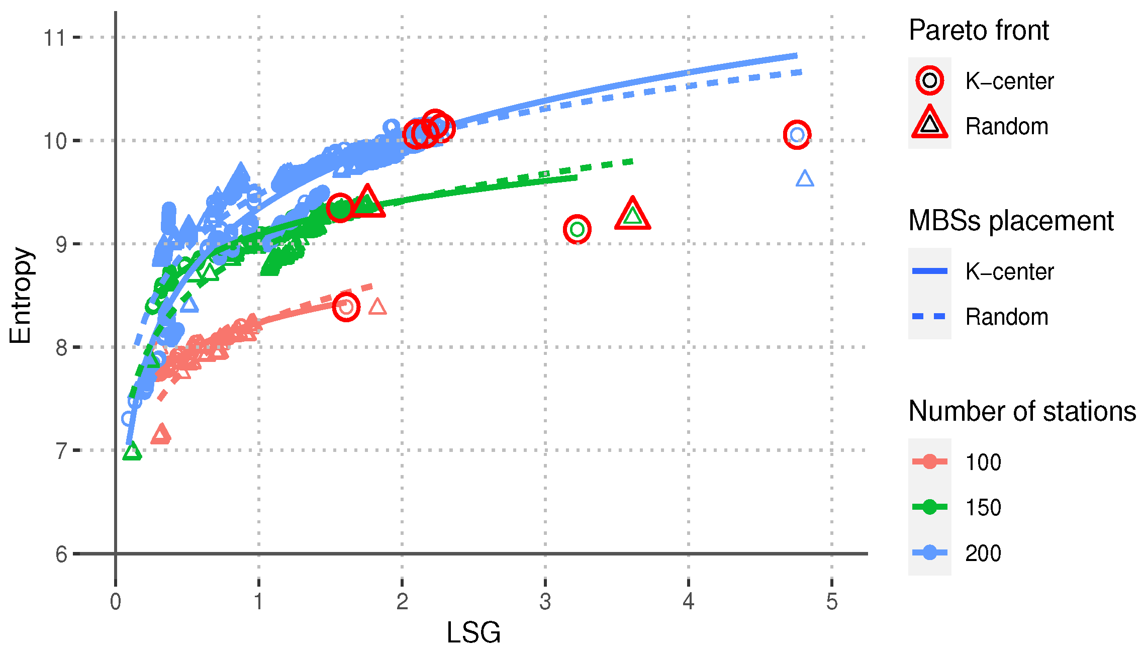
Figure 5 illustrate the behavior of the four performance metrics as a function of the value of the LSG. In the figures, each data point corresponds to a network topology found by SGTC during the annealing process, and the solid lines represent curves fitting the data points computed using logarithmic regression. The data points that belong to the Pareto front of the solutions that minimize the network diameter and maximize the network robustness and entropy are highlighted in black. For these results, we set the value of the normalized radio ranges
and
to 0.5 and 0.2, respectively. For the sake of clearness, the figures only present a representative sample of all the results; however, the tendencies shown in the figures hold across all our experiments.
From
Figure 2, we can observe that for all the values of the network size and the two types of MBS placement, the value of the network entropy
increases as the value of the LSG increases. This result indicates that networks with larger LSG distribute the shortest paths connecting the stations evenly among all the data links. This is important because this type of topology will promote the even distribution of the data traffic among the whole network, thus offloading traffic from the MBSs to the SCs and reducing the probability of contention hot spots.
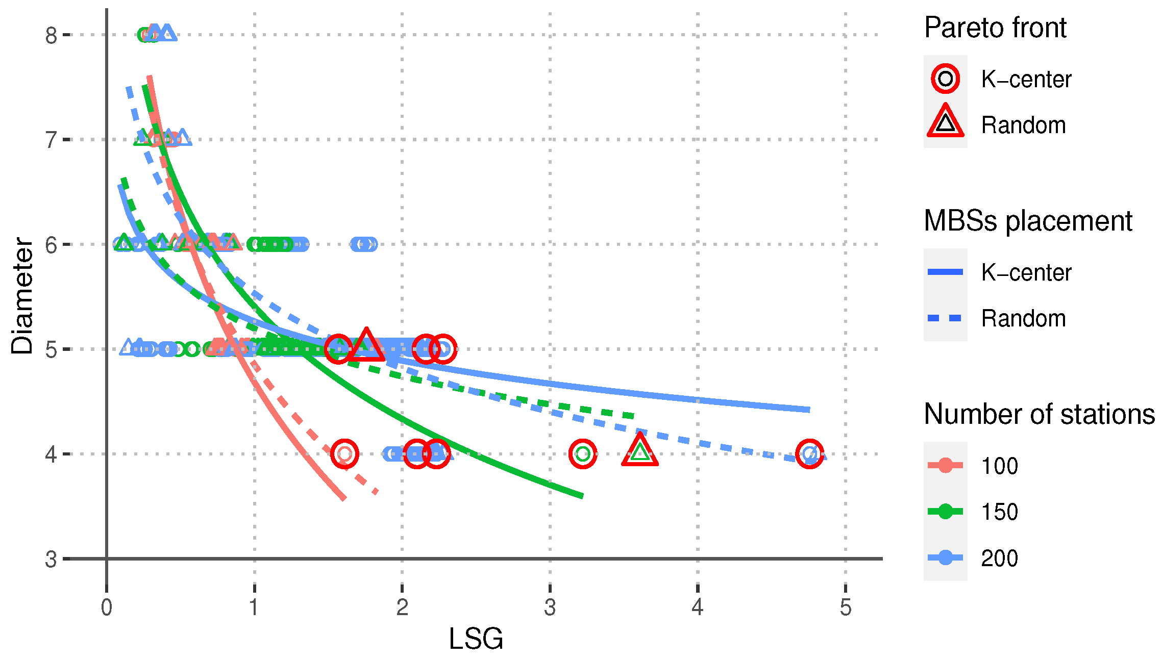
From
Figure 3, we can observe that, in general, the value of the network diameter
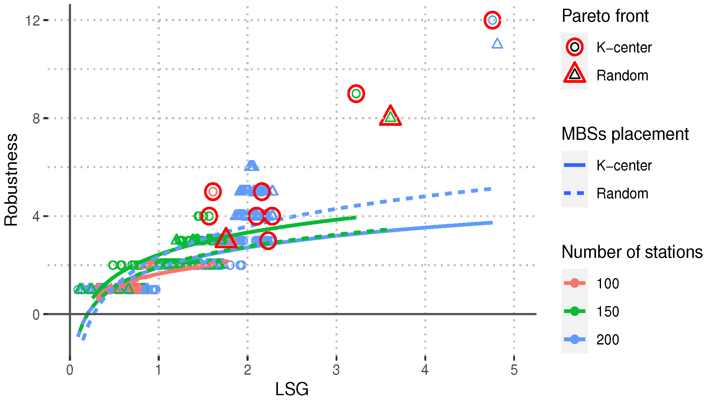
decreases as the value of the LSG increases, which indicates that the network gets better connected in terms of the length of the network’s largest shortest path. This positively impacts the upper bounds of the end-to-end delay and the energy needed to support an end-to-end data flow. Similarly,
Figure 4 shows that the network robustness
, measured as the cardinality of the network’s global minimum cut-set, increases as the LSG increases. This result indicates that networks with a larger value of LSG tend to be more robust to link breaks.
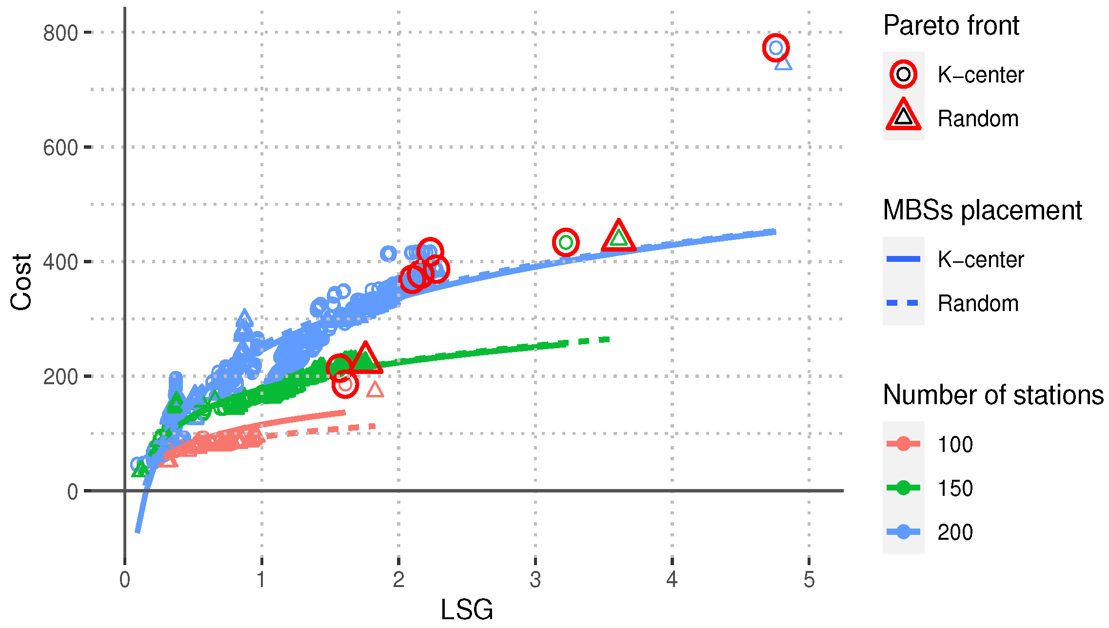
Lastly,
Figure 4 shows that the network cost
also increases as the LSG increases; however, for the case of networks of size 100 and 150, the rate at which the cost increases is reduced as the value of the LSG becomes larger. We can observe a similar trend for the networks of size 200 but with some exceptions for values of LSG larger than four. It is important to point out that SGTC avoids selecting these high-cost networks by selecting the Pareto efficient solution of minimum cost.
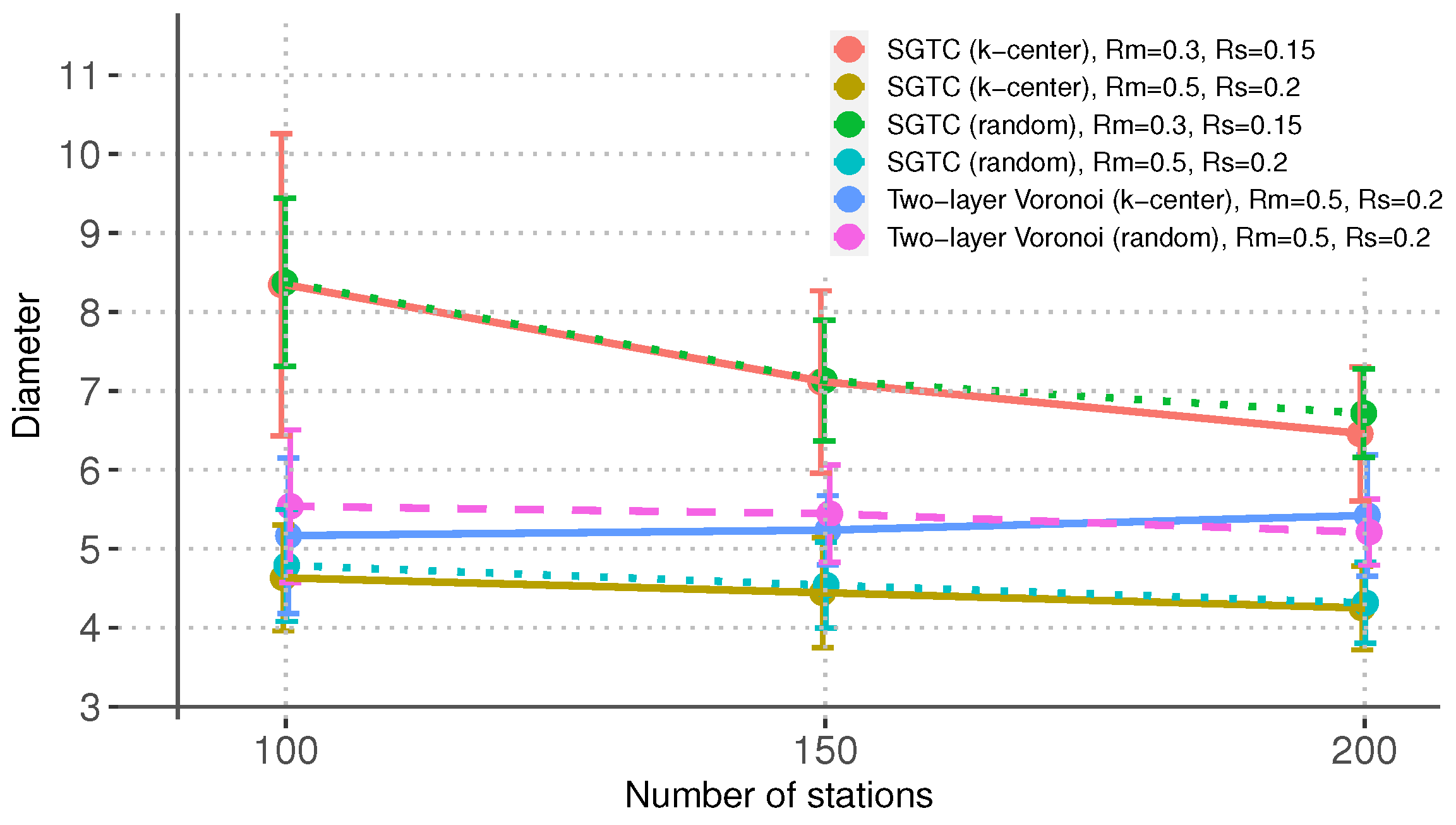
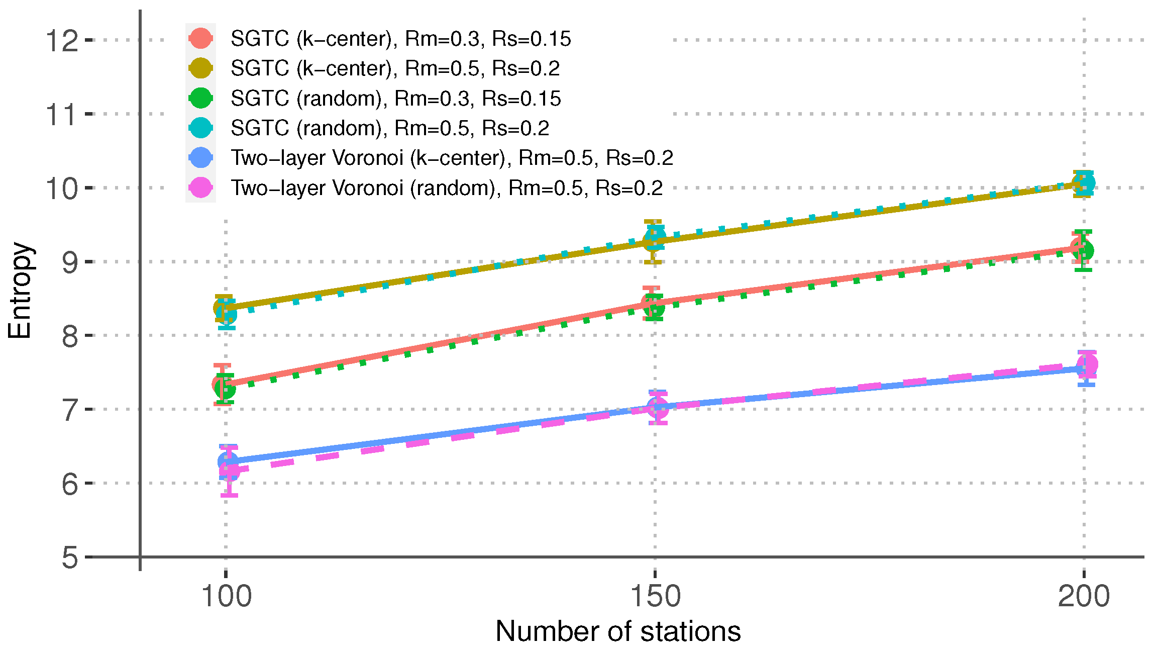
5.2. Performance Evaluation
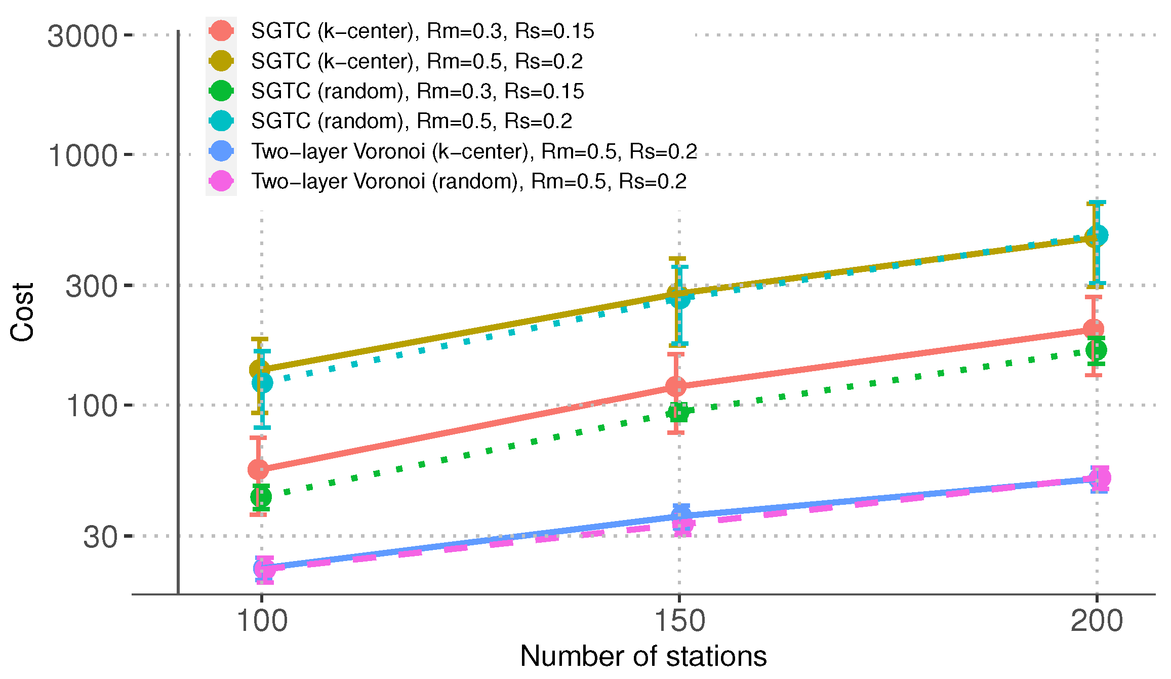
Figure 6,
Figure 7,
Figure 8 and
Figure 9 show the performance attained by SGTC when increasing the network size from 100 to 200 stations; MSBs are placed either at random or by solving the related k-center problem to minimize their covering radius; and for values of the stations’ radio ranges
and
. In order to have a performance baseline, we include the results of a traditional Voronoi-based algorithm that adds to the network all the feasible links connecting two MBSs and the feasible links connecting every SC to its closest MBS. In the figures, each point corresponds to the average result computed over 20 independent experiments, and the error bars correspond to the standard deviation value. Missing points in the graphs indicate that the corresponding algorithms could not connect the network in at least one of the twenty independent experiments.
From
Figure 6, we can observe that SGTC outperforms the traditional Voronoi-based algorithm by consistently achieving a higher value of network entropy
. The figure also shows that the network entropy benefits from having higher values of radio ranges. The reason is that the number of feasible links increases as the radio range increases, which also increases the space of feasible topologies that SGTC can investigate. From the figure, we can also notice that the MBS placement has no noticeable effect on this metric. Lastly, this figure does not include results for the Voronoi-based algorithm when
and
because the algorithm did not produce connected networks.
Figure 7 shows the network diameter
attained by the algorithms under the different scenarios. Similar to the case of the network entropy, SGTC produces the networks with the smallest diameters when
and
, which indicates that the algorithm can take advantage of a large space of feasible topologies to find well-connected networks. For
and
, the Voronoi-based algorithm achieves smaller values of network diameters by predominantly using the sub-network consisting of links between MBSs. This, however, has the disadvantage of concentrating the traffic in the MBSs. As for the previous metric, this figure shows that the MBS placement has no noticeable effect on the network diameter.
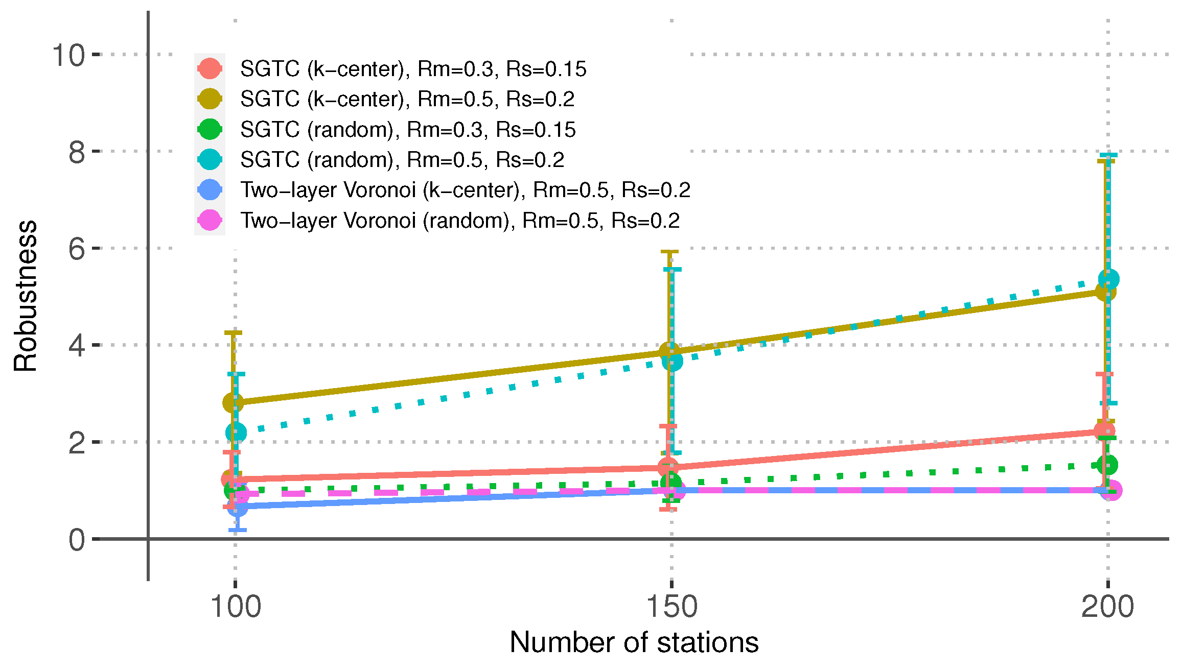
Figure 8 shows that the network robustness
follows a similar trend to that of the previous metrics. SGTC produces the most robust networks when the space of feasible topologies is larger, namely, when
, and there are many stations. However, unlike the case of the previous metrics, SGTC finds more robust networks for the case of
when the MBSs are placed using the k-center algorithm. The reason is that by reducing the covering radius of the MBS, the probability that all the SCs are within the radio range of an MBS is increased, which increases the probability of having more paths connecting the SCs to the rest of the network.
Lastly,
Figure 9 shows that the network cost
attained by the traditional Voronoi-based algorithm is smaller than that of SGTC. This result was expected because the Voronoi-based algorithm’s topologies include fewer links; the SCs are only connected to their closest MBS. As we saw in the previous metrics, this reduced cost comes at the expense of fragile, weakly connected networks that tend to concentrate traffic in the MBSs, increasing the probability of contention hot spots. This behavior becomes apparent when
,
because the links selected by the Voronoi-based algorithm are not enough to connect the network. On the other hand, even though the topologies generated by SGTC are more costly, we can observe that the rate at which this cost increases is similar to that of the Voronoi topologies. The reason is twofold. First, given that the cost of a network topology grows sublinearly with respect to the value of the LSG, the annealing process will not produce arbitrarily costly networks. Second, SGTC selects the Pareto efficient topology of minimum cost as its output.
6. Conclusions
We introduced the spectral gap-based topology control (SGTC) algorithm for wireless backhaul networks that uses simulated annealing guided by the value of the Laplacian Spectral Gap (LSG) to look for expander-like graphs, which are sparse graphs with strong connectivity properties such as small diameter, large value of the cardinality of its global minimum cut-set, and high shortest-path diversity. These are desirable properties for backhaul networks composed of Macro Base Stations and Small Cells because sparse topologies require less energy to establish and maintain their links, the diameter of a network impacts the upper bound of the end-to-end delay, the value of the cardinality of the global minimum cut-set determines the network robustness against link failures, and the shortest-path diversity promotes seamless traffic offloading from the MBSs to the Small Cells.
We presented network entropy as a measure of shortest-path diversity, which determines the amount of information about how data traffic is distributed across a particular network, where high values of network entropy indicate that data traffic will be evenly distributed across the network.
A series of experiments confirmed that the three connectivity metrics—diameter, robustness, and network entropy—improve as the value of the LSG increases, notably without requiring a significant increase in the number of links. This trend becomes more pronounced as the radio range of the stations increases because it increases the size of the space of feasible solutions. Our experimental results also showed that the topologies produced by SGTC are superior to those provided by a traditional Voronoi-based algorithm and that carefully placing the MBSs can improve the network robustness.
Future work includes conducting analytical and simulation-based analyses to determine the impact of expander-like topologies on the performance of upper-layer network functions, such as channel access and routing. We also plan to extend our algorithm to dynamically adapt the network’s topology to respond to the instantaneous traffic conditions. This is particularly important in the context of modern and future Internet applications where data traffic is bursty in nature, with large periods of low or no activity followed by sudden surges of high-intensity traffic.
Author Contributions
Conceptualization, S.J.G.-A., R.M.-M., S.A.P.-C. and M.E.R.-Á.; data curation, S.J.G.-A. and S.A.P.-C.; formal analysis, S.J.G.-A., R.M.-M., S.A.P.-C. and M.E.R.-Á.; investigation, S.J.G.-A. and R.M.-M.; methodology, S.J.G.-A., R.M.-M., S.A.P.-C. and M.E.R.-Á.; software, S.J.G.-A. and S.A.P.-C.; supervision, R.M.-M.; validation, S.J.G.-A., R.M.-M. and S.A.P.-C.; visualization, S.J.G.-A.; writing—original draft, S.J.G.-A., R.M.-M., S.A.P.-C. and M.E.R.-Á.; writing—review and editing, S.J.G.-A., R.M.-M., S.A.P.-C. and M.E.R.-Á. All authors have read and agreed to the published version of the manuscript.
Funding
This research was funded by the “Consejo Nacional de Humanidades Ciencias y Tecnologías” (CONAHCyT) of México and the “Instituto Politécnico Nacional” under grant SIP 20240950.
Data Availability Statement
Acknowledgments
We thank the technical support provided by the Data Science Lab of CITEDI-IPN.
Conflicts of Interest
Sergio Alejandro Pinacho-Castellanos is employee of corteza.ai company. The authors declare no conflicts of interest.
References
- Osseiran, A.; Boccardi, F.; Braun, V.; Kusume, K.; Marsch, P.; Maternia, M.; Queseth, O.; Schellmann, M.; Schotten, H.; Taoka, H.; et al. Scenarios for 5G Mobile and Wireless Communications: The Vision of the Metis Project. IEEE Commun. Mag. 2014, 52, 26–35. [Google Scholar] [CrossRef]
- Hirzallah, M.; Krunz, M.; Kecicioglu, B.; Hamzeh, B. 5G New Radio Unlicensed: Challenges and Evaluation. IEEE Trans. Cogn. Commun. Netw. 2021, 7, 689–701. [Google Scholar] [CrossRef]
- Ge, X.; Tu, S.; Mao, G.; Lau, V.K.; Pan, L. Cost Efficiency Optimization of 5G Wireless Backhaul Networks. IEEE Trans. Mob. Comput. 2019, 18, 2796–2810. [Google Scholar] [CrossRef]
- Alamu, O.; Iyaomolere, B.; Abdulrahman, A. An Overview of Massive MIMO Localization Techniques in Wireless Cellular Networks: Recent Advances and Outlook. Ad Hoc Netw. 2021, 111, 102353. [Google Scholar] [CrossRef]
- Ge, X.; Cheng, H.; Guizani, M.; Han, T. 5G Wireless Backhaul Networks: Challenges and Research Advances. IEEE Netw. 2014, 28, 6–11. [Google Scholar] [CrossRef]
- Zhai, B.; Tang, A.; Huang, C.; Han, C.; Wang, X. Antenna Subarray Management for Hybrid Beamforming in Millimeter-Wave Mesh Backhaul Networks. Nano Commun. Netw. 2019, 19, 92–101. [Google Scholar] [CrossRef]
- Khwandah, S.A.; Cosmas, J.P.; Lazaridis, P.I.; Zaharis, Z.D.; Chochliouros, I.P. Massive MIMO Systems for 5G Communications. Wirel. Pers. Commun. 2021, 120, 2101–2115. [Google Scholar] [CrossRef]
- Ali, M.Y.; Hossain, T.; Mowla, M.M. A Trade-off between Energy and Spectral Efficiency in Massive MIMO 5G System. In Proceedings of the 2019 3rd International Conference on Electrical, Computer & Telecommunication Engineering (ICECTE), Rajshahi, Bangladesh, 26–28 December 2019. [Google Scholar] [CrossRef]
- Rajoria, S.; Trivedi, A.; Godfrey, W.W. Energy Efficiency Optimization for Massive MIMO Backhaul Networks with Imperfect CSI and Full Duplex Small Cells. Wirel. Pers. Commun. 2021, 119, 691–712. [Google Scholar] [CrossRef]
- Rajoria, S.; Trivedi, A.; Godfrey, W.W. A Comprehensive Survey: Small Cell Meets Massive Mimo. Phys. Commun. 2018, 26, 40–49. [Google Scholar] [CrossRef]
- Yao, C.; Zhu, L.; Jia, Y.; Wang, L. Demand-Aware Traffic Cooperation for Self-Organizing Cognitive Small-Cell Networks. Int. J. Distrib. Sens. Netw. 2019, 15, 155014771881728. [Google Scholar] [CrossRef]
- Chataut, R.; Akl, R. Massive MIMO Systems for 5G and beyond Networks—Overview, Recent Trends, Challenges, and Future Research Direction. Sensors 2020, 20, 2753. [Google Scholar] [CrossRef]
- Kluge, R.; Stein, M.; Varró, G.; Schürr, A.; Hollick, M.; Mühlhäuser, M. A Systematic Approach to Constructing Families of Incremental Topology Control Algorithms Using Graph Transformation. Softw. Syst. Model. 2017, 18, 279–319. [Google Scholar] [CrossRef]
- Santi, P. Topology Control in Wireless Ad Hoc and Sensor Networks. ACM Comput. Surv. 2005, 37, 164–194. [Google Scholar] [CrossRef]
- Singla, P.; Munjal, A. Topology Control Algorithms for Wireless Sensor Networks: A Review. Wirel. Pers. Commun. 2020, 113, 2363–2385. [Google Scholar] [CrossRef]
- Shirali, N.; Jabbedari, S. Topology Control in the Mobile Ad Hoc Networks in Order to Intensify Energy Conservation. Appl. Math. Model. 2013, 37, 10107–10122. [Google Scholar] [CrossRef]
- Mudali, P.; Adigun, M.O. Context-Based Topology Control for Wireless Mesh Networks. Mob. Inf. Syst. 2016, 2016, 9696348. [Google Scholar] [CrossRef]
- Gui, J.; Zeng, Z. Joint Network Lifetime and Delay Optimization for Topology Control in Heterogeneous Wireless Multi-Hop Networks. Comput. Commun. 2015, 59, 24–36. [Google Scholar] [CrossRef]
- Liu, Y.; Hu, Q.; Blough, D.M. Joint Link-Level and Network-Level Reconfiguration for Urban Mmwave Wireless Backhaul Networks. Comput. Commun. 2020, 164, 215–228. [Google Scholar] [CrossRef]
- Hoory, S.; Linial, N.; Wigderson, A. Expander Graphs and Their Applications. Available online: https://www.ams.org/journal-getitem?pii=S0273-0979-06-01126-8 (accessed on 29 December 2023).
- Kleinberg, J.; Rubinfeld, R. Short Paths in Expander Graphs. In Proceedings of the 37th Conference on Foundations of Computer Science, Burlington, VT, USA, 14–16 October 1996. [Google Scholar] [CrossRef]
- Spielman, D.A. Spectral Graph Theory and its Applications. In Proceedings of the 48th Annual IEEE Symposium on Foundations of Computer Science (FOCS’07), Providence, RI, USA, 21–23 October 2007; pp. 29–38. [Google Scholar]
- Hu, S.; Li, G.; Huang, G. Dynamic Spatial-Correlation-Aware Topology Control of Wireless Sensor Networks Using Game Theory. IEEE Sens. J. 2021, 21, 7093–7102. [Google Scholar] [CrossRef]
- Wu, Y.; Hu, Y.; Su, Y.; Yu, N.; Feng, R. Topology Control for Minimizing Interference with Delay Constraints in an Ad Hoc Network. J. Parallel Distrib. Comput. 2018, 113, 63–76. [Google Scholar] [CrossRef]
- Li, Y.; Cai, A.; Qiao, G.; Shi, L.; Bose, S.K.; Shen, G. Multi-Objective Topology Planning for Microwave-Based Wireless Backhaul Networks. IEEE Access 2016, 4, 5742–5754. [Google Scholar] [CrossRef]
- Almohamad, A.; Hasna, M.O.; Khattab, T.; Haouari, M. An Efficient Algorithm for Dense Network Flow Maximization with Multihop Backhauling and Nfps. In Proceedings of the 2019 IEEE 90th Vehicular Technology Conference (VTC2019-Fall), Honolulu, HI, USA, 22–25 September 2019. [Google Scholar] [CrossRef]
- Gao, Z.; Dai, L.; Mi, D.; Wang, Z.; Imran, M.A.; Shakir, M.Z. MmWave Massive-MIMO-Based Wireless Backhaul for the 5G Ultra-Dense Network. IEEE Wirel. Commun. 2015, 22, 13–21. [Google Scholar] [CrossRef]
- Talak, R.; Karaman, S.; Modiano, E. Capacity and Delay Scaling for Broadcast Transmission in Highly Mobile Wireless Networks. In Proceedings of the 18th ACM International Symposium on Mobile Ad Hoc Networking and Computing, Chennai, India, 10–14 July 2017. [Google Scholar] [CrossRef]
- Pandey, P.K.; Badarla, V. Small-World Regular Networks for Communication. IEEE Trans. Circuits Syst. II Express Briefs 2020, 67, 1409–1413. [Google Scholar] [CrossRef]
- Attali, S.; Parter, M.; Peleg, D.; Solomon, S. Wireless Expanders. In Proceedings of the 30th on Symposium on Parallelism in Algorithms and Architectures, Vienna, Austria, 16–18 July 2018. [Google Scholar] [CrossRef]
- Pandurangan, G.; Robinson, P.; Trehan, A. Dex: Self-Healing Expanders. In Proceedings of the 2014 IEEE 28th International Parallel and Distributed Processing Symposium, Phoenix, AZ, USA, 19–23 May 2014. [Google Scholar] [CrossRef]
- Augustine, J.; Pandurangan, G.; Robinson, P.; Roche, S.; Upfal, E. Enabling Robust and Efficient Distributed Computation in Dynamic Peer-to-Peer Networks. In Proceedings of the 2015 IEEE 56th Annual Symposium on Foundations of Computer Science, Berkeley, CA, USA, 17–20 October 2015. [Google Scholar] [CrossRef]
- Avin, C.; Schmid, S. Toward Demand-Aware Networking. ACM SIGCOMM Comput. Commun. Rev. 2019, 48, 31–40. [Google Scholar] [CrossRef]
- Khaturia, M.; Appaiah, K.; Karandikar, A. On Efficient Wireless Backhaul Planning for the “Frugal 5G” Network. In Proceedings of the 2019 IEEE Wireless Communications and Networking Conference Workshop (WCNCW), Marrakech, Morocco, 15–18 April 2019. [Google Scholar] [CrossRef]
- Xu, X.; Saad, W.; Zhang, X.; Xiao, L.; Zhou, S. Dynamic on/off Control of Wireless Small Cells with Heterogeneous Backhauls. In Proceedings of the 2016 23rd International Conference on Telecommunications (ICT), Thessaloniki, Greece, 16–18 May 2016. [Google Scholar] [CrossRef]
- Leyva-Pupo, I.; Cervelló-Pastor, C. Efficient Solutions to the Placement and Chaining Problem of User Plane Functions in 5G Networks. J. Netw. Comput. Appl. 2022, 197, 103269. [Google Scholar] [CrossRef]
- Ganame, H.; Yingzhuang, L.; Hamrouni, A.; Ghazzai, H.; Chen, H. Evolutionary Algorithms for 5G Multi-Tier Radio Access Network Planning. IEEE Access 2021, 9, 30386–30403. [Google Scholar] [CrossRef]
- Chen, Y.-Y.; Chen, C. Simulated Annealing for Interface-Constrained Channel Assignment in Wireless Mesh Networks. Ad Hoc Netw. 2015, 29, 32–44. [Google Scholar] [CrossRef]
- Dolev, S.; Elovici, Y.; Puzis, R. Routing Betweenness Centrality. J. ACM 2010, 57, 1–27. [Google Scholar] [CrossRef]
- Preciado, V.M.; Jadbabaie, A.; Verghese, G.C. Structural Analysis of Laplacian Spectral Properties of Large-Scale Networks. IEEE Trans. Autom. Control 2013, 58, 2338–2343. [Google Scholar] [CrossRef]
- Karayel, E. Expander Graphs. Available online: https://www.isa-afp.org/entries/Expander_Graphs.html (accessed on 29 December 2023).
- Hakimi, S.L. Optimum Locations of Switching Centers and the Absolute Centers and Medians of a Graph. Oper. Res. 1964, 12, 450–459. [Google Scholar] [CrossRef]
- Hochbaum, D.S. Approximation Algorithms for NP-Hard Problems. ACM Sigact News 1997, 12, 40–52. [Google Scholar] [CrossRef]
- Garcia-Diaz, J.; Sanchez-Hernandez, J.; Menchaca-Mendez, R.; Menchaca-Mendez, R. When a Worse Approximation Factor Gives Better Performance: A 3-Approximation Algorithm for the Vertex K-Center Problem. J. Heuristics 2017, 23, 349–366. [Google Scholar] [CrossRef]
- Garcia-Diaz, J.; Menchaca-Mendez, R.; Menchaca-Mendez, R.; Pomares Hernandez, S.; Perez-Sansalvador, J.C.; Lakouari, N. Approximation Algorithms for the Vertex K-Center Problem: Survey and Experimental Evaluation. IEEE Access 2019, 7, 109228–109245. [Google Scholar] [CrossRef]
- Kung, H.T.; Luccio, F.; Preparata, F.P. On finding the maxima of a set of vectors. J. ACM 1975, 22, 469–476. [Google Scholar] [CrossRef]
- Ford, L.R.; Fulkerson, D.R. Maximal Flow through a Network. Can. J. Math. 1956, 8, 399–404. [Google Scholar] [CrossRef]
- Dijkstra, E.W. A Note on Two Problems in Connexion with Graphs. Numer. Math. 1959, 1, 269–271. [Google Scholar] [CrossRef]
- Yu, X.; Li, C.; Zhang, J.; Letaief, K.B. Analysis of Multi-Antenna Wireless Networks. In Stochastic Geometry Analysis of Multi-Antenna Wireless Networks; Springer: Singapore, 2019; pp. 85–125. [Google Scholar] [CrossRef]
- Miyoshi, N. Downlink Coverage Probability in Cellular Networks with Poisson—Poisson Cluster Deployed Base Stations. IEEE Wirel. Commun. Lett. 2019, 8, 5–8. [Google Scholar] [CrossRef]
- Okabe, A.; Boots, B.; Sugihara, K.; Chiu, S.N. Spatial Tessellations: Concepts and Applications of Voronoi Diagrams; John Wiley & Sons: New York, NY, USA, 2000. [Google Scholar]
| Disclaimer/Publisher’s Note: The statements, opinions and data contained in all publications are solely those of the individual author(s) and contributor(s) and not of MDPI and/or the editor(s). MDPI and/or the editor(s) disclaim responsibility for any injury to people or property resulting from any ideas, methods, instructions or products referred to in the content. |
© 2024 by the authors. Licensee MDPI, Basel, Switzerland. This article is an open access article distributed under the terms and conditions of the Creative Commons Attribution (CC BY) license (https://creativecommons.org/licenses/by/4.0/).


 ,
, 


