Acoustic TDOA Measurement and Accurate Indoor Positioning for Smartphone

Abstract

The global satellite navigation signal works well in open areas outdoors. However, due to its weakness, it is challenging to position continuously and reliably indoors. In this paper, we developed a hybrid system that combines radio signals and acoustic signals to achieve decimeter-level positioning indoors. Specifically, acoustic transmitters are synchronized with different codes. At the same time, our decoding scheme only requires a simple cross-correlation operation without time-frequency analysis. Secondly, acoustic signals will be reflected by glass, walls and other obstacles in the indoor environment. Time difference of arrival (TDOA) measurement accuracy is seriously affected. We developed a robust first path detection algorithm to obtain reliable TDOA measurement values. Finally, we combine the maximum likelihood (ML) algorithm with the proposed TDOA measurement method to obtain the location of the smartphone. We carried out static positioning experiments for smartphones in two scenes. The experimental results show that the average positioning error of the system is less than 0.5 m. Our system has the following advantages: (1) smartphone access. (2) an unlimited number of users. (3) easily deployed acoustic nodes. (4) decimeter-level positioning accuracy.

1. Introduction

Indoor positioning technology is the basis for emergency safety, crowd monitoring, precision marketing, entertainment and life, and human social needs [1]. At present, global navigation satellite systems (GNSS) can provide accurate positioning in open areas outdoors. However, mobile devices can hardly receive the GNSS signal because of the shelter of buildings. So it is unable to form effective indoor positioning by using the GNSS signal [2]. Common indoor positioning technologies include Wi-Fi [3] positioning technology, ultra-wide band (UWB) [4] positioning technology, optical positioning technology, and geomagnetic positioning technology [5,6]. These indoor positioning technologies have their own advantages and disadvantages, which are summarized as follows:

Wi-Fi positioning technology is mainly based on received signal strength (RSS), and fingerprint is established through signal strength characteristics [7]. This method is affected by the complex indoor topological environment. In recent years, Wi-Fi round trip time (RTT) has attracted the attention of scholars. In Wi-Fi RTT [8] positioning technology, the user can obtain distance information by calculating round trip time information between the mobile phone and the router. Mobile devices can be located through the trilateral positioning method. When using Wi-Fi RTT, mobile phone manufacturers need to provide the underlying information of Wi-Fi signals to users. However, Wi-Fi signals are vulnerable to indoor multipath [9]. Wi-Fi RTT positioning technology [10] has the following application limitations: the capacity of users is limited, and personal information security cannot be guaranteed. At present, only a few mobile phones support Wi-Fi RTT. The same frequency interference problem exists in Wi-Fi positioning technology [11]. A arrow band pulse signal is the signal source [12] in ultra-wide-band (UWB) positioning technology. The positioning process of the UWB positioning technology is as follows: (1) estimating the arrival time of the signal. (2) Calculating the distance information. (3) Using the triangle positioning method to obtain the location information. However, the cost of the UWB module is high, and it is difficult to promote UWB positioning technology in mobile phone manufacturers. There are more metal structures, cables and wires in special scenes such as underground mine tunnels and underground cable tunnels [13], which means that the UWB positioning technology with an electromagnetic wave as the carrier faces the problems of metal shielding effect and complex channel environment [14]. So there are certain application limitations in the UWB positioning technology.

Visible light positioning technology can roughly include three categories [15,16]: The first is to determine the receiver position by using the intersection positioning method. Such a method can be implemented by obtaining one of information on optical signal strength [16], time of arrival (TOA), time difference of arrival (TDOA [17]) and angle of arrival (AOA [18]). The second is the fingerprint database method [19]. In the offline phase, the optical fingerprint database is established by measuring basic information (such as optical intensity information). In the online phase, the optical intensity at the test point is matched with the fingerprint database to determine the location of the test point. The third is the proximity method [20]. The optical node grid needs to be established in the proximity method. When the optical receiver collects the coding information of a specific optical node, it is considered that the optical receiver and the optical node are in the same position. These three types of methods are affected by other indoor light sources and occlusion [21]. At the same time, the propagation distance of visible light sources is limited. In a word, the effect of optical positioning technology is not particularly outstanding.

In geomagnetic positioning technology [22], magnetic field strength can be used as a fingerprint feature. Mobile devices can be located by matching the indoor magnetic field characteristics without the help of other devices [23]. In geomagnetic positioning technology, the disadvantage is that it is necessary to collect data in advance to establish a magnetic field strength distribution map. If the map is large, it will take a long time to match with a certain probability of matching failure (depending on the efficiency and complexity of the algorithm) [24]. In addition, the magnetic field strength is also time-varying [6], and is also vulnerable to the impact of environmental topology [6].

Based on the above analysis, Wi-Fi, UWB, visible light, geomagnetic and other positioning technologies have certain limitations in actual indoor scenes. In ordinary Wi-Fi fingerprint positioning technology, there are problems such as poor positioning accuracy and stability. In Wi-Fi RTT technology, the information on underlying hardware and software needs to be provided by the mobile phone supplier. At the same time, it is difficult to eliminate multipath at the communication level. In UWB technology, high positioning accuracy is easy to achieve. However, its cost will also increase. In most smartphones, the UWB module is not integrated inside the smartphones. At the same time, poor positioning accuracy will occur in some electromagnetic interference scenarios. For visible light positioning technology, there is a significant computational requirement on the mobile phone end. Poor real-time performance and vulnerability to environmental lighting are still the main problems that have limitations on practical applications. In geomagnetic positioning technology, the establishment of a fingerprint database is very time-consuming and laborious. At the same time, positioning performance is unstable over time. In a word, decimeter-level positioning accuracy and mass mobile phone access are still the core issues of indoor positioning.

Researchers are now investigating the possibility of using acoustic signals for indoor positioning [25,26,27,28]. In the article [29], an actual linear frequency modulation (LFM) signal was applied as the positioning source (LFM signal is also called chirp signal). In the system, chirp acoustic signals are emitted by smartphones, which limits the capacity of smartphone users. In the article [30], the author estimated the TOA of the chirp signal. However, the authors did not achieve positioning for smartphones. In the article [31], the author uses indoor acoustic fingerprints to achieve room-level positioning and differentiation. However, the actual application is greatly affected by environmental noise because of lacking an acoustic base. In the article [32], a chirp signal increasing linearly in frequency is used to code the one. Chirp signal decreasing linearly is used to code the zero. When the acoustic node information is decoded, it is considered that the smartphone and the acoustic node are in the same area. However, the system cannot obtain TDOA information. So, decimeter-level positioning cannot be achieved. In the article [33], the author proposed a transmission scheme of time division multiple access (TDMA) plus frequency division multiple access (FDMA). However, the number of acoustic nodes in this scheme is limited because of hardware conditions. It is difficult to deploy acoustic nodes in practical applications. In the article [34,35,36,37,38], the authors use a microphone array module to locate the target. However, the system is suitable for robot platforms and is not suitable for users in daily life. In the article [39], the authors apply the measurements of TDOA as a fingerprint to locate the sound source. The capacity of users is limited in such systems. At the same time, the TDOA fingerprint positioning method requires collecting fingerprint information in advance, which is time-consuming and laborious. In the article [40], laser signals are utilized to approximately synchronize the acoustic base station with the mobile phone. However, the laser signal is affected by sight distance conditions, and the practical application of this system is not reliable.

In this paper, a smartphone indoor positioning system based on acoustic TDOA measurement is presented, and its performance is evaluated by static positioning experiments. At the system level, our system has the following advantages: it is able to achieve decimeter positioning accuracy and it is easy deployment. Moreover, it is suitable for smartphone applications. At the methodological level, we have made the following improvements: (1) in TDOA estimation, we adopt a robust method to extract the first path, which is based on the idea of multi-threshold grouping. Compared with the cross-correlation method [41], our method significantly improves the accuracy of TDOA estimation. (2) In the static positioning experiment, we find that the maximum likelihood (ML) positioning method is more reliable for acoustic positioning systems. Thus, we combine the ML algorithm with the proposed TDOA measurements to obtain the location of the smartphone.

The paper is organized as follows: The second section introduces the acoustic positioning system. In the third section, the design of the acoustic signal, the TDOA detection method of the signal, and the positioning simulation of the actual scene are introduced. According to the actual simulation results, the ML method is determined as the positioning algorithm in this paper. The fourth section summarizes the experiment and results. The fifth section summarizes this article.

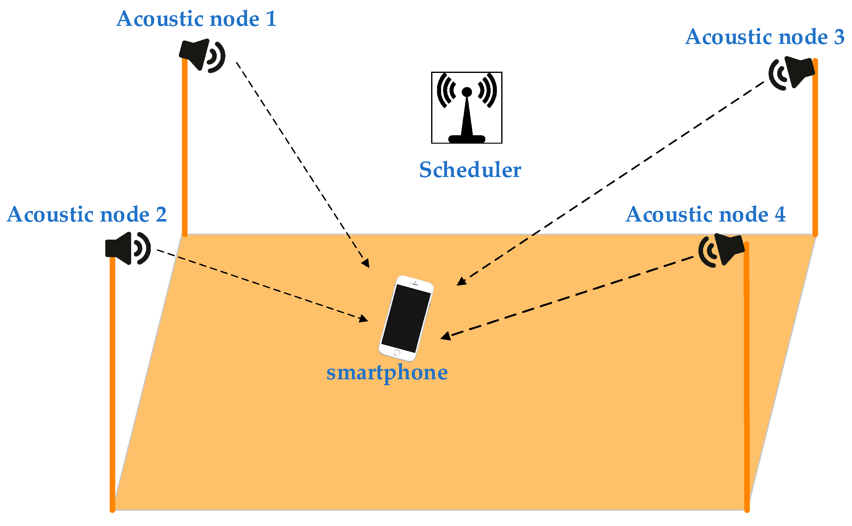
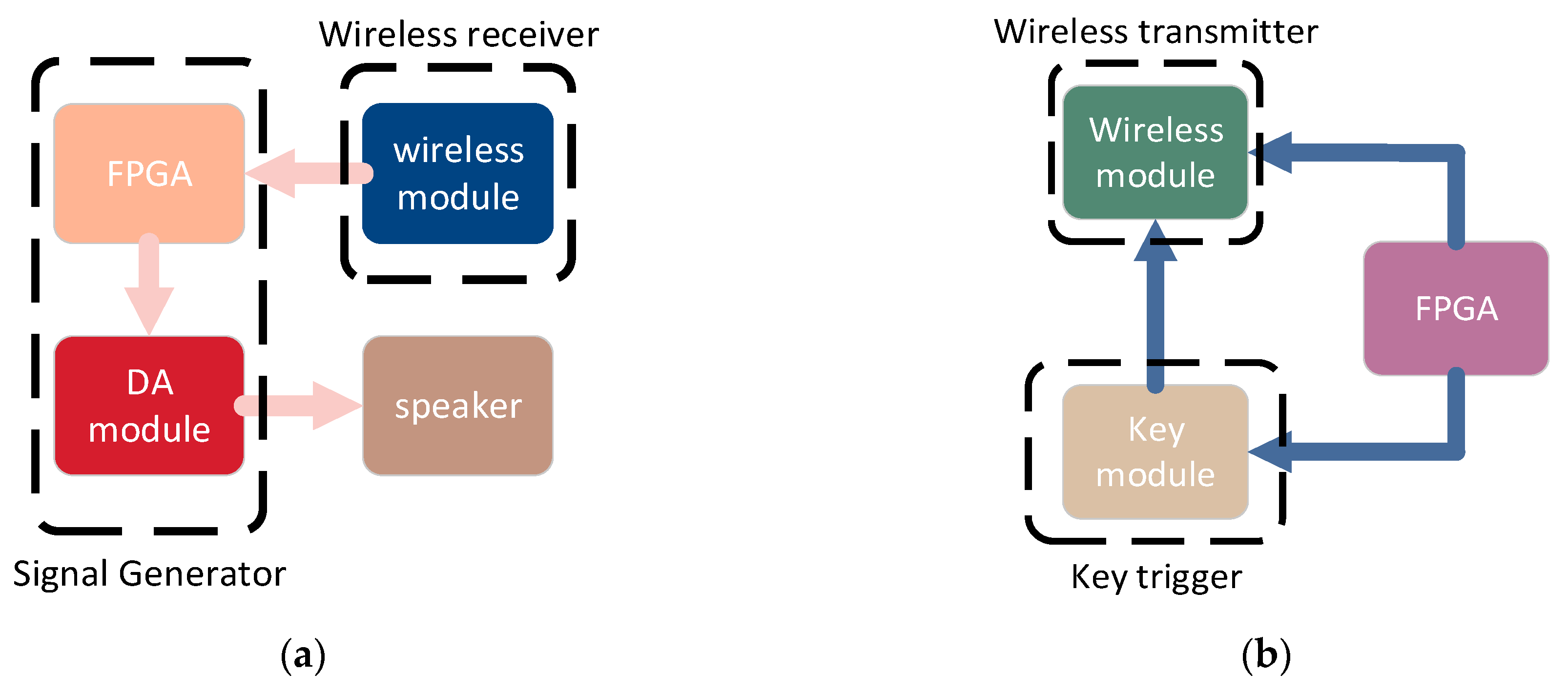
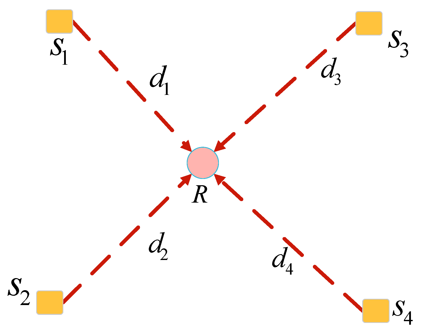
2. Basic Acoustic Positioning System

The acoustic positioning system is composed of a wireless scheduler, acoustic nodes as the signal transmitters and a smartphone as the signal receiver with the localization to be estimated. The wireless scheduler is mainly used to synchronize all acoustic nodes on a unified time axis. The acoustic nodes mainly transmit signals, and the microphone in the smartphone receives the signals transmitted by the acoustic nodes. The hardware architecture of the acoustic node and scheduler is shown in Figure 1 and Figure 2. The acoustic node is composed of a wireless receiver, FPGA, analog-to-digital converter and speaker. The scheduler is mainly composed of FPGA, wireless transmitter, and key module. When the wireless receiver module receives the signaling sent by the scheduler, the FPGA in the acoustic node starts the interrupt arbitration mechanism to drive the speaker to send the signal. The benefits of our system are the following: (1) the acoustic nodes can be easily synchronized within 0.5 milli-second level with the low-cost wireless scheduler. Such synchronization is supportive to achieve the positioning of sub-meter accuracy in the acoustic positioning system. (2) As the acoustic signals are in essence transmitted by broadcasting, there is no limit on the capacity of the receivers, which is beneficial for massive amount of users in large-scale positioning scenarios.

To describe the hardware in more detail, the DAC module is used to convert the digital signal to the output of the analog acoustic signals and drive the speaker into vibrations of the membrane, which are transmitted through the medium of air. The key module is reserved to start or stop the system. The FPGA in the acoustic node has two functions: (1) storing the signal without losing data. (2) controlling and managing different modules.

3. Robust TDOA Measurement Method

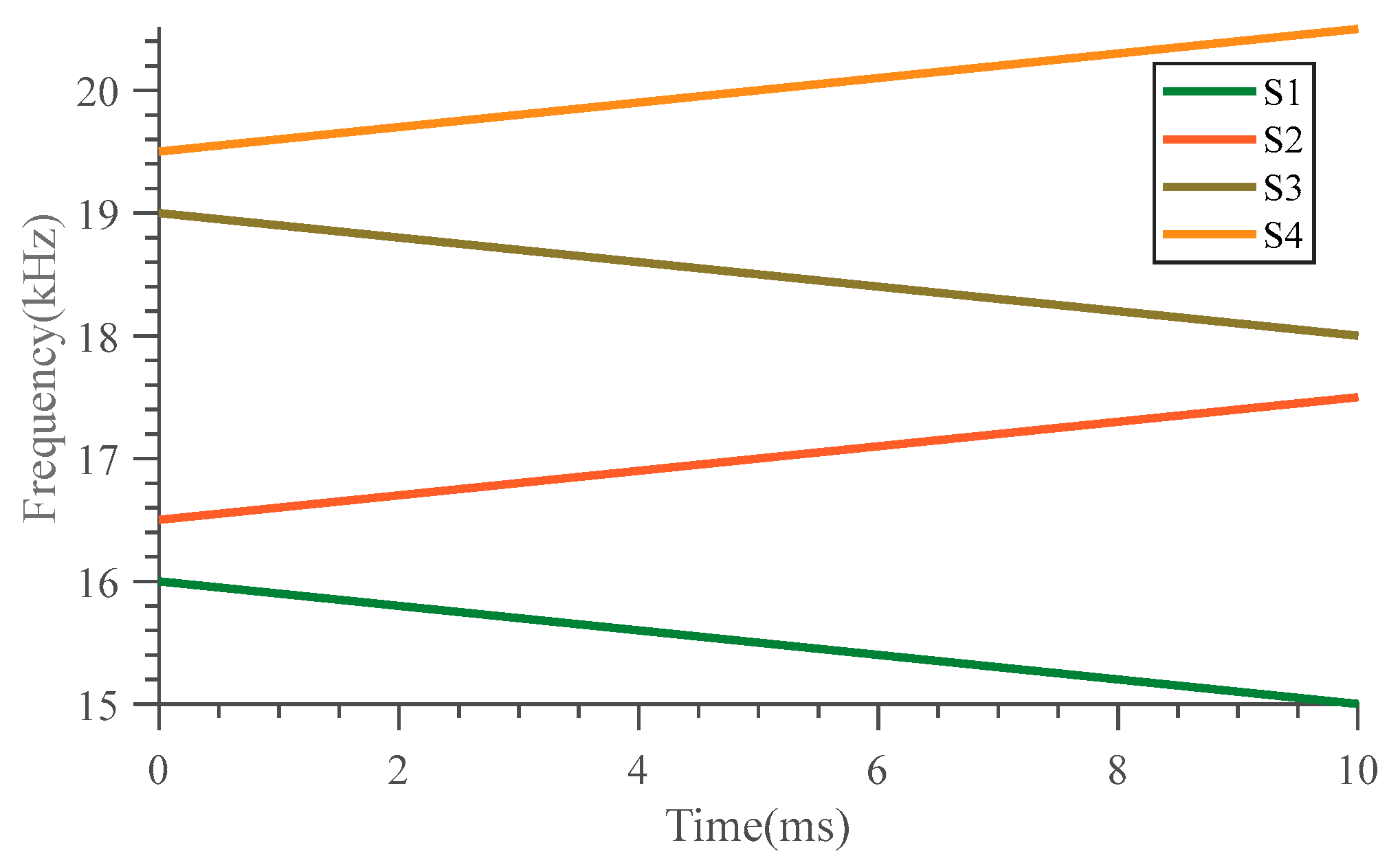
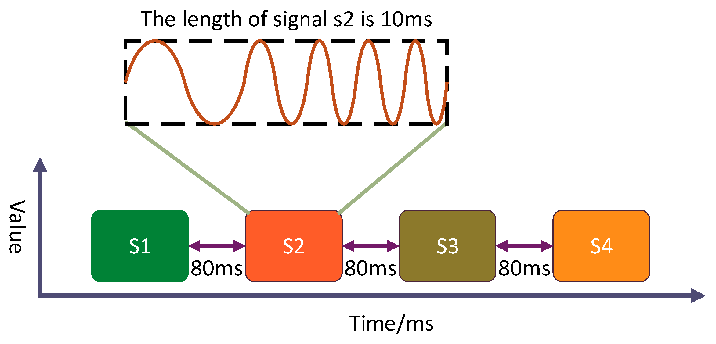
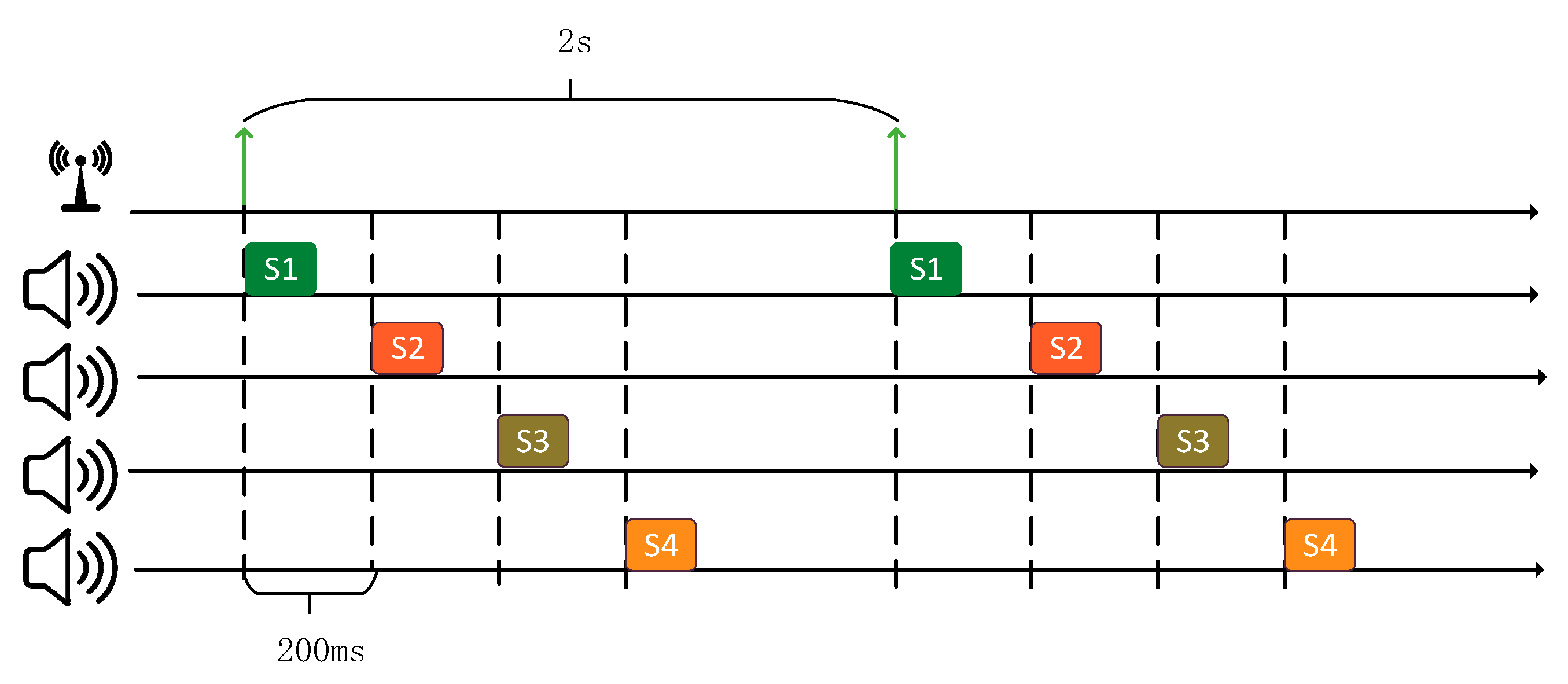
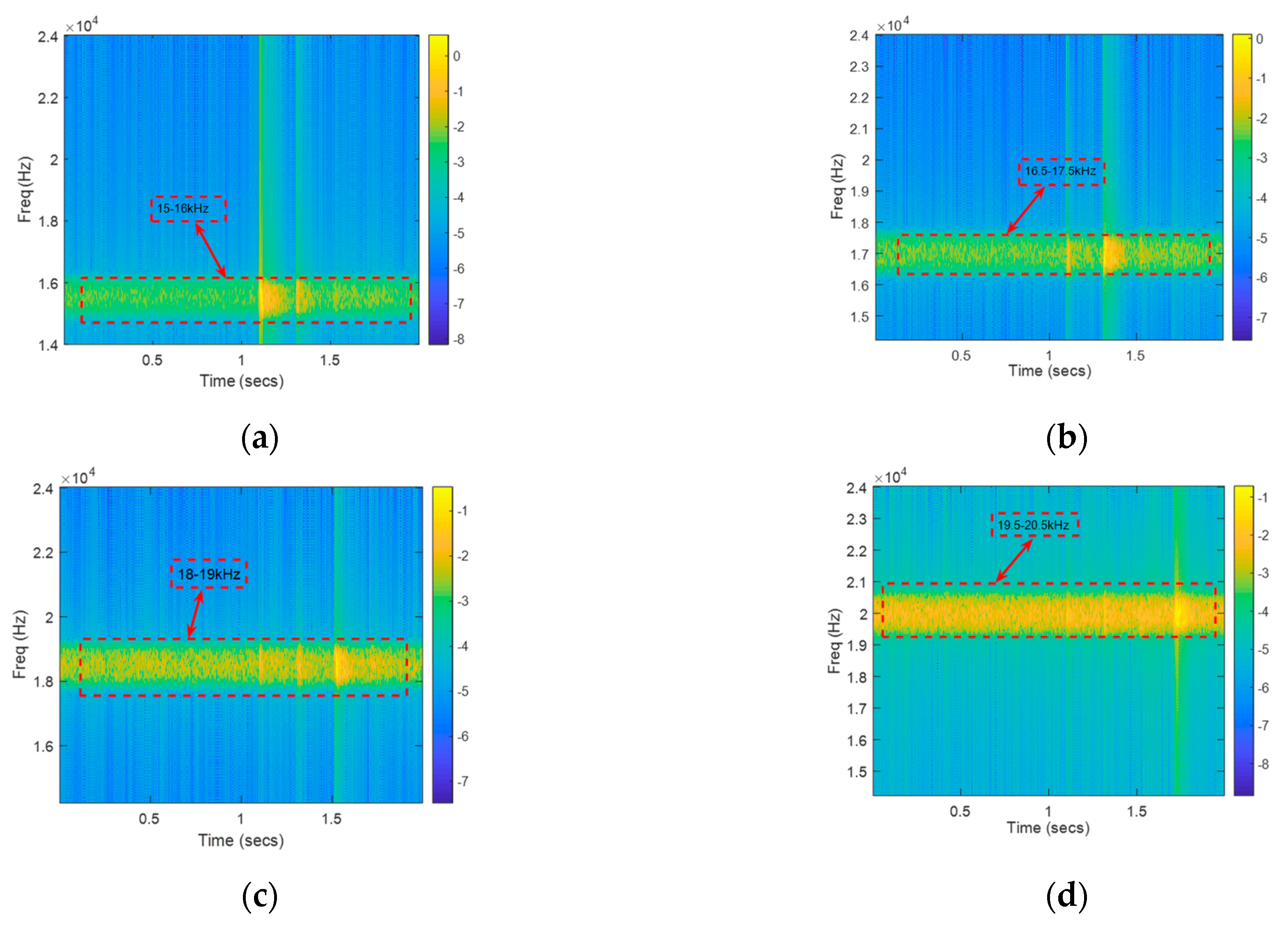
3.1. Signal Design

It has been noted that the chirp signal has good autocorrelation characteristics, which can improve ranging resolution and reception sensitivity. In the meanwhile, the chirp signal can resist a certain degree of multipath fading, and multiple reflected acoustic signals can be distinguished with an appropriate signal processing model. Therefore, we choose the chirp signal as the signal emitted by the acoustic node. chirp signal is defined as follows:

$$\mathrm{s}\left(t\right)=\mathrm{A}{e}^{j(2\mathsf{\pi }(f_{0}t+\frac{f_c-f_0}{2}{t}^2))},0\le t\le \mathrm{T}$$

(1)

where $f_0$ is the starting frequency and $f_c$ is the cut-off frequency. A is the amplitude of the signal. T is the duration of the chirp signal. Let’s make $k=f_c-f_0$. If $k>0$, the chirp signal is up-chirp. If $k<0$, the chirp signal is down-chirp. In order to distinguish four acoustic nodes, we design four chirp signals with different frequency bands. In order to reduce the impact of environmental noise, all acoustic nodes transmit signals with frequencies above 15 kHz. The frequency of the signal transmitted by acoustic node 1 is 16–15 kHz. The frequency of the signal transmitted by acoustic node 2 is 16.5–17.5 kHz. The frequency of the signal transmitted by acoustic node 3 is 19–18 kHz. The frequency of the signal transmitted by acoustic node 4 is 19.5–20.5 kHz.

Figure 3 shows the time-frequency distribution of signals corresponding to each acoustic node. We design chirp signals according to the following principles: (1) up-chirp and down-chirp are distributed in adjacent frequency bands. For example, if s1 is up-chirp, s2 should be down-chirp. If s1 is down-chirp, s2 should be up-chirp. (2) Adjacent coding frequency band interval 500 Hz. (3) The time length of each signal is 10ms to avoid complex calculations. It should be noted that the encoding method in Figure 3 is advantageous for decoding. We only use cross-correlation to detect the received signals. In order to illustrate the effect on decoding by using cross-correlation functions, Figure 4 shows the sequentially received signals defined as s(t), which include s1, s2, s3 and s4.

We use different prior signals (s1, s2, s3, and s4) to correlate with the received signal s(t). After cross-correlation, the signals can be decoded and the time delay of the signals can be estimated as well, which is shown in Figure 5.

In practice, acoustic nodes transmit signals in turn to avoid signal aliasing. All acoustic nodes in this paper can be scheduled by the scheduler for scheduling time. In this paper, the scheduler transmits a wireless trigger signal every two seconds and when the acoustic nodes receive the trigger signal, acoustic nodes transmit chirp signals in turn every 200 ms. The specific scheduling diagram is shown in Figure 6.

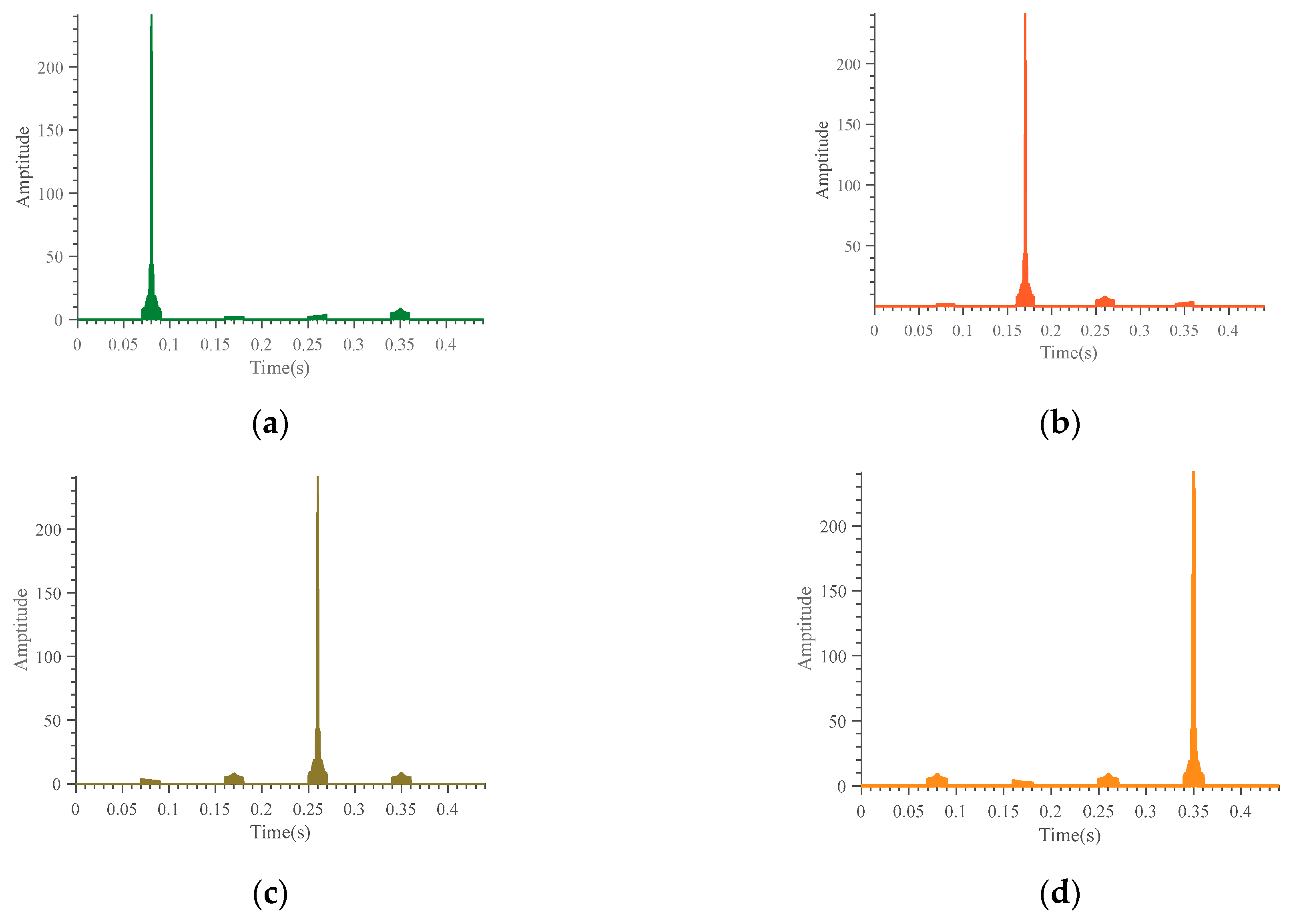
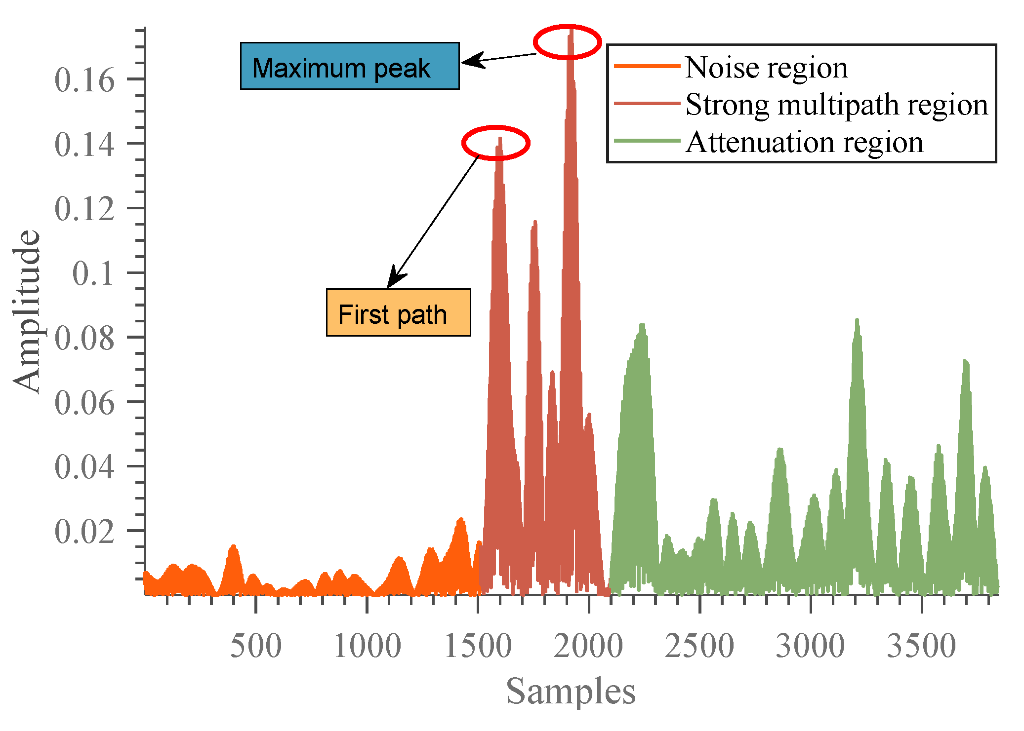
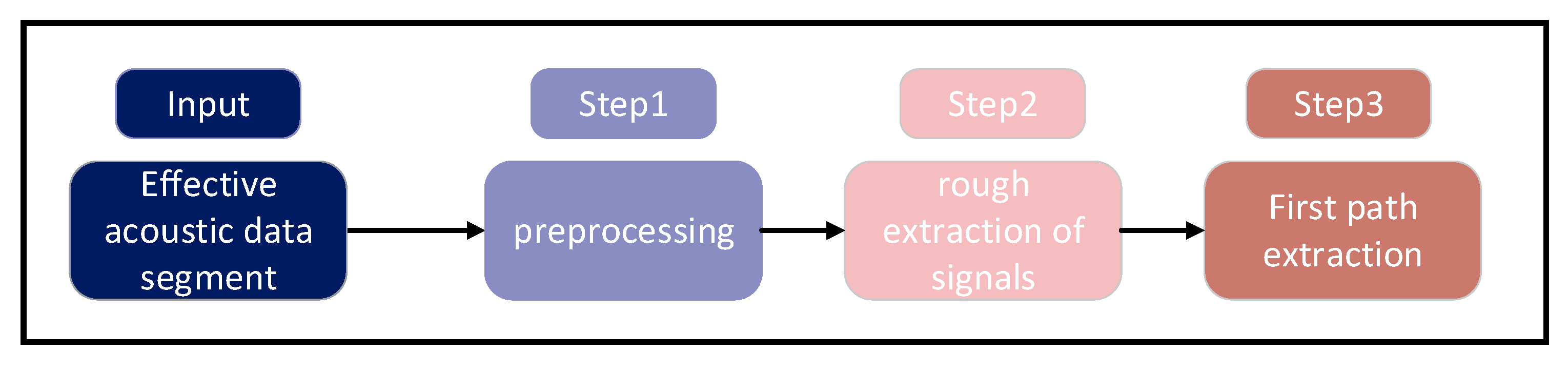
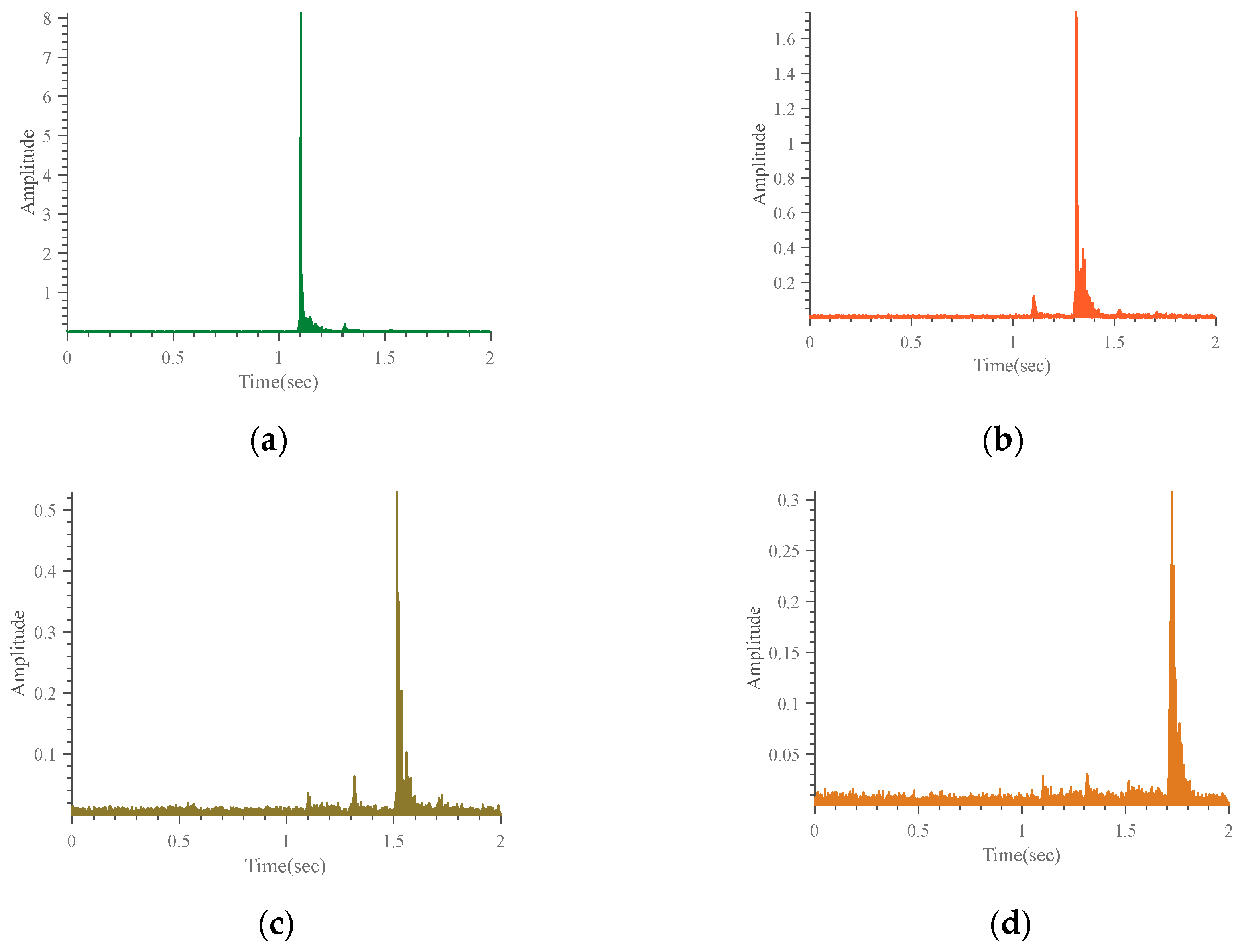
3.2. Robust TDOA Measurement

TOA and TDOA of signals are important parameters of trilateration in indoor positioning. TOA of an acoustic signal refers to the time from the signal sent by the acoustic node to the signal received by the microphone receiver. At present, TOA-based acoustic positioning systems require time synchronization between transmitting nodes and receivers. If TOA can be converted into distance information, the target can be located by the trilateral positioning method. TDOA is the difference in time taken between acoustic signals sent from different sources to the target. TDOA measurement does not require synchronization between acoustic nodes and receivers, only synchronization between acoustic nodes. Therefore, the microphone inside the smartphone can act as a receiver. Similarly, the TDOA can be converted into the distance difference, and then the distance difference is used to realize the target position estimation. The measurement accuracy of TOA and TDOA is the key to ensuring positioning accuracy. However, the signal is reflected by the wall and ground (i.e., multipath effect), and the accuracy of TOA and TDOA estimation is affected in practical applications. Therefore, reliable TDOA estimation is also an important work. As shown in Figure 7, the maximum peak obtained by the correlation operation lags behind the first path due to the influence of the multipath effect. Identifying reflected signals and direct signals is also the key to determining positioning accuracy. Since TDOA does not need the clock synchronization between the mobile phone and the acoustic node, we can use TDOA information to achieve indoor positioning for smartphones.

The benefits of the TDOA positioning system have been described previously. For four acoustic nodes, we can obtain four TOAs. So we can obtain three TDOAs by the following formula:

$$TDO{A}_j=TO{A}_1-TO{A}_{j+1}-0.2\mathrm{s}·j j=1,2,3$$

(2)

According to the above formula, we can know the precondition for obtaining TDOA is to obtain the TOA of the signal. As mentioned above, acoustic signals will be reflected by glass, walls and other obstacles in the environment. Distinguishing reflected signals and direct signals is one of our research works. Based on the multipath problem, we have developed a reliable TOA detection method. The TOA detection process of the acoustic signal is as follows:

In order to obtain the TOA of the corresponding signal emitted by the acoustic node, we follow the process shown in Figure 8. The effective acoustic data segment contains the corresponding signals of all acoustic nodes, and the length of the effective acoustic segment is 2 s. The whole process is divided into three steps, as shown in Figure 8 below.

In step 1, we set four band-pass filters to remove environmental noise and other noise from other acoustic nodes. The four band-pass filters are of finite impulse response type, which is recorded as FIR1, FIR2, FIR3 and FIR4. The band pass range of FIR1 is 15–16 kHz. The band pass range of FIR2 is 16.5–17.5 kHz. The band pass range of FIR3 is 18–19 kHz. The band pass range of FIR4 is 19.5–20.5 kHz. When an effective acoustic segment passes through four filters, four filtered signals are obtained. Four filtered signals are recorded as F1, F2, F3, and F4, respectively.

In step 2, we use the cross-correlation operation to decode the signal and then extract the signal. The cross-correlation calculation formula is as follows:

$$R_i\left(t\right)=\mathrm{abs}\left(F^{-1}\left[F\left[s_d\left(t\right)\right]F^{*}\left[y\left(t\right)\right]\right]\right)$$

(3)

where $R_i\left(t\right)$ is the absolute value of cross correlation result, $s_d\left(t\right)$ is a prior template signal, $y\left(t\right)$ is the received signal, $F$ and $F^{-1}$ are Fourier transform and its inverse transform, respectively, and $F^{*}$ is the complex conjugate of $F$. After the signal is decoded, the signal can be extracted. Rough extraction of the signal is as follows (Algorithm 1):

Algorithm 1. Rough extraction of signal

Input: Filtered signal. Output: Rough extraction of signal. 1: Cross-correlation between filtered signal and different prior signals 2: Based on the step 1, different cross-correlation maximum values are obtained 3: TR is the maximum value among all maximum values in step 2. 4: Decoding decision  if TR corresponds to the signal that needs to be roughly extracted   (1) Find the time $t_{max}^p$ corresponding to TR.   (2) Rough extraction of signal in the time period ($t_{max}^q-40 \mathrm{ms}$, $t_{max}^q+40 \mathrm{ms}$).  else   (1) Find the time $t_{max}^p$ corresponding to TR.   (2) Assigning acoustic data to 0 in the time period ($t_{max}^q-40 \mathrm{ms}$, $t_{max}^q+40 \mathrm{ms}$).   (3) return to step 1.  end if 5: Return: Rough extraction of signal.

In the third step, we use the signal extracted in the second step to perform cross-correlation operations with the prior signal. We obtain the correlation function $R_i\left(t\right)$ through cross-correlation operation. We develop the stable first path extraction method base on $R_i\left(t\right)$. The information of the first path can be converted into TOA information. The first path extraction algorithm is as follows (Algorithm 2):

Algorithm 2. First path extraction

Input: $R_i$. Output: TOA. 1: Set threshold $q$ ($q\in \left[0.3:\mathsf{\delta }:1\right]$, $\mathsf{\delta }$ is the step size) 2: Set $\mathsf{\delta }=0.01$. 3: $\mathsf{\rho }=max\left(R_i\right)$. 4: Find $inde{x}_i\left(n\right)=argmin\left(R_i\ge q\left(n\right)\ast \mathsf{\rho }\right)$, n = 1, 2…71. 5: Group decision:  (1) Set variable GD = 1, GD represents the number of the group.  (2) for n = 1:70        $\mathrm{inteval}\left(n\right)=inde{x}_i\left(n+1\right)-inde{x}_i\left(n\right);$     end for     for n = 1:69        if $\mathrm{inteval}\left(n\right)$< 0.5 ms         $inde{x}_i\left(n\right)BelongstogroupGD;$        else         GD = GD + 1;         $inde{x}_i\left(n+1\right)BelongstogroupGD$;        end if     end for  (3) Find the proportion of $inde{x}_i$ in each group, the proportion is ${\sigma }_i\left(n\right)$, n = 1,2…GD.  (4) Find $\mathrm{VB}=argmin\left({\sigma }_i\left(n\right)\ge 10\%\right)$, n = 1,2…GD. 6: Find TOA: In Group $\mathrm{VB}$, find the first element $inde{x}_i^{VB}\left(1\right)/Fs$ as TOA. (Fs refers to the sampling rate of signal, which is set to 48 kHz in this article.) 7: Return: TOA.

When we obtain four TOAs, we can obtain three TDOAs by Formula (2). Since there are a few abnormal values in the TOA detection process, then TDOA measurement can also be affected. TDOA measurement is the precondition of smartphone positioning, so robust TDOA measurement is very necessary. We have carried out optimization processing to overcome TDOA abnormal measurement. The algorithm is as follows (Algorithm 3):

Algorithm 3. Robust TDOA measurement

Input: TOA1 TOA2 TOA3 TOA4. Output: TDOA1 TDOA2 TDOA3. 1: TDOA calculation  for $j$ = 1:3   $TDO{A}_j=TO{A}_1-TO{A}_{j+1}-j\ast 200\mathrm{ms}$.  end for 2: Set $\mathsf{\epsilon }$. ($\mathsf{\epsilon }$ is the upper limit of abnormality, $\mathsf{\epsilon }$ is set to 40 ms.) 3: Exception elimination  for $j$ = 1:3     if $abs\left(TDO{A}_j\left(1\right)\right)>\mathsf{\epsilon }$      $TDO{A}_j\left(1\right)=min(abs\left(TDO{A}_1\left(1\right)\right) abs\left(TDO{A}_2\left(1\right)\right) abs\left(TDO{A}_3\left(1\right)\right))$.     end if     for n = 1:99      if $TDO{A}_j\left(n+1\right)>\mathsf{\epsilon }$       $TDO{A}_j\left(n+1\right)=TDO{A}_j\left(n\right)$.      end if     end for  end for 4: Return: TDOA1 TDOA2 TDOA3.

In the entire process mentioned above, we can obtain robust TDOA measurements. When the speed of sound is known, we can convert TDOA into distance difference. By using three or more effective TDOA observations, a smartphone can locate its own position.

3.3. Static Robust Positioning Algorithm Base on TODA

Figure 9 represents the fundamental mathematical model utilized in this article. $S_i$ represents the acoustic node $i$. R represents the internal microphone of smartphone. TDOA needs to be converted into distance difference for positioning. The formula is as follows:

$$∆d_i=d_1-d_{i+1}=TDO{A}_i·c i=1,2,3$$

(4)

where c is the speed of sound, c is 340 m/s at 15 centigrade. $∆d_i$ is the distance difference. $d_1$ is the distance from the smartphone to the reference node. In this paper, acoustic node 1 is the reference node. Suppose $r\left(x,y\right)$ is the actual coordinate of the smartphone, and $s_i\left(x_i,y_i\right)$ is the coordinate of the acoustic node. $d_i$ is the distance from the smartphone to the acoustic node $i$. The $d_i$ is calculated as follows:

$$d_i=\sqrt{{\left(x-x_i\right)}^2+{\left(y-y_i\right)}^2} i=1,2,3,4$$

(5)

Substitute Formula (5) into Formula (4) to obtain Formula (6):

$$∆d_i=\sqrt{{\left(x-x_1\right)}^2+{\left(y-y_1\right)}^2}-\sqrt{{\left(x-x_{i+1}\right)}^2+{\left(y-y_{i+1}\right)}^2} i=1,2,3$$

(6)

By assuming that all the anchor positions are known, $p_i$ is the actual measured distance difference, which is related to TDOA measurement. Although we have optimized the TDOA detection algorithm, we cannot completely eliminate the TDOA measurement error. So $p_i$ also include errors.

$$n_i=p_i-∆d_i i=1,2,3$$

(7)

where $n_i$ is the measurement error. In order to establish the relationship between the measured distance difference $p_i$ and the smartphone position $r\left(x,y\right)$, we substitute (5) into (6) to obtain three equations. So, the least squares condition is usually considered to estimate position $R\left(x^{\prime },y^{\prime }\right)$.

$$R=argmin{\displaystyle \sum }_{i=1}^3{\left(p_i-∆d_i\right)}^2$$

(8)

It is easy to see that the problem of solving Formula (8) is a nonlinear problem. In order to observe the performance of positioning algorithms, we carried out a static positioning simulation. We choose two commonly positioned algorithms as the comparison: the Chan method and the ML method. Chan method is a linear estimator that can convert nonlinear problems into linear problems. ML method is a nonlinear estimator, which directly solves optimization problems. These two methods are representative.

We simulate and analyze these two positioning methods to obtain a robust positioning algorithm for two scenes. The first scene is 4.8 m × 4.8 m in size. The second scene is 6.4 m × 7.9 m in size. We set the standard deviation of noise to 1. The distribution of acoustic nodes and test points is shown in Figure 10. In scenario 1, the coordinates of the four acoustic nodes are (0.0 m, 0.0 m), (4.8 m, 0.0 m), (4.8 m, 4.8 m), (0.0 m. 4.8 m). We select the test points A (2.4 m, 2.4 m) in scenario 1. In the simulation of scenario 2, the coordinates of the four acoustic nodes are (0.0 m. 0.0 m), (0.0 m, 6.4 m), (7.9 m, 6.4 m), (7.9 m, 0.0 m). We select the test points B (2.4 m, 4 m) in scenario 2. Simulating 100 times at each test point (A and B). The positioning results of point A and point B are as shown below:

From Figure 10, it can be seen that the positioning accuracy of the Chan method is lower than that of the ML method under the condition that the standard deviation of the noise is 1. Therefore, the Chan method is not used at last. Under the condition that the standard deviation of the noise is set as 1, we make statistics on the positioning results of point A in scenario 1 and B in scenario 2. As shown in Figure 11, we obtained the positioning results by using the ML algorithm.

From Figure 11, it can be seen that the positioning result is affected by Gaussian noise. The ML localization method exhibits high stability with the standard deviation of noise being set as 1. In order to illustrate the problem, we use the ML method to conduct a positioning simulation for 5 test points in scenario 1. The cumulative distribution function (CDF) diagram is as follows:

From Figure 12, static positioning results are relatively stable by using the ML method. So, we chose ML in the static positioning experiment. The positioning error formula used in this article is as follows:

$$\mathrm{PE}=\sqrt{{\left(x-x^{\prime }\right)}^2+{\left(y-y^{\prime }\right)}^2}$$

(9)

where PE is the positioning error, ($x$, $y$) is the true position, and ($x^{\prime }$, $y^{\prime }$) is the estimation.

4. Experiments and Results

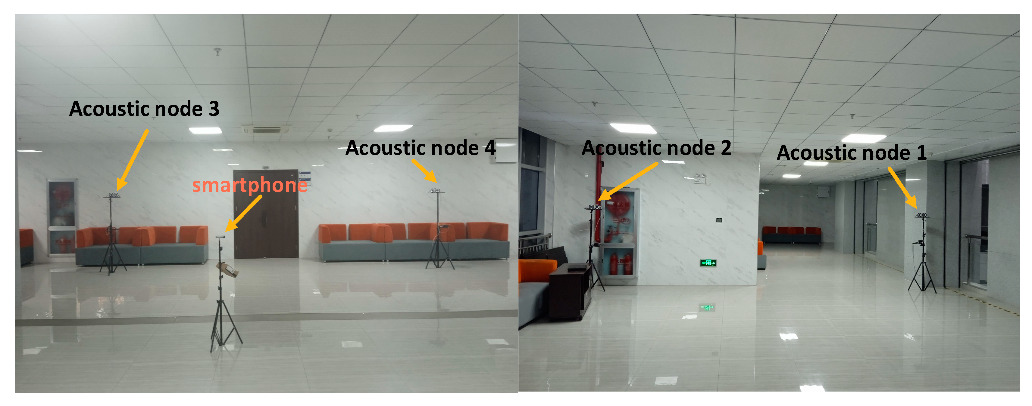
4.1. Experimental Parameters

In this paper, we chose two experimental scenarios. Scenario 1 is in the lounge on the fourth floor of Luojia Laboratory, Wuhan University. Scenario 2 is in the lobby on the second floor of Luojia Laboratory, Wuhan University. The distribution of acoustic nodes and test points in scenario 1 is shown in Figure 12a. The distribution of acoustic nodes and test points in scenario 2 is shown in Figure 13.

In scenario 2, we divide the test point into five areas. In the experiment, the parameters of the experimental signal are designed in advance, and the parameters are shown in

Table 1. Chirp signal parameters of different acoustic nodes.

Acoustic Node	Frequency Range	Signal Type	Duration
node 1	15–16 kHz	down	10 ms
node 2	16.5–17.5 kHz	up	10 ms
node 3	18–19 kHz	down	10 ms
node 4	19.5–20.5 kHz	up	10 ms

:

In two experimental scenarios, the acoustic node deployment shape is rectangular. In Scenario 1, the coordinates of the four acoustic nodes are (0.0 m, 0.0 m, 1.72 m), (0.0 m, 4.8 m, 1.72 m), (4.8 m, 0.0 m, 1.72 m) and (4.8 m, 4.8 m, 1.72 m). In scenario 1, the height of the smartphone is the same as the height of the acoustic nodes. The purpose is to verify the reliability of the algorithm in this paper. In scenario 2, the coordinates of the four acoustic nodes are (0.0 m, 0.0 m, 1.72 m), (0.0 m, 6.4 m, 1.72 m), (7.9 m, 0.0 m, 1.72 m) and (7.9 m, 6.4 m, 1.72 m). In Scenario 2, the height of the smartphone is 1.30 m. The process of deploying acoustic nodes is as follows: First, we adjust the height of the acoustic nodes. Then we use the plumb line to align the square acoustic nodes with the top of the square floor tile. Similarly, we also use the plumb line to align the smartphone with the top of the floor tile. The experimental diagram of scenario 2 is shown in the following Figure 14:

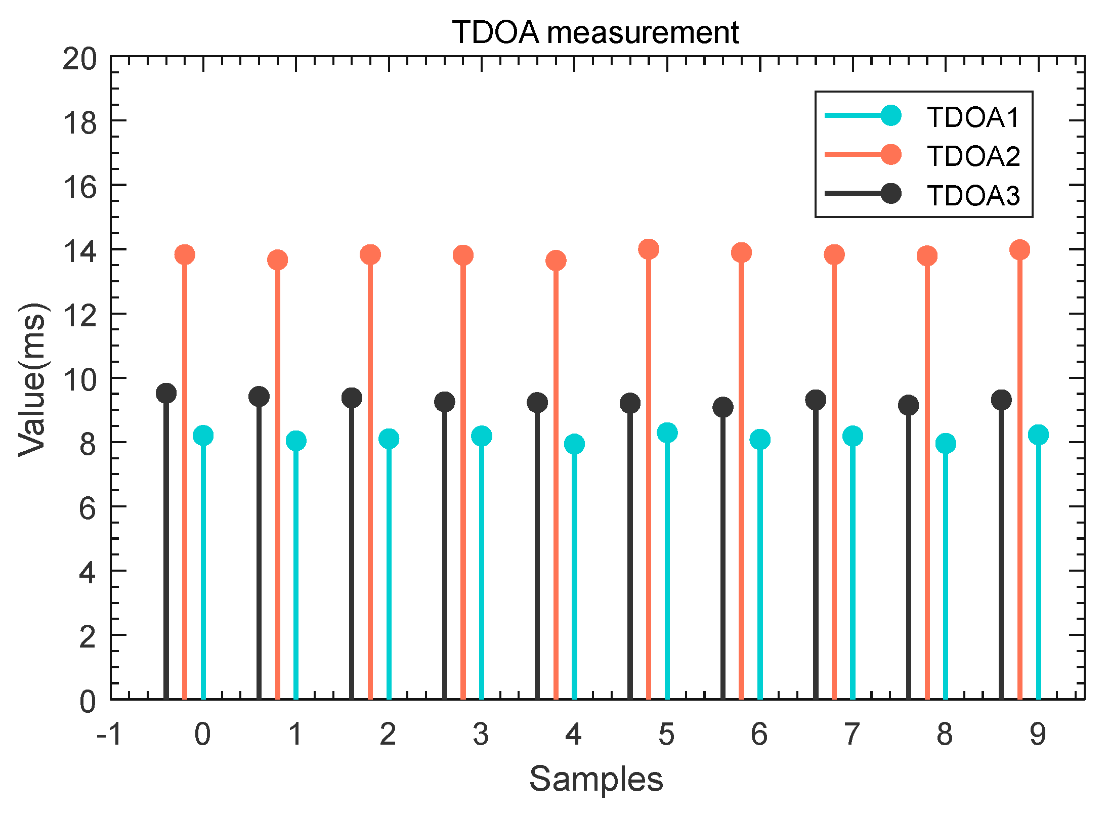
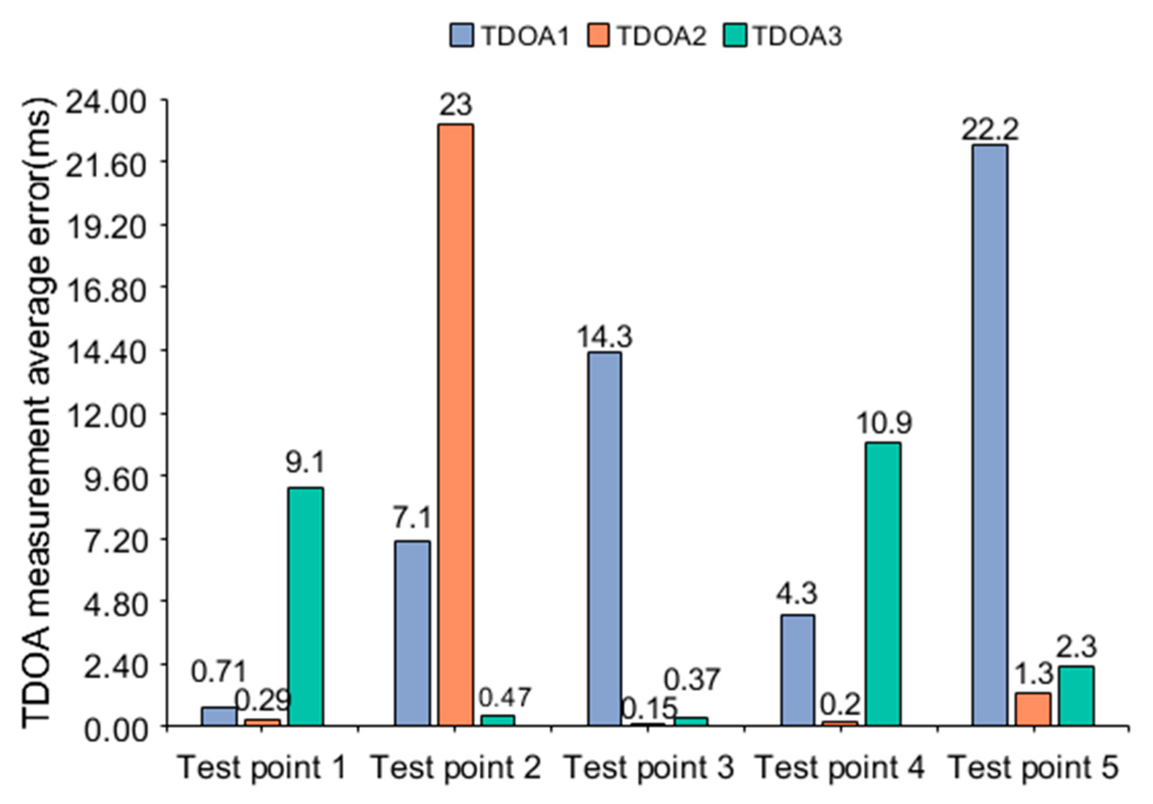
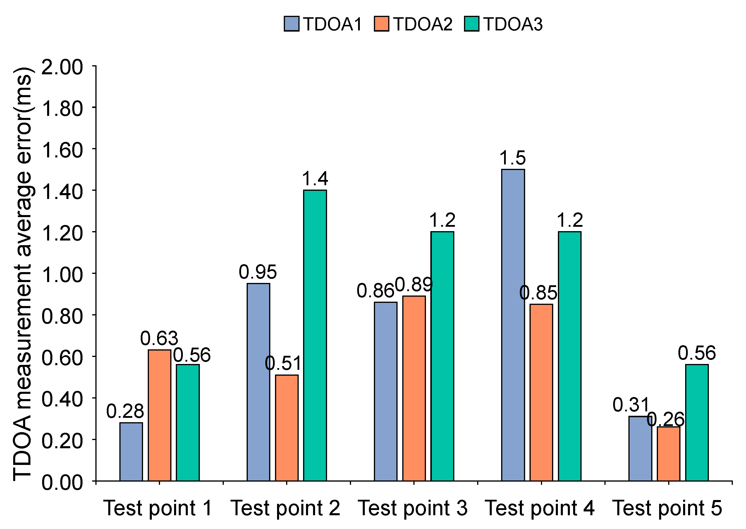
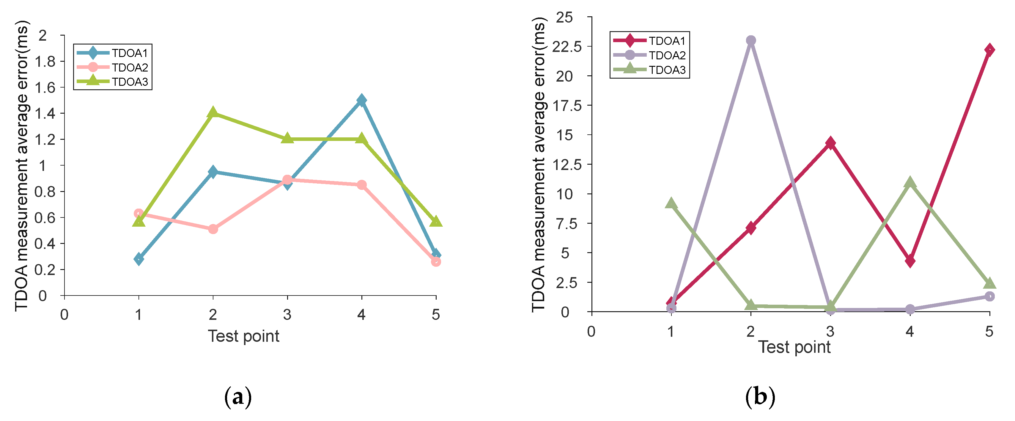
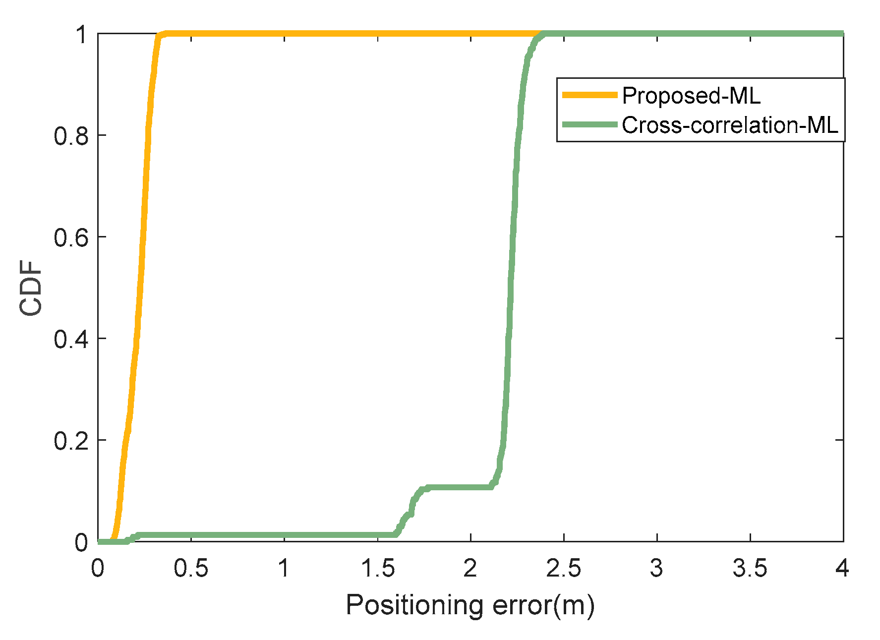
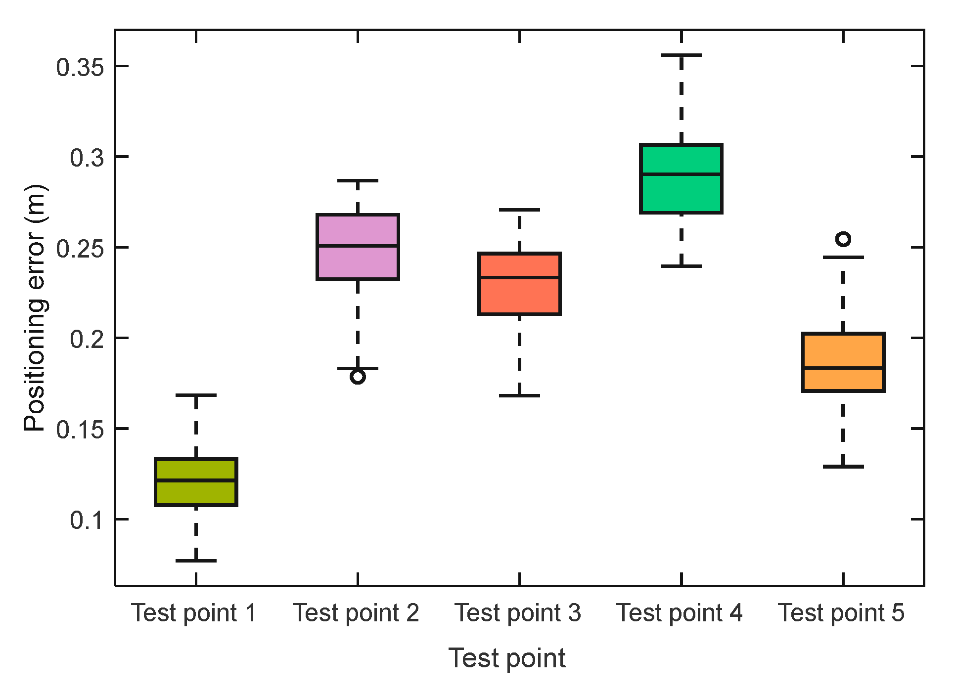
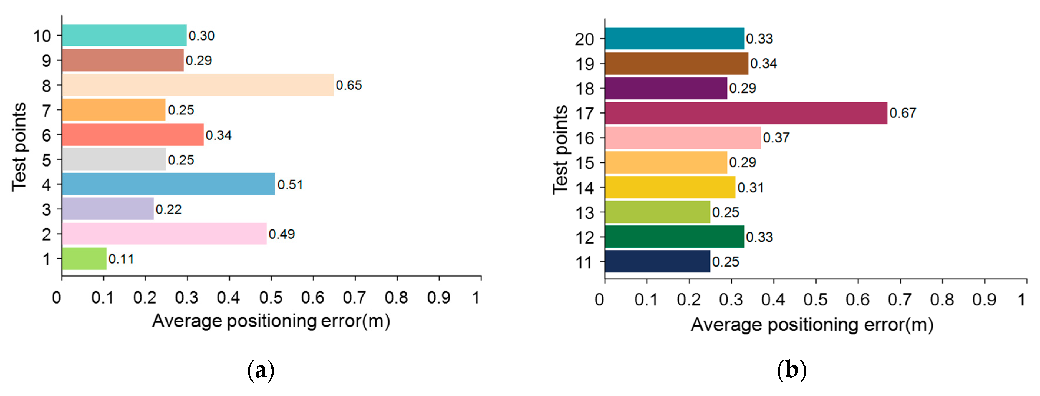
4.2. Experimental Results and Analysis

In the experiment, we used a smartphone to record 5 min acoustic data at each test point. The recorded data will be processed and analyzed with the MATLAB platform. The length of time for each effective acoustic data segment is 2 s. In order to describe the results of each processing stage more vividly, we choose test point C (0.8 m, 4 m) in scenario 1 as an example. First, we set four different filters (FIR1, FIR2, FIR3 and FIR4) to filter the effective acoustic data segment (This process corresponds to step 1 of Figure 8). We can obtain four filtered signals by using four filters. Four filtered signals are obtained, which are recorded as F1, F2, F3 and F4. In order to illustrate the effect of the four filters, we drew the time-frequency diagram.

It can be seen from the above Figure 15, it is not practical by using time-frequency characteristics to distinguish acoustic nodes (fuzzy time-frequency characteristics). It can also be seen from the above Figure 15, it is not practical to use time-frequency characteristics to obtain TDOA information (complex computation). So, we use prior template signals to correlate with the filtered signal (s1 is cross-correlated with F1, s2 is cross-correlated with F2, s3 is cross-correlated with F3, and s4 is cross-correlated with F4). The schematic diagram of the cross-correlation operation is as follows:

From Figure 16, it can be seen that the four signals can be decoded by simple cross-correlation operation. In order to ensure the robustness of decoding, we implement the decoding method by using algorithm 1 in this paper. Algorithm 1 includes not only decoding but also signal extraction (This process corresponds to step 2 of Figure 8). After P1, P2, P3 and P4 are extracted by using Algorithm 1, we use Algorithm 2 for TOA estimation (this process corresponds to step 3 of Figure 8). In the experiment, we obtained 100 results for each test point. To make it easier to see the TDOAs measurement results at test point C, we selected the first 10 TDOA measurement results to display as follows:

From Figure 17, it can be seen that we can obtain three different TDOAs each time. At test point C, the actual TDOAs are 8.7 ms, 13.3 ms, and 8.7 ms, respectively. We can see that our TDOA measurement value is also close to the actual value. The three TDOAs are different due to the different distances between the smartphone and the four acoustic nodes.

In order to further explain the improvement of TDOA measurement accuracy by Algorithms 2 and 3, we use the average of absolute values of TDOA measurement error (simply referred to as TDOA measurement average error) to explain. We assume that the speed of sound propagation is 340 m/s. TDOA error of 1 ms corresponds to a distance error of 34 cm. We draw the TDOA measurement average error histogram as shown in Figure 18 and Figure 19.

From Figure 18, it can be seen that the TDOAs obtained using the cross-correlation algorithm always have large errors. At test point 1, TDOA3 has a large average measurement error. At test point 2, TDOA1 and TDOA2 have large average measurement errors. At test point 3, TDOA1 has a large average measurement error. At test point 4, TDOA3 has a large average measurement error. At test point 5, TDOA1 has a large average measurement error. Therefore, TDOA1, TDOA2, and TDOA3 may all have large errors. When we use the ML algorithm for positioning, divergence occurs (i.e., the positioning result tends to infinity). Hence, stable and reliable TDOA measurements are a prerequisite for positioning. In indoor spaces, there is a phenomenon where the strongest path lags behind the direct path. This phenomenon is the essential reason for the large TDOA measurement errors in Figure 18. We developed Algorithms 2 and 3 to improve the problem of large TDOA measurement errors.

As can be seen from Figure 19, TDOAs measurement average error has significantly decreased compared to Figure 18. In test point 1, the TDOA2 measurement average error is the maximum value (0.6 ms). In test point 2, TDOA3 measurement average error is the maximum value of (1.4 ms). In test point 3, TDOA3 measurement average error is the maximum value (1.2 ms). In test point 4, the TDOA1 measurement average error is the maximum value (1.5 ms). In test point 5, the TDOA3 measurement average error is the maximum value (0.56 ms). All TDOA measurement average errors are less than 1.6 ms (corresponding distance difference error is 54.4 cm), which provides a prerequisite for achieving decimeter-level positioning in scenario 1. When we use the ML algorithm for positioning, the results will be more stable. To further illustrate the better stability of our TDOA measurement method, we will display the data in Figure 18 and Figure 19 by using a line chart.

As can be seen from Figure 20, the proposed method has better stability for TDOA measurement. In Figure 20a, the measurement average error of TDOA1 varies between 0.2 ms and 1.6 ms, the measurement average error of TDOA2 varies between 0.2 ms and 1 ms, and the measurement average error of TDOA3 varies between 0 ms and 1.5 ms. In Figure 20b, the measurement average error of TDOA1 varies between 0 ms and 23 ms, the measurement average error of TDOA2 varies between 0 ms and 23 ms, and the measurement average error of TDOA3 varies between 0 ms and 12 ms. So, it can be seen that the proposed method shows good stability. At the same time, it can be seen that the proposed method has a relatively low measurement error in all TDOA measurements. After we obtain TDOAs, we perform the localization function by using the ML algorithm. We refer to the floor tiles to obtain an approximate true value of the smartphone’s position. Then we calculate the CDF with two methods (Proposed-ML and Cross-correlated-ML), as shown in the following Figure 21.

In Scene 1, we found that the results of using the cross-correlation-ML algorithm for localization at testing points 2 and 4 tend toward infinity. Therefore, in Figure 22, we do not show the localization results for testing points 2 and 4 when using the Cross-correlation-ML method. By using the algorithm proposed in this paper, high-precision localization results were obtained in the localization experiment in Scene 1. In Scene 1, each test point was located 100 times. We used box plots to display the localization results obtained using the proposed algorithm in Scene 1.

As can be seen from Figure 22, the indoor acoustic positioning system was tested using a Proposed-ML algorithm to increase its accuracy to the decimeter level in scenario 1. The preparatory work involved coordinating the acoustic nodes and test points using computer software and calibrating them with a plumb line. In scenario 1, five test points were used, each with known coordinates. These test points were triggered every two seconds by the scheduler, and each point was tested 100 times to increase randomness. The positioning error was evaluated using Formula (9) given in the paper. To verify the accuracy of the system further, data were collected at 20 different test points in scenario 2. Each test point was tested 100 times, and the average positioning error of the 20 test points was shown in Figure 23.

According to Figure 23, the method proposed in this article is still applicable to Scenario 2. In Region 1, the average positioning error of the test points is 0.36 m; in Region 2, the average positioning error of the test points is 0.34 m; in Region 3, the average positioning error of the test points is 0.32 m; in region 4, the average positioning error of the test points is 0.40 m; and in region 5, the average positioning error of the test points is 0.29 m. Therefore, sub-meter-level positioning accuracy can still be achieved in Scenario 2. Our system and method provide a good solution for indoor positioning.

5. Conclusions

This article describes an intelligent smartphone positioning system based on acoustic localization. The encoding scheme we designed is simple, and decoding only requires simple cross-correlation operations. The signal frequency designed in this article is much higher than the frequency of environmental noise. The accuracy and stability of TDOA measurement are greatly affected by multipath effects. Traditional cross-correlation algorithms cannot solve this problem. Based on cross-correlation algorithms, we developed Algorithms 1–3. We not only decoded the acoustic node signals but also obtained stable and high-precision TDOA measurement results. In terms of positioning algorithms, we chose a reliable maximum likelihood algorithm as the basic positioning algorithm. Static positioning experiments were conducted in two scenarios, achieving an average positioning accuracy of decimeter level. In the future, we still need to solve the following problems:

(1)

Large scene smartphone positioning: our acoustic nodes are easy to deploy, and we have the ability to achieve positioning in large indoor spaces. However, there is a problem of near-far effect in large indoor spaces. We plan to overcome this problem using the normalization method.

(2)

Dynamic positioning: acoustic signal is susceptible to Doppler effects. This issue is something we need to address in the future. We plan to choose methods in the field of communication, such as carrier frequency offset compensation.

(3)

Switching between dynamic positioning and static positioning: When performing the positioning function, the user may be in a stationary state or a moving state. In the moving state, we can use an extended Kalman Filter to improve positioning accuracy. We plan to use TOA information to detect movement distance and determine whether it is stationary.

(4)

Adaptive extraction of valid acoustic data segments: this article does not study the adaptive extraction method. However, signals from acoustic nodes can be encoded and decoded, which provides the possibility for adaptive extraction.

(5)

Smartphone outside of the rectangle of four nodes: When the Smartphone is outside the acoustic nodes, fingerprint positioning can be used. In addition, increasing the number of acoustic nodes and using time-division, space-division, and code-division technologies can also achieve localization.

References

1. Liu, M.; Cheng, L.; Qian, K.; Wang, J.; Wang, J.; Liu, Y. Indoor acoustic localization: A survey. Hum. Cent. Comput. Inf. Sci. 2020, 10, 2. [Google Scholar] [CrossRef]
2. Lee, M.J.L.; Hsu, L.-T.; Ng, H.-F. Semantic VPS for smartphone localization in challenging urban environments. Sensors 2021, 21, 6137. [Google Scholar] [CrossRef]
3. Bi, J.; Zhao, M.; Yao, G.; Cao, H.; Feng, Y.; Jiang, H.; Chai, D. PSOSVRPos: WiFi indoor positioning using SVR optimized by PSO. Expert Syst. Appl. 2023, 222, 119778. [Google Scholar] [CrossRef]
4. Peng, P.; Yu, C.; Xia, Q.; Zheng, Z.; Zhao, K.; Chen, W. An Indoor Positioning Method Based on UWB and Visual Fusion. Sensors 2022, 22, 1394. [Google Scholar] [CrossRef]
5. Zafari, F.; Gkelias, A.; Leung, K.K. A survey of indoor localization systems and technologies. IEEE Commun. Surv. Tutor. 2019, 21, 2568–2599. [Google Scholar] [CrossRef] [Green Version]
6. Yeh, S.-C.; Hsu, W.-H.; Lin, W.-Y.; Wu, Y.-F. Study on an indoor positioning system using Earth’s magnetic field. IEEE Trans. Instrum. Meas. 2019, 69, 865–872. [Google Scholar] [CrossRef]
7. Huang, B.; Xu, Z.; Jia, B.; Mao, G. An online radio map update scheme for WiFi fingerprint-based localization. IEEE Internet Things J. 2019, 6, 6909–6918. [Google Scholar] [CrossRef]
8. Han, K.; Yu, S.M.; Kim, S.-L.; Ko, S.-W. Exploiting user mobility for WiFi RTT positioning: A geometric approach. IEEE Internet Things J. 2021, 8, 14589–14606. [Google Scholar] [CrossRef]
9. Yu, Y.; Chen, R.; Chen, L.; Guo, G.; Ye, F.; Liu, Z. A robust dead reckoning algorithm based on Wi-Fi FTM and multiple sensors. Remote Sens. 2019, 11, 504. [Google Scholar] [CrossRef] [Green Version]
10. Banin, L.; Bar-Shalom, O.; Dvorecki, N.; Amizur, Y. Scalable Wi-Fi client self-positioning using cooperative FTM-sensors. IEEE Trans. Instrum. Meas. 2018, 68, 3686–3698. [Google Scholar] [CrossRef]
11. Kumar, S.; Kaltenberger, F.; Ramirez, A.; Kloiber, B. An SDR implementation of WiFi receiver for mitigating multiple co-channel ZigBee interferers. EURASIP J. Wirel. Commun. Netw. 2019, 2019, 224. [Google Scholar] [CrossRef] [Green Version]
12. Alavi, B.; Pahlavan, K. Modeling of the TOA-based distance measurement error using UWB indoor radio measurements. IEEE Commun. Lett. 2006, 10, 275–277. [Google Scholar] [CrossRef]
13. Pfeil, R.; Pichler, M.; Schuster, S.; Hammer, F. Robust acoustic positioning for safety applications in underground mining. IEEE Trans. Instrum. Meas. 2015, 64, 2876–2888. [Google Scholar] [CrossRef]
14. Oloumi, D.; Rambabu, K. Metal-cased oil well inspection using near-field UWB radar imaging. IEEE Trans. Geosci. Remote Sens. 2018, 56, 5884–5892. [Google Scholar] [CrossRef]
15. Zhang, W.; Chowdhury, M.S.; Kavehrad, M. Asynchronous indoor positioning system based on visible light communications. Opt. Eng. 2014, 53, 045105. [Google Scholar] [CrossRef]
16. Yasir, M.; Ho, S.-W.; Vellambi, B.N. Indoor positioning system using visible light and accelerometer. J. Light. Technol. 2014, 32, 3306–3316. [Google Scholar] [CrossRef]
17. Jung, S.-Y.; Hann, S.; Park, C.-S. TDOA-based optical wireless indoor localization using LED ceiling lamps. IEEE Trans. Consum. Electron. 2011, 57, 1592–1597. [Google Scholar] [CrossRef]
18. Yang, S.-H.; Kim, H.-S.; Son, Y.-H.; Han, S.-K. Three-dimensional visible light indoor localization using AOA and RSS with multiple optical receivers. J. Light. Technol. 2014, 32, 2480–2485. [Google Scholar] [CrossRef]
19. Alam, F.; Chew, M.T.; Wenge, T.; Gupta, G.S. An accurate visible light positioning system using regenerated fingerprint database based on calibrated propagation model. IEEE Trans. Instrum. Meas. 2018, 68, 2714–2723. [Google Scholar] [CrossRef]
20. Xie, C.; Guan, W.; Wu, Y.; Fang, L.; Cai, Y. The LED-ID detection and recognition method based on visible light positioning using proximity method. IEEE Photonics J. 2018, 10, 7902116. [Google Scholar] [CrossRef]
21. Abou-Shehada, I.M.; AlMuallim, A.F.; AlFaqeh, A.K.; Muqaibel, A.H.; Park, K.-H.; Alouini, M.-S. Accurate Indoor Visible Light Positioning Using a Modified Pathloss Model with Sparse Fingerprints. J. Light. Technol. 2021, 39, 6487–6497. [Google Scholar] [CrossRef]
22. Lee, S.; Chae, S.; Han, D. ILoA: Indoor localization using augmented vector of geomagnetic field. IEEE Access 2020, 8, 184242–184255. [Google Scholar] [CrossRef]
23. Ashraf, I.; Din, S.; Hur, S.; Kim, G.; Park, Y. Empirical Overview of Benchmark Datasets for Geomagnetic Field-Based Indoor Positioning. Sensors 2021, 21, 3533. [Google Scholar] [CrossRef] [PubMed]
24. Sun, M.; Wang, Y.; Xu, S.; Yang, H.; Zhang, K. Indoor geomagnetic positioning using the enhanced genetic algorithm-based extreme learning machine. IEEE Trans. Instrum. Meas. 2021, 70, 2508611. [Google Scholar] [CrossRef]
25. Sertatıl, C.; Altınkaya, M.A.; Raoof, K. A novel acoustic indoor localization system employing CDMA. Digit. Signal Process. 2012, 22, 506–517. [Google Scholar] [CrossRef] [Green Version]
26. Liu, Z.; Chen, R.; Ye, F.; Guo, G.; Li, Z.; Qian, L. Improved TOA estimation method for acoustic ranging in a reverberant environment. IEEE Sens. J. 2020. [CrossRef]
27. Cai, C.; Hu, M.; Ma, X.; Peng, K.; Liu, J. Accurate Ranging on Acoustic-Enabled IoT Devices. IEEE Internet Things J. 2019, 6, 3164–3174. [Google Scholar] [CrossRef]
28. Cai, C.; Hu, M.; Cao, D.; Ma, X.; Li, Q.; Liu, J. Self-deployable indoor localization with acoustic-enabled IoT devices exploiting participatory sensing. IEEE Internet Things J. 2019, 6, 5297–5311. [Google Scholar] [CrossRef]
29. Bordoy, J.; Schindelhauer, C.; Höflinger, F.; Reindl, L.M. Exploiting acoustic echoes for smartphone localization and microphone self-calibration. IEEE Trans. Instrum. Meas. 2019, 69, 1484–1492. [Google Scholar] [CrossRef]
30. Zhang, L.; Chen, M.; Wang, X.; Wang, Z. TOA estimation of chirp signal in dense multipath environment for low-cost acoustic ranging. IEEE Trans. Instrum. Meas. 2018, 68, 355–367. [Google Scholar] [CrossRef]
31. Song, X.; Wang, M.; Qiu, H.; Li, K.; Ang, C. Auditory scene analysis-based feature extraction for indoor subarea localization using smartphones. IEEE Sens. J. 2019, 19, 6309–6316. [Google Scholar] [CrossRef]
32. Aguilera, T.; Aranda, F.J.; Parralejo, F.; Gutiérrez, J.D.; Moreno, J.A.; Álvarez, F.J. Noise-Resilient Acoustic Low Energy Beacon for Proximity-Based Indoor Positioning Systems. Sensors 2021, 21, 1703. [Google Scholar] [CrossRef]
33. Chen, X.; Chen, Y.; Cao, S.; Zhang, L.; Zhang, X.; Chen, X. Acoustic Indoor Localization System Integrating TDMA+FDMA Transmission Scheme and Positioning Correction Technique. Sensors 2019, 19, 2353. [Google Scholar] [CrossRef] [PubMed] [Green Version]
34. Qiu, Y.; Li, B.; Huang, J.; Jiang, Y.; Wang, B.; Huang, Z. An Analytical Method for 3-D Sound Source Localization Based on a Five-Element Microphone Array. IEEE Trans. Instrum. Meas. 2022, 71, 7504314. [Google Scholar] [CrossRef]
35. Chung, M.-A.; Chou, H.-C.; Lin, C.-W. Sound Localization Based on Acoustic Source Using Multiple Microphone Array in an Indoor Environment. Electronics 2022, 11, 890. [Google Scholar] [CrossRef]
36. Xing, H.; Yang, X. Sound source localization fusion algorithm and performance analysis of a three-plane five-element microphone array. Appl. Sci. 2019, 9, 2417. [Google Scholar] [CrossRef] [Green Version]
37. Manamperi, W.; Abhayapala, T.D.; Zhang, J.; Samarasinghe, P.N. Drone audition: Sound source localization using on-board microphones. IEEE/ACM Trans. Audio Speech Lang. Process. 2022, 30, 508–519. [Google Scholar] [CrossRef]
38. Go, Y.-J.; Choi, J.-S. An acoustic source localization method using a drone-mounted phased microphone array. Drones 2021, 5, 75. [Google Scholar] [CrossRef]
39. Wang, S.; Yang, P.; Sun, H. Sound Source Localization Indoors Based on Two-Level Reference Points Matching. Appl. Sci. 2022, 12, 9956. [Google Scholar] [CrossRef]
40. Liu, Z.Y.; Chen, R.Z.; Ye, F.; Guo, G.Y.; Li, Z.; Qian, L. Time-of-arrival estimation for smartphones based on built-in microphone sensor. Electron. Lett. 2020, 56, 1280–1283. [Google Scholar] [CrossRef]
41. Toru, I.; Yasuda, Y.; Sato, S.; Izumi, S.; Kawaguchi, H. Millimeter-Precision Ultrasonic DSSS Positioning Technique with Geometric Triangle Constraint. IEEE Sens. J. 2022, 22, 16202–16211. [Google Scholar] [CrossRef]
Figure 1. Acoustic positioning system for smartphone.
Futureinternet 15 00240 g001
Figure 2. Hardware frame diagram (a) Acoustic node hardware architecture; (b) Scheduler hardware architecture.
Futureinternet 15 00240 g002
Figure 3. Time-frequency distribution of different coded chirp signals.
Futureinternet 15 00240 g003
Figure 4. Schematic diagram of combined signal.
Futureinternet 15 00240 g004
Figure 5. Decoding by using cross-correlation operation: (a) s1 is cross-correlated with the combined signal; (b) s2 is cross-correlated with the combined signal; (c) s3 is cross-correlated with the combined signal; (d) s4 is cross-correlated with the combined signal.
Futureinternet 15 00240 g005
Figure 6. Scheduling scheme of acoustic nodes.
Futureinternet 15 00240 g006
Figure 7. Multipath effects of chirp signal.
Futureinternet 15 00240 g007
Figure 8. TOA detection process of acoustic signal.
Futureinternet 15 00240 g008
Figure 9. Mathematical model of positioning.
Futureinternet 15 00240 g009
Figure 10. Comparison of CHAN method and ML method: (a) positioning result of point A by using Chan method and ML method; (b) positioning result of point B by using Chan method and ML method.
Futureinternet 15 00240 g010
Figure 11. Positioning results of point A and point B (using ML method): (a) Positioning results of different elements of test point A; (b) Positioning results of different elements of test point B.
Futureinternet 15 00240 g011
Figure 12. Positioning simulation of scenario 1: (a) distribution of acoustic nodes and test points in scenario 1; (b) the CDF diagram of scenario 1.
Futureinternet 15 00240 g012
Figure 13. Distribution of acoustic nodes and test points in scenario 2.
Futureinternet 15 00240 g013
Figure 14. Experiment scenario 2 diagram.
Futureinternet 15 00240 g014
Figure 15. Time-frequency distribution after using different filters. (a) Time-frequency distribution of F1; (b) Time-frequency distribution of F2; (c) Time-frequency distribution of F3; (d) Time-frequency distribution of F4.
Futureinternet 15 00240 g015
Figure 16. Cross-correlation operation between prior signals and filtered signals: (a) s1 is cross-correlated with F1; (b) s2 is cross-correlated with F2; (c) s3 is cross-correlated with F3; (d) s4 is cross-correlated with F4.
Futureinternet 15 00240 g016
Figure 17. TDOAs measurement results for the first time to ten times at test point C.
Futureinternet 15 00240 g017
Figure 18. TDOA measurement average error in scenario 1 (using cross-correlation).
Futureinternet 15 00240 g018
Figure 19. TDOA measurement average error in scenario 1 (using Algorithms 2 and 3).
Futureinternet 15 00240 g019
Figure 20. TDOA measurement average error in scenario 1: (a) TDOA measurement average error using the proposed algorithm; (b) TDOA measurement average error using the cross-correlation algorithm.
Futureinternet 15 00240 g020
Figure 21. CDF of the positioning errors in the scenario 1.
Futureinternet 15 00240 g021
Figure 22. Box diagram of positioning error at different test points in scenario 1 (using Proposed-ML algorithm).
Futureinternet 15 00240 g022
Figure 23. Average positioning error in scenario 2 (using Proposed-ML algorithm): (a) Average positioning error of test points 1–10; (b) Average positioning error of test points 11–20.
Futureinternet 15 00240 g023