Hybridizing Fuzzy String Matching and Machine Learning for Improved Ontology Alignment

Abstract

Ontology alignment has become an important process for identifying similarities and differences between ontologies, to facilitate their integration and reuse. To this end, fuzzy string-matching algorithms have been developed for strings similarity detection and have been used in ontology alignment. However, a significant limitation of existing fuzzy string-matching algorithms is their reliance on lexical/syntactic contents of ontology only, which do not capture semantic features of ontologies. To address this limitation, this paper proposed a novel method that hybridizes fuzzy string-matching algorithms and the Deep Bidirectional Transformer (BERT) deep learning model with three machine learning regression classifiers, namely, K-Nearest Neighbor Regression (kNN), Decision Tree Regression (DTR), and Support Vector Regression (SVR), to perform the alignment of ontologies. The use of the kNN, SVR, and DTR classifiers in the proposed method resulted in the building of three similarity models (SM), encoded SM-kNN, SM-SVR, and SM-DTR, respectively. The experiments were conducted on a dataset obtained from the anatomy track in the Ontology Alignment and Evaluation Initiative 2022 (OAEI 2022). The performances of the SM-kNN, SM-SVR, and SM-DTR models were evaluated using various metrics including precision, recall, F1-score, and accuracy at thresholds 0.70, 0.80, and 0.90, as well as error rates and running times. The experimental results revealed that the SM-SVR model achieved the best recall of 1.0, while the SM-DTR model exhibited the best precision, accuracy, and F1-score of 0.98, 0.97, and 0.98, respectively. Furthermore, the results showed that the SM-kNN, SM-SVR, and SM-DTR models outperformed state-of-the-art alignment systems that participated in the OAEI 2022 challenge, indicating the superior capability of the proposed method.

1. Introduction

Ontologies are the fundamental building blocks of the semantic web, an emerging field of Artificial Intelligence (AI) that seeks to integrate data and information in a formalized manner [1], allowing for automated understanding and discovery of connections between them. An ontology is an explicit specification of a shared conceptualization [2], serving as a container for knowledge in a specific domain where the relationships between concepts of the ontology are explicitly defined. By providing a standard vocabulary and formal structure for data representation, ontologies enable the reuse and sharing of knowledge across different applications and domains. As such, ontologies play a critical role in advancing the state-of-the-art in real-world applications.

Many ontologies have been developed in diverse domains, including disease [3], agriculture and the Internet of Things [4], smart home design [5], climate change [6], and more [7,8,9,10]; these existing ontologies constitute a wealth of valuable assets available for reuse. The practice of ontology reuse involves leveraging existing ontologies to construct new ones within the same or related domains. To this end, researchers have defined a common framework for ontology reuse that involves ontology selection and ranking, followed by ontology alignment, integration, and/or merging, and finally, evaluation of the new constructed ontology [11,12].

Given the wide array of ontologies available in various domains of knowledge with heterogeneous structures and vocabularies, reusing them is a daunting task that requires meticulous and precise comparisons to identify overlapping and differences between them. This is where ontology alignment, also known as ontology matching, plays a crucial role. However, the challenges inherent in the reuse process are also reflected in ontology alignment [13,14,15,16], given that ontologies are developed independently by different knowledge engineers, each with their unique perspectives. Therefore, a holistic approach must be taken when aligning ontologies, accounting for variations in vocabulary, concept semantics, and structures. Despite numerous efforts to develop effective ontology alignment methods, such as in the Ontology Alignment Evaluation Initiative (OAEI), challenges persist, making it a fascinating and active area of research.

A range of metrics have been proposed for ontology alignment, including lexical, structure-based, and semantic metrics [15,17]. Fuzzy string-matching algorithms and other string matching techniques have been shown to be effective for lexical alignment in several studies [18,19]. However, these methods may not be sufficient on their own, as they do not consider the semantic features of ontologies, especially when concepts are linguistically different but represent the same underlying knowledge, such as acronyms and synonyms. Additionally, some machine learning-based methods used for ontology selection and alignment such as Word2Vec and Skip-gram are not able to recognize previously unseen vocabulary [20,21]. Some studies have proposed structure-based methods for ontology alignment [22,23,24], but these are limited by the different goals and purposes of the design of the target ontologies [23]. Many studies have also made use of external information (meta-data) of the ontology in their methods and graphs for ontology matching to overcome the issue of the complexity of semantic relationships between concepts [25,26,27,28]. Other authors have proposed metrics that combine both semantic and syntactic measures [13,29,30]. However, they have limited performance compared to existing state-of-the-art alignment systems such as the AML [31] and LogMap [32], which participated in the OAEI 2022 challenge.

To address the shortcomings of existing ontology alignment techniques, this study proposed a novel method that hybridizes fuzzy string-matching algorithms with the BERT deep learning model to achieve improved ontology alignment results. Unlike existing fuzzy string-matching algorithms, the proposed method incorporates both the lexical/syntactic and semantic features of ontologies in the alignment process. This was achieved by combining the similarity scores obtained from four fuzzy string-matching algorithms, including the Longest Common Subsequence (LCS), Levenshtein, Jaccard, and Jaro–Winkler, and the similarity scores of the BERT deep learning model with three machine learning regression classifiers including kNN, SVR, and DTR. The aim of the method was to combine the lexical contents of ontologies and the context and semantic properties of ontologies, processed by the fuzzy string-matching algorithms and the BERT model, respectively, for comprehensive and improved ontology alignment performance based on machine learning. The use of the kNN, SVR, and DTR classifiers in the proposed method resulted in the building of three hybrid models, namely, SM-kNN, SM-SVR, and SM-DTR. The experiments were conducted on a dataset obtained from the anatomy track in the OAEI 2022 challenge. The SM-kNN, SM-SVR, and SM-DTR models were trained using the similarity scores obtained by the fuzzy string-matching algorithms and the BERT model for each pair of classes in the input ontologies, as well as the similarity scores obtained by the AML reference alignment system for the same input ontologies. The performances of the SM-kNN, SM-SVR, and SM-DTR models were evaluated using various metrics including precision, recall, F1-score, and accuracy at thresholds 0.70, 0.80, and 0.90, as well as error rates and running times. The experimental results revealed that the SM-SVR model achieved the best recall of 1.0, while the SM-DTR model exhibited the best precision, accuracy, and F1-score of 0.98, 0.97, and 0.98, respectively. Furthermore, the results showed that the SM-kNN, SM-SVR, and SM-DTR models outperformed state-of-the-art alignment systems that participated in the OAEI 2022 ontology alignment challenge, indicating the superior capability of the proposed method.

The main contributions of this study are three-fold:

• The development of a novel method that considers both the lexical and semantic features of ontologies in the alignment process to address the limitations of fuzzy string-matching algorithms,
• The use of deep learning and machine learning regression models to improve ontology alignment results, thereby demonstrating the potential of machine learning in enhancing performance in the field of ontology alignment, and
• The accomplishment of a thorough and detailed performance analysis of the proposed method against state-of-the-art alignment systems in the OAEI 2022 ontology alignment challenge.

The remaining of this paper is structured as follows: In Section 2, we review the relevant literature and discuss previous studies related to ontology alignment. Section 3 outlines the materials and methods used in this study, including algorithms, machine learning techniques employed, and metrics used for the evaluation of the proposed method. In Section 4, we provide a detailed description of our proposed method, which combines fuzzy string-matching algorithms and deep learning and machine learning techniques. Section 5 presents and discusses the experimental results obtained. Section 6 compares our proposed method with state-of-the-art alignment systems. Finally, in Section 7, we draw conclusions from our findings and suggest potential avenues for future research.

2. Related Work

In recent years, a considerable amount of research has been conducted on ontology alignment methods [13,15,17,33,34,35,36]. The purpose of ontology alignment is to investigate the differences and commonalities between ontologies, which were created by various organizations with distinct objectives and data sources. To aid in this process, various metrics have been introduced, including lexical (also called string-based, syntactic, content-based), structure-based, and semantic metrics. Other studies mentioned further metrics such as hierarchy metric and heuristics [15]. Lexical metrics focus on linguistic matching showing the degree of similarity between concepts’ labels (strings). This metric is particularly useful when ontologies in the same or related domains describe similar knowledge with basic linguistic terms, since they are likely to use the same globally recognized terms within a given domain. However, lexical metrics alone are insufficient as they do not capture the semantic features of ontologies’ elements. Furthermore, various challenging cases, such as synonyms, word omissions, abbreviations, misspellings, and other factors, prevent this metric from being considered for ontology alignment alone [37]. To address this limitation, semantic metrics consider the underlying concepts’ semantics by examining their axioms in both their direct and logical forms [15]. Structure-based metrics, on the other hand, focus on the degree of structural similarity between aligned ontologies by identifying neighboring classes, associated properties, and other structural characteristics [15]. Finally, hierarchy metrics examine the ontology’s design hierarchy, such as the relationships between classes and the hierarchy of classes (super- and sub-classes). Hence, both the structure-based and hierarchy metrics are elements of the semantic metrics of ontologies [36,38].

Recent studies have introduced methods for ontology matching that incorporate more than one metric at a time [13,17,30,34,39,40]. In a study [13], the authors proposed a novel approach that combines word embedding with a random forest classifier to identify semantic similarities among various concepts. They evaluated their approach using precision, recall, and F1-score, demonstrating promising results compared to alignment systems in OAEI 2016. Their results show that they achieved a precision of 0.90 and a recall of 0.71, which are lower than the best precision of 0.98 and a recall of 1.0 achieved in this study. Additionally, this study used other metrics such as the running time, Mean Squared Error, and Root Mean Squared Error, to evaluated the performance of the proposed ontology alignment models, while the researchers in [13] did not.

A similar study by Bulygin [29] proposed an approach that performs ontology alignment by combining the lexical and semantic metrics of ontologies using machine learning techniques. Three classifiers were used in the experiment, namely Naïve Bayesian, Gradient Tree Boosting, and Logistic Regression. Furthermore, the EditDistance and WordNet were used as baseline for lexical and semantic similarity discovery, respectively. The results showed that the classifiers achieved high precision and recall, and the Gradient Tree Boosting classifier outperformed other classifiers with 55.01% in terms of F-measure. The difference between Bulygin [24] and this study is that we used a different approach that combines fuzzy string-matching algorithms, the BERT deep learning model, and machine learning regression models to perform both lexical and semantic alignments of ontologies. Another difference between our work and Bulygin’s study is that we evaluated the performance of the lexical alignment by different fuzzy string-matching algorithms and the performance of the semantic alignment with the BERT deep learning model, then we combined both performances with machine learning regression models and compared the final results of the method to that of recent state-of-the-art alignment systems in the OAEI 2022 challenge. This approach allowed us to identify the strengths and weaknesses of each alignment metric and to determine which fuzzy string-matching algorithms may work best in combination with machine learning to improve ontology alignment results.

In [30], the authors proposed an approach for ontology alignment that used a Convolutional Neural Network (CNN) to perform both lexical and structure alignments. The results showed that the proposed approach outperformed many alignment systems in the OAEI. However, the study performed lexical and structure alignments. The structures of ontologies may differ according to the objectives of their design. The variation of the ontologies’ structures may cause the alignment algorithm to obtain unreliable alignment results [38]. Therefore, although the method in [30] showed promising results, it is important to combine both the lexical and semantic features of ontologies as it is done in this study to achieve more comprehensive and reliable alignment results.

A group of studies harnessed BERT for ontology alignment. He et al. [40] proposed an ontology matching system called BERTMap. Their system predicts semantic mapping by obtaining the contextual embedding from a text extracted from the ontologies, then it utilizes ontologies’ structures and logic to refine the overall alignment. In [41], the authors used BERT to align two occupation ontologies. The authors arrived at the conclusion that BERT can contribute to ontology alignment. By combining manual and automatic alignment techniques through hybridization, it is possible to enhance coverage and eliminate errors. However, the use of manual alignment is unsuitable in real-world applications where the ontologies being matched may have thousands of concepts and axioms. Furthermore, manual alignment may be costly in terms of time and efforts required to perform the alignment. Therefore, in this study, BERT is combined with fuzzy string-matching algorithms in a fully automated way for ontology alignment. In the study [42], the authors utilized the BERTMap system introduced by He et al. [40] to perform the alignment of biomedical ontologies and concluded that BERTMap is convenient for real-world applications. In another study by Bajaj et al. [43], the authors study the BERT biomedical variants to see whether they outperform the Siamese Network and original BioBERT. Their results showed that the Siamese Network and BioBERT largely outperformed other variants of BERT biomedical. The authors emphasized the efficacy of BERT in ontology alignment since it has high capability to understand the context and semantics of the matched labels. This capability of BERT is what motivated its hybridization with fuzzy string-matching algorithms in this study.

Many previous studies on ontology alignment have neglected to evaluate their proposed methods in terms of the running time, which is a crucial performance metric required in the OAEI [13,29,30]. In contrast, this study conducted a comprehensive evaluation of the proposed method including the assessment of its processing time, in addition to the others evaluation metrics such as precision, recall, and F1-score, to provide a more complete picture of the effectiveness and performance of the proposed ontology alignment approach.

3. Preliminaries

This section presents the fuzzy string-matching algorithms and the BERT deep learning and machine learning regression techniques used in the proposed method for ontology alignment in this study. In addition, the metrics employed to evaluate the performance of our proposed method are presented.

3.1. Fuzzy String Matching

The fuzzy string-matching algorithms used in the proposed model in this study, namely, Jaro–Winkler, Jaccard similarity, Longest Common Subsequence (LCS), and Levenshtein, are presented in this subsection.

3.1.1. Jaro–Winkler

Jaro–Winkler is a string-matching algorithm that is built upon the Jaro similarity metric, as defined in Equation (1) [44].

$$Jaro\left(s_1,s_2\right)=\left\{\begin{array}{c}\frac{1}{3}\times \left(\frac{m}{\left|s_1\right|}+\frac{m}{\left|s_2\right|}+\frac{m-t}{m}\right):m>0\\ 0 :otherwise\end{array}\right.$$

(1)

The formula uses the length of the strings being compared, |s₁| and |s₂|, along with the number of matching characters, m, and transpositions, t, to calculate a similarity score. To further enhance the performance of the algorithm, Jaro–Winkler introduces a boost factor for equal prefixes, as in Equation (2).

$$Jaro Winkler\left(s_1,s_2\right)=\left\{\begin{array}{c}Jaro\left(s_1,s_2\right)+lx px\left(1-Jaro\left(s_1,s_2\right)\right):Jaro(s_1,s_2)>b_t\\ Jaro\left(s_1,s_2\right) :otherwise\end{array}\right.$$

(2)

The boost is applied when the Jaro similarity score exceeds a threshold, b_t. The length of the common prefix up to a maximum value, l_bound, is denoted by l, and p represents the prefix scale. It is important to note that l_bound p ≤ 1 must be satisfied.

3.1.2. Jaccard Similarity

Originally intended for set theory problems, the Jaccard similarity coefficient algorithm has found application in the measurement of the similarity of strings. By comparing the characters of two strings, the Jaccard algorithm identifies shared characters to determine their similarity. The formula for Jaccard similarity is given in Equation (3) [39],

$$Jaccard\left(s_1,s_2\right)=\frac{|s_1\cap s_2|}{|s_1\cup s_2|}$$

(3)

where, s₁ and s₂ denote the strings under comparison. The Jaccard algorithm computes the similarity score, and a higher value indicates a stronger match between the two strings.

3.1.3. Levenshtein Distance

In contrast to the Jaccard similarity coefficient, the Levenshtein distance algorithm computes the edit distance between two sequences. This distance corresponds to the minimum number of basic editing operations required to transform the matched string into a dictionary word, which is the first string being matched to. Specifically, given two strings S and T with lengths m and n, respectively, the algorithm constructs a matrix LD of (n + 1) × (m + 1) dimension and computes the value of each cell LD(i,j) using Equation (4) [45].

$$LD\left(i,j\right)=\left\{\begin{array}{c}0, i=0,j=0\\ j, i=0,j>1\\ i, i>0,j=0\\ Min, i>0,j>0\end{array}\right.$$

(4)

The matrix is populated based on a recursive formula, where each element in the matrix indicates the edit distance between a prefix of string S and a prefix of string T. Specifically, the edit distance between two prefixes is calculated using Equation (5).

$$\mathrm{M}\mathrm{i}\mathrm{n}=\mathrm{m}\mathrm{i}\mathrm{n}\left\{LD\left(\mathrm{i}-1,\mathrm{j}\right)+1,LD\left(\mathrm{i},\mathrm{j}-1\right)+1,LD\left(\mathrm{i}-1,\mathrm{j}-1\right)+\mathrm{f}\left(\mathrm{i},\mathrm{j}\right)\right\}$$

(5)

The algorithm fills the Levenshtein distance matrix row by row, where each cell represents the edit distance between a prefix of S and a prefix of T. Specifically, the function f(i,j) takes the value of 1 if the i^th word of S is different from the j^th word of T, and 0 otherwise. The final edit distance between S and T is determined by the value in the bottom-right corner LD(m,n)of the matrix.

3.1.4. Longest Common Subsequence

The Longest Common Subsequence (LCS) algorithm identifies the longest subsequence shared between two sequences [46]. A subsequence refers to a sequence that can be derived from another sequence by omitting some or no elements, while preserving the order of the remaining elements. Specifically, the algorithm generates a matrix L based on the given strings T and S, and calculates the elements of L using Equation (6) [45].

$$L\left[i,j\right]=\left\{\begin{array}{c}0, i=0 or j=0\\ L\left[i-1,j-1\right]+1, i,j>0,Si=Tj\\ \max \left(L\left[i,j-1\right],L\left[i-1,j\right]\right), i,j>0,Si!=Tj\end{array}\right.$$

(6)

The value of L [i, j] represents the minimum number of edits needed to transform the substring of the first string up to index i into the substring of the second string up to index j. The characters at indices i and j of the first and second strings are denoted as S_i and T_j, respectively. If either i or j is 0, it means that one of the substrings is empty, and the minimum number of edits required to transform one substring into another is simply the length of the other substring. If S_i is equal to T_j, no edit is necessary to transform the substrings up to indices i and j. Hence, the minimum number of edits required is equal to the minimum number of edits required to transform the substrings up to indices i − 1 and j − 1, plus 1. If S_i is not equal to T_j, it implies that an edit operation (insertion, deletion, or substitution) is necessary to transform the substrings up to indices i and j. In this scenario, one takes the minimum number of edits required to transform the substrings up to indices i and j − 1 (by inserting T_j) or i − 1 and j (by deleting S_i), and take the maximum of these two values. The LCS algorithm fills the matrix L row by row, and the final value at L [n, m] gives the minimum number of edits required to transform the first string into the second string, where n and m represent the lengths of the first and second strings, respectively.

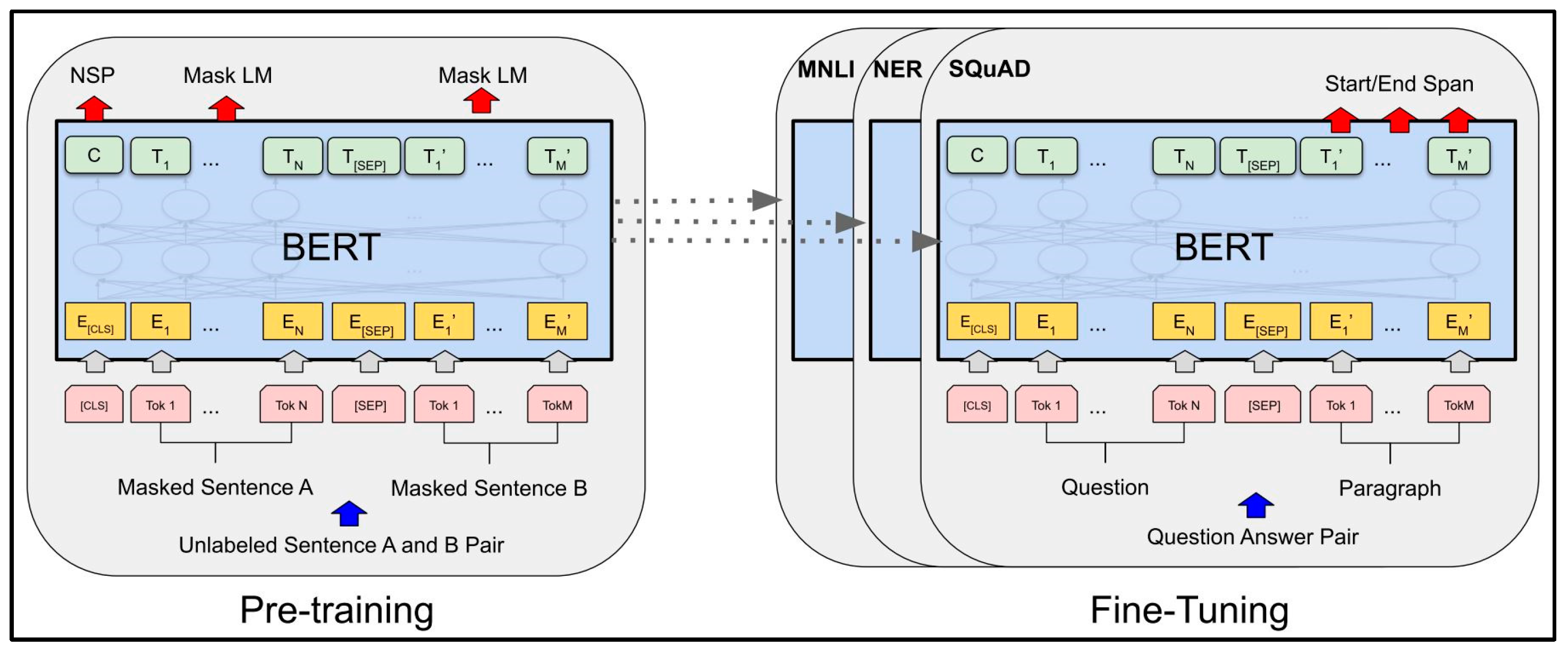
3.2. Bidirectional Encoder Representations from Transformers

The Bidirectional Encoder Representations from Transformers (BERT) is a language representation model introduced by Devlin et al. [47] at Google; it is a versatile tool that can be applied to a wide range of tasks such as language inference and question answering. Its architecture is founded on the original implementation described in [48]. Unlike the early versions of the Generative Pre-Training of Graph model (GPT) [49], BERT utilizes bidirectional self-attention, allowing each token to attend to both its preceding and subsequent context. Conversely, GPT utilizes unidirectional self-attention, enabling each token to attend solely to the context preceding it.

BERT employs a two-step process for executing a range of Natural Language Processing (NLP) tasks, which are pre-training and fine-tuning, illustrated in Figure 1. In the pre-training phase, the model is trained on an extensive text corpus to acquire a comprehensive understanding of language. The objective of pre-training is to create a model that can be fine-tuned for various downstream tasks, including text classification, question answering, and natural language generation. Fine-tuning refers to the process of training a pre-trained BERT model for a specific downstream NLP task.

During the pre-training phase, the BERT model is trained using a masked language modeling (MLM) task and a next sentence prediction (NSP) task. In the MLM task, a percentage of tokens in the input text are randomly masked, and the model is trained to predict the original token based on the context of the surrounding words. The NSP task involves providing two sentences as input and the model needs to predict whether the second sentence follows the first sentence in the original text. By training on these tasks, BERT learns to represent words and sentences in a way that captures their contextual meaning and relationships, which is important for many downstream NLP tasks. Once pre-trained, the BERT model can be fine-tuned on specific tasks with relatively small amounts of task-specific labeled data to achieve state-of-the-art performance [47].

Fine-tuning involves substituting the final layer of the pre-trained model with a task-specific layer, which is then trained on labeled data for the new task. This approach allows the BERT model to leverage its pre-training to acquire general language understanding and then use the fine-tuning step to adapt to the specificities of the new task [47]. For instance, if we are using BERT for text classification, we would replace the pre-training task’s final layer with a classification layer and fine-tune the model on the text classification task with labeled data. Likewise, if we aimed to apply BERT for a question-answering task, we would substitute the final layer with a question-answering layer and fine-tune the model with labeled data specific to that task. The primary advantage of fine-tuning is that it enables the BERT model to be utilized for a diverse range of NLP tasks without necessitating significant modifications to the architecture or training methodology. By fine-tuning the pre-trained model for a particular task, the model can attain state-of-the-art performance even with limited amounts of task-specific labeled data.

3.3. K-Nearest Neighbour Regression (kNN)

The K-Nearest Neighbor algorithm is a well-established machine learning technique, frequently employed for classification and regression tasks. Its primary objective is to classify unmarked data points by assigning them to the category of the nearest labeled data point [50]. The algorithm’s proficiency lies in its ability to leverage similarity metrics, which measure the distance between data points to identify the most analogous labeled data point. K-Nearest Neighbor Regression is a data-driven regression technique that does not rely on predefined parametric relationships between predictor and predicted variables. Instead, it utilizes information from observed data to make real-time predictions of the predicted variable. In regression tasks, K-Nearest Neighbor estimates the response of a test point (x_t) by taking a weighted average of the responses from the k closest training points (x(1), x(2), …, x(k)) in the vicinity of x_t. A kernel function is commonly employed to determine the weight assigned to each neighbor based on its proximity to the test point. Considering a training dataset X = {x₁, x₂, …, x_M} comprising M training points, each with N features, the weighted Euclidean distance can be utilized to measure the closeness between each training point x_i and the test point x_t [51,52]. Euclidean distance is measured according to Equation (7) [52].

$$D\left(x_t,x_i\right)=\sqrt{\sum _{n=1}^N{w}_n{(x_{t,n}-x_{i,n})}^2}$$

(7)

where N represents the number of features, x_t,n refers to the n^th feature value of the testing point x_t, and x_i,n represents the nth feature value of the training point x_i. The weight assigned to the nth feature is denoted as w_n, and it ranges between 0 and 1.

Next, kernel regression is applied and the estimation of response x_t is calculated according to Equation (8).

$$\widehat{f}(x_t)=\frac{\sum _{i=1}^k\varnothing \left(x_t,x_i\right)f\left(x_{\left(i\right)}\right)}{\sum _{i=1}^k\varnothing \left(x_t,x_i\right)}$$

(8)

where k represents the number of nearest neighbors employed for regression, ϕ(x_t, x_(i)) represents a kernel function centered at the i^th training point x_(i), and f(x_(i)) represents the known response of x_(i).

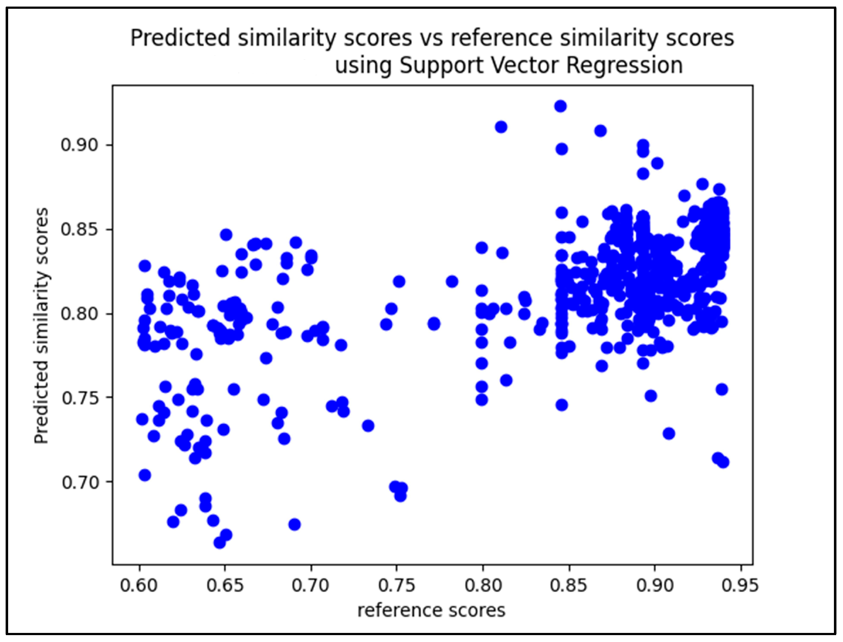
3.4. Support Vector Regression

Support Vector Regression (SVR) is a machine learning technique that is based on Vapnik–Chervonenkis (VC) theory, which has gained considerable attention due to its robustness and high accuracy. This method utilizes a variety of unique features, including the use of kernels, sparse solutions, and VC control of the margin, in addition to the number of support vectors [53]. One of the key characteristics of SVR is the introduction of an ε-insensitive region around the function, which is commonly referred to as the e-tube. The e-tube reformulates the optimization problem by identifying the tube that best approximates the continuous-valued function while balancing model complexity and prediction error. The optimization problem for SVR is formulated by first defining a convex e-insensitive loss function that needs to be minimized. The primary objective is to find the flattest tube that contains most of the training instances. This method achieves a high level of accuracy by striking a balance between the complexity of the model and the margin of error in the prediction [53].

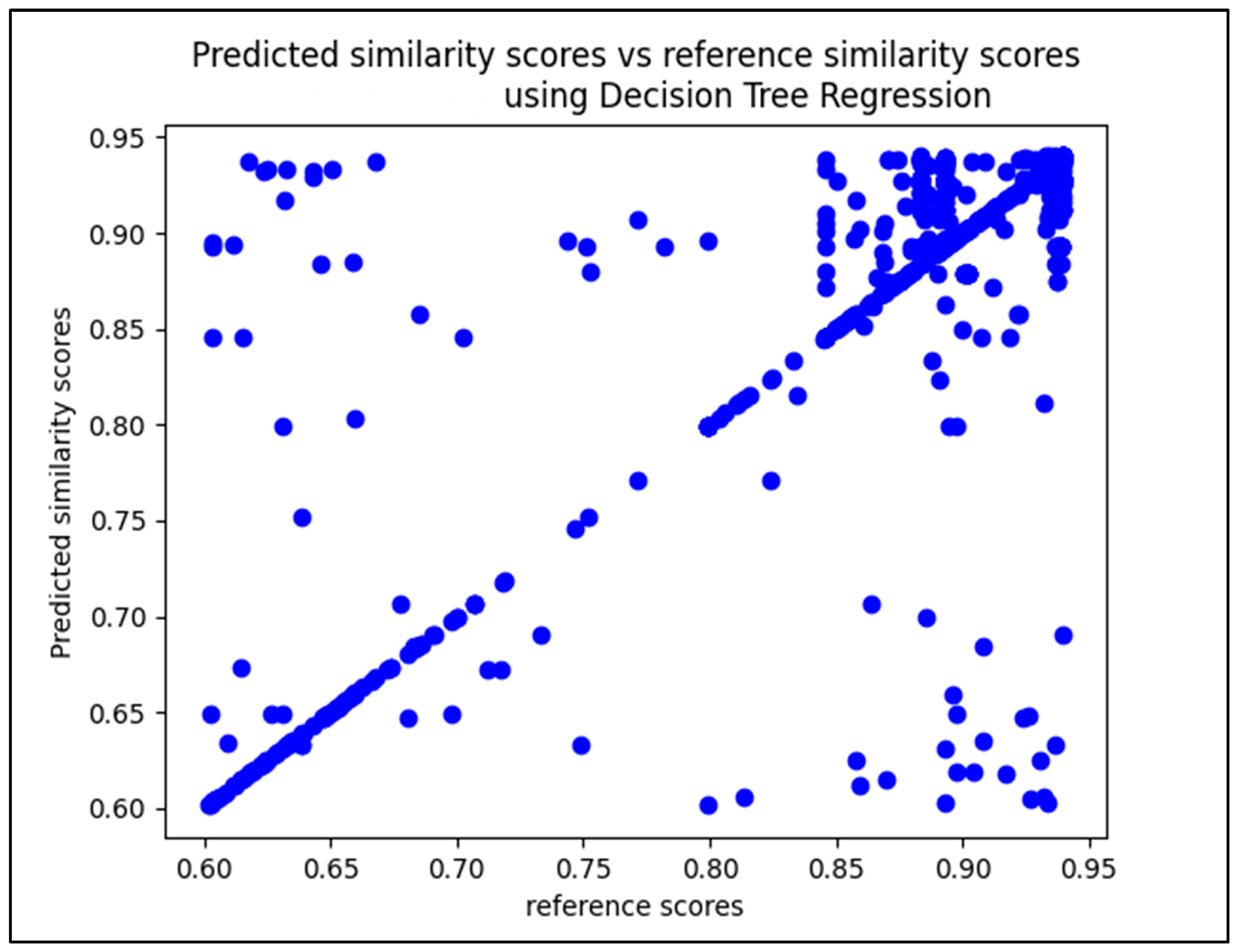
3.5. Decision Tree Regression

A Decision Tree is a data structure consisting of an arbitrary number of nodes and branches at each node, which is widely used in machine learning. Decision Tree Regression (DTR) employs a rapid divide-and-conquer greedy algorithm that recursively divides the data into smaller sections. This algorithm repeatedly selects the feature that maximizes the information gain and then partitions the data based on the selected feature, eventually creating a tree structure that provides a sequence of decision rules for prediction purposes [54]. The algorithmic process of the Decision Tree involves determining the predictive accuracy criteria, which can be achieved through various methods such as test sample error, cross-validation error, or re-substitution error. After defining the accuracy criteria, the next step involves selecting the optimal split based on the chosen criteria. Finally, the algorithm determines the stopping point for splitting and selects the optimal tree structure [55]. In the first step, the re-substitution error is computed using the same dataset that was utilized to build the predictor p. This error is calculated as the Mean Squared Error between the predicted values and the actual values of the dataset. To calculate the cross-validation error in Decision Tree regression, the dataset is partitioned into k subsets, referred to as “folds”. The model is then trained on k − 1 folds, while the remaining fold is used for testing. This process is repeated k times, with each fold serving as the test set once. The resulting k testing errors are averaged to compute the cross-validation error. By evaluating the model’s performance on multiple test sets, the cross-validation error provides a more reliable measure of the model’s ability to generalize to new data and prevent overfitting. The sample error is calculated by dividing the total number of cases into two subsamples, X₁ and X₂, with sizes of N₁ and N₂, respectively.

In the second step, the splits are selected, then evaluated based on the measure of node impurity. The most commonly used method for this is the Least-Squared Deviation, which is represented in Equation (9) [55].

$$R\left(t\right)=\frac{1}{N_w\left(t\right)}\sum _{i\in t}{w}_i{f}_i({u_i-\stackrel{-}{v}(t))}^2$$

(9)

where N_w is the weighted number of cases in node t, w_i is the value of weighting variable for case i, f_i represents the value of the frequency variable, u_i is the value of the response variable, and $\stackrel{-}{v}(t)$ is the weighted mean for node t.

In the last step, the determination of when to stop splitting takes place, and this relies on the minimum number of nodes. The selection of the right-sized tree (called the optimum tree) comes next, and it is obtained by using what is called tree pruning to reduce the risk of overfitting and improve the model’s generalization performance. Tree pruning involves removing branches or nodes from the tree that provide little or no additional information gain in the prediction of the target variable [55].

3.6. Evaluation Metrics

In this subsection, we present the metrics used for the evaluation of the fuzzy string-matching algorithms, BERT model, and the proposed hybrid method.

3.6.1. Confusion Matrix and Thresholds

The confusion matrix is a tool commonly used in machine learning to display statistical information on the predictions of a model compared to the actual classifications [55], which refers to the actual similarity score generated by benchmark. It reports four primary values: true positive (TP), true negative (TN), false positive (FP), and false negative (FN). TP represents the number of instances that the machine learning model correctly predicted as belonging to a specific class, which aligns with the actual results of the reference alignment. Conversely, TN indicates the number of instances that the model correctly predicted as not belonging to a specific class, in agreement with the actual reference alignment results. FP represents the number of instances that the model predicted as belonging to a particular class, but the reference alignment results indicate otherwise. FN indicate the number of instances that the model predicted as not belonging to a specific class, whereas the actual results of the reference alignment indicate the opposite.

In this study, we created confusion matrices to examine the performance of the proposed method at three thresholds of 0.70, 0.80, and 0.90. In the context of ontology alignment evaluation, a threshold refers to the optimal similarity score value that enables us to assess whether aligned ontologies are similar or not. A higher threshold value indicates a stricter evaluation criterion, leading to more dependable final outcomes. Conversely, a lower threshold value results in a more lenient evaluation criterion, leading to less trustworthy results.

3.6.2. Precision

Precision is a very popular method for evaluation of machine learning models. Its calculation is based on the concepts of TP and FP explained in the preceding subsection. In the context of ontology alignment, precision is defined as the ratio of the number of the correct alignments predicted by the proposed model as true positives to the total number of all correct alignments [56]. Precision is generally calculated according to Equation (10).

$$Precision=\frac{TP}{TP+FP}$$

(10)

Given R as the reference alignment, and A as the prediction of the alignment system (the proposed method), the precision of A is defined with Equation (11) [56]:

$$Precision(A)=\frac{|R\cap A|}{\left|A\right|}$$

(11)

where $|R\cap A|$ is the number of predictions that are correct matches according to the reference alignment, and $\left|A\right|$ is to total number of all pairs of classes of ontologies that are predicted as correct matches by the alignment system (proposed method).

3.6.3. Recall

Recall indicates how many instances are predicted positive out of all actually positive values. Recall is calculated by Equation (12).

$$Recall=\frac{TP}{TP+FN}$$

(12)

The same as with precision, given R as the reference alignment, and A as the predictions of the alignment system (our proposed method), the recall is calculated by Equation (13) [56]:

$$Recall(A)=\frac{|R\cap A|}{\left|R\right|}$$

(13)

where $|R\cap A|$ is the number of predictions correctly made by the alignment system (the proposed method) that match the reference alignment, and $\left|R\right|$ is the cardinality of matched pairs of the aligned classes in the reference alignment.

3.6.4. F1-Score

F1-score, also called F-measure, is the harmonic mean between precision and recall [56]. It is given by Equation (14).

$$F1-score=2\ast \frac{precision\times recall}{precision+recall}$$

(14)

Specifically, the F1-score with reference to ontology alignment is given by Equation (15) [56].

$$f-measure(A)=\frac{recall\left(A\right)\mathrm{x} precision\left(A\right)}{\alpha \mathrm{x} recall\left(A\right)+\left(1-\alpha \right)\mathrm{x} precision\left(A\right)}$$

(15)

In this study, the relative weight of recall and precision, denoted by α, has been set to 0.5. This default weight is usually set to 0.5 which gives the same value when the F-measure is calculated using Equation (12). In some cases, weight can be higher for recall and lower for precision. In such cases, one can determine the value of the weight for the recall by applying Equation (13). The weight must be a decimal value in the range 0 and 1.

3.6.5. Accuracy

Accuracy is a critical performance metric in machine learning, which measures the extent to which a model’s output matches the intended or desired outcome. In this context, accuracy is typically assessed by comparing the predicted outputs of a model to a set of known or labeled data points. The effectiveness of a model’s accuracy is often evaluated based on the level of user effort required to transform the machine-generated results into the intended outputs [57]. Achieving high accuracy in machine learning is essential for ensuring the model’s reliability and usability, as it directly impacts its ability to generalize and make accurate predictions on new, unseen data. Accuracy is the percentage of the correct predictions made by the machine learning model. It is simply calculated by summing TP and TN divided by total number of rows in the dataset.

3.6.6. Mean Square Error (MSE) and Root Mean Square Error (RMSE)

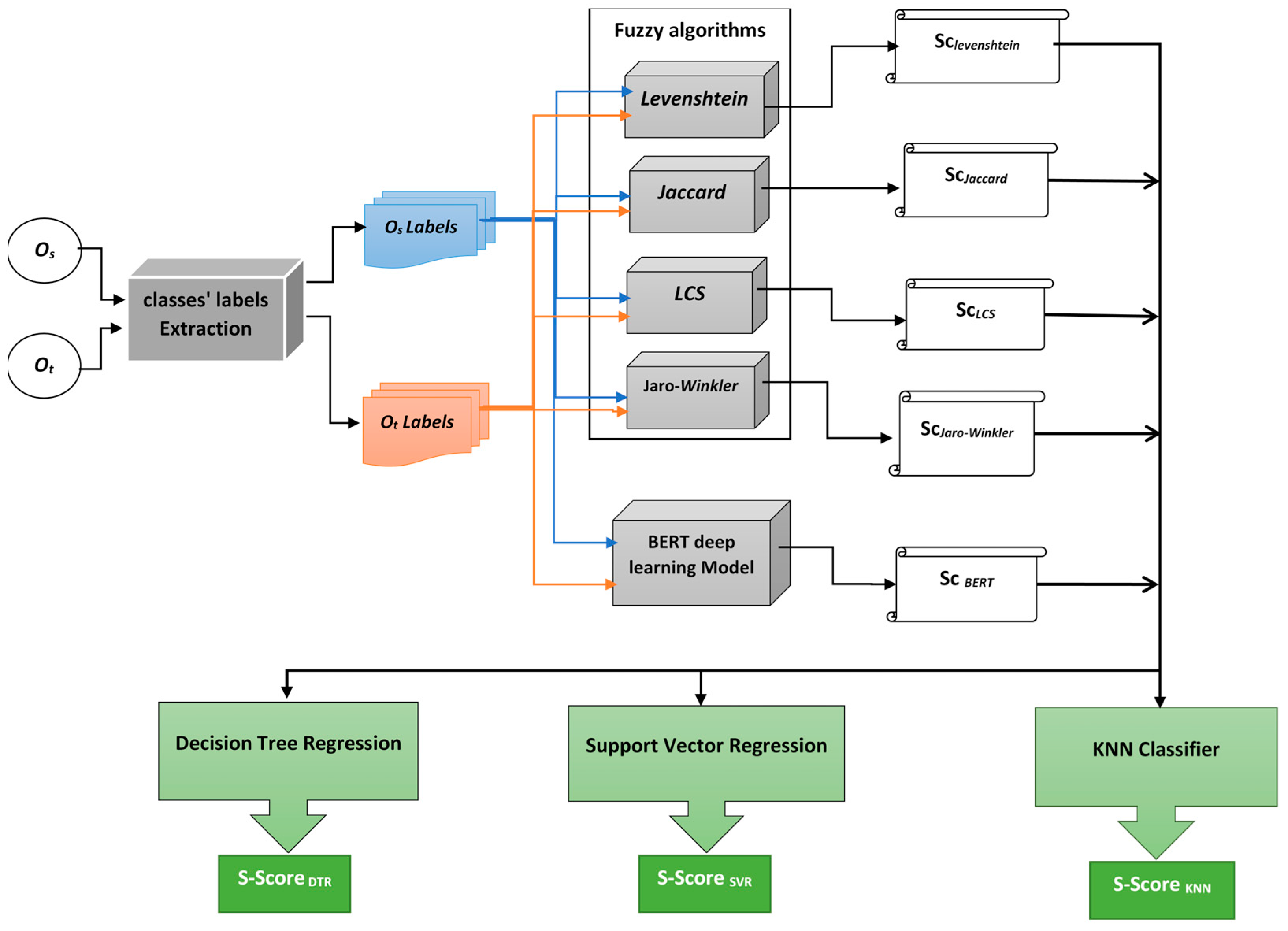
The Mean Squared Error (MSE) is a widely used performance metric that quantifies the average discrepancy between the observed values and the model’s predicted values. MSE is calculated by taking the average of the squared differences between the predicted and observed values, providing a measure of the model’s overall accuracy. This metric is particularly useful for assessing the effectiveness of regression models, where the goal is to minimize the error between the predicted and actual values.

The Root Mean Squared Error (RMSE) on the other hand is a widely used performance metric in machine learning that measures the average magnitude of the errors between the predicted and observed values. RMSE is a valuable tool for evaluating the accuracy of a predictive model after the algorithm has converged. This metric is also especially useful in regression tasks where the goal is to minimize the error between the predicted and actual values, and it provides a measure of the model’s predictive ability [58]. RMSE is calculated by Equation (16) [58].

$$RMSE=\sqrt{\frac{1}{m}\sum _{i=1}^m{(e_i-{\tilde{e}}_i)}^2}$$

(16)

where e_i and ${\tilde{e}}_i$ represent the original and estimated attribute values, respectively, and m is the total number of predictions. A larger RMSE value indicates a less accurate model, whereas a smaller RMSE value indicates a higher degree of predictive accuracy.

4. Proposed Method

Our proposed method employs a suite of fuzzy string-matching algorithms to facilitate the alignment of ontologies at the lexical level. Specifically, we utilized the Jaccard, Jaro–Winkler, Levenshtein, and LCS algorithms, which have been extensively validated in the literature for their effectiveness in this context. While the Word2Vec algorithm has shown promise in some applications, we found it to be unsuitable due to its inability to handle strings with multiple tokens, as attested by Rudwan et al. [20]. In addition to these lexical matching algorithms, we incorporate BERT, a powerful language model that leverages contextual information to tackle the semantic aspect of ontology alignment. To combine the similarity scores obtained from these algorithms, we use three regression classifiers as depicted in Figure 2. This enables us to fully leverage the strengths of each algorithm while mitigating their weaknesses, resulting in a more accurate and comprehensive alignment of ontologies.

Figure 2 displays the workflow of our proposed method for ontologies alignment using a combination of lexical and semantic similarity metrics. The method begins by extracting labels from the source and target ontologies (O_s and O_t), resulting in two sets of labels, O_s Labels and O_t Labels, respectively. Next, we apply a suite of fuzzy string-matching algorithms recursively to align each pair of labels in the two sets. For each fuzzy string-matching algorithm, the similarity scores are computed and stored in a separate text document. This produces a set of similarity scores for each pair of aligned labels, that capture the lexical similarity between them. To incorporate semantic information into the alignment process, we use BERT version 2.2.2 available in the “sentence-transformers” Python library package to compute the semantic similarity scores between every pair of aligned labels in O_s Labels and O_t Labels. These scores are stored in a separate text document, SC_BERT, which captures the semantic similarity between the aligned labels. Finally, we combine the lexical and semantic similarity scores using three regression classifiers, namely, kNN, SVR, and DTR. Each classifier produces a final similarity score for each pair of aligned labels, which summarizes the overall similarity score considering both the lexical and semantic features of the input ontologies O_s and O_t. Algorithm 1 presents a detailed breakdown of the implementation of the proposed method shown in Figure 2.

Table 1. Variables used in Algorithm 1.

Variable Name	Description
Os	Source ontology
Ot	Target ontology
reference	An xml document containing the similarity scores between each pair of classes in Os and Ot
osLabels	A document containing the labels of all classes in the source ontology
otLabels	A document containing the labels of all classes in the target ontology
finalScores	A csv document containing the similarity scores for both fuzzy string-matching algorithms and BERT
refAMLFile	A csv documents containing three columns representing the URIs of each pair of classes from Os and Ot and their similarity scores generated by the baseline AML alignment system
smKNNScores	A csv document containing the final similarity scores of the alignment by the SM-kNN model
smSVRScores	A csv document containing the final similarity scores of the alignment by the SM-SVR model
smDTRScores	A csv document containing the final similarity scores of the alignment by the SM-DTR model

provides a summary of the variables used in Algorithm 1 and their respective descriptions.

To evaluate the effectiveness of our proposed method, we compared it to the widely-used AML system [31] version 3.2 as a baseline for aligning two ontologies. In this experiment, we set the AML threshold to 0.60 and used the mouse and human ontologies as the source ontology (O_s) and target ontology (O_t), respectively. These ontologies were downloaded from the anatomy track in the OAEI 2022. To evaluate the performance of our proposed method against the widely-used AML alignment system, we first fed AML with the source ontology and target ontology to obtain the reference similarity scores in line 3 of Algorithm 1. The GetURIsScores() function then takes the reference as a parameter to extract the URIs of each pair of matched classes, as well as their similarity scores, and store this information in the refAMLFile file in line 4. In lines 6–17 of Algorithm 1, the classes’ URIs are read from the refAMLFile file and passed to a SPARQL query to extract their labels; the extracted classes’ labels are then stored in osLabels and otLabels files for the source and target ontologies, respectively. The fuzzy string-matching algorithms are then applied for lexical alignment, followed by BERT for semantic alignment, in lines 19–25. The similarity scores obtained by each algorithm are stored in the finalScores file in line 26. Next, in lines 28–30 of Algorithm 1, the reference similarity scores obtained by the AML system are appended to the finalScores file to prepare the data for the training of the models. The dot product in line 29 of Algorithm 1 indicates that the resulting values will be stored in the finalScore CSV file. This is followed by the training of the SM-kNN, SM-SVR, and SM-DTR models in lines 32–34 of the algorithm. Finally, the trained SMKnnModel, SMSvrModel, and SMDtrModel models are used to predict the similarity scores for each pair of classes in the input ontologies O_s and O_t in lines 36–38. The predicted similarity scores for each model are then stored in a CSV file with three columns for the source class, the target class, and the predicted similarity score (lines 36–38). The next section presents and discusses the experimental results of the study.

Algorithm 1: Hybridizing fuzzy string matching and BERT using regression classifiers

Inputs: Os, Ot, reference Outputs: smKNNScores, smSVRScores, smDTRScores, finalScores reference ← AML_alignment(Os, Ot) refAMLFile ← GetURIsScores(reference)   For each row in refAMLfile Do   uriSource ← ReadUri(row(1))   uriTarget ← ReadUri(row(2))   osLabels ← SPARQL(     “SELECT DISTINCT? label     WHERE { <“+uriSource+”> rdfs:label? label}”     )    otLables ← SPARQL(     “SELECT DISTINCT ?label     WHERE { <“+uriTarget+”> rdfs:label ?label }”     ) EndFor   For each sourceElem, targetElem in oslabels, otlabels Do    scLev ← Levenshtein(sourceElem, targetElem)    scLcs ← LCS(sourceElem, targetElem)    scJaccard ← Jaccard(sourceElem, targetElem)    scJaro ← JaroWinkler(sourceElem, targetElem)    scBert ← BERT(sourceElem, targetElem) EndFor finalScores.AddRow(scBert, scJaro, scLev, scLcs, scJaccard)   For each score, row in refAMLFile, finalScores Do    finalScores.AddColumn(row, score) EndFor   SMKnnModel ← SM-KNNTraining(finalScores) SMSvrModel ← SM-SVRTraining(finalScores) SMDtrModel ← SM-DTRTraining(finalScores)   smKNNScores ← getScorePredictions(SMKnnModel, finalScores) smSVRScores ← getScorePredictions(SMSvrModel, finalScores) smDTRScores ← getScorePredictions(SMDtrModel, finalScores)

5. Experimental Results and Discussion

As explained in Algorithm 1, the AML alignment system was used as the baseline for generating the reference similarity scores, for training the classifiers in the proposed method. Furthermore, the reference alignment provided in OAEI 2022 prescribed a similarity score of 1.0 for each pair of aligned classes. By setting the threshold to 0.60 in the AML system, we were able to obtain 1400 pairs of similar classes from the mouse and human ontologies. Three different thresholds, 0.70, 0.80, and 0.90, were used to evaluate the performance of the algorithms in the proposed method. In the following subsections, we present the similarity scores obtained by the fuzzy string-matching algorithms and BERT. This is followed by an analysis of the performance of these algorithms, in terms of precision, recall, F1-score, and accuracy. Finally, the performance of the proposed method is evaluated by analyzing the performance of the three hybrid models of the proposed method, namely, SM-kNN, SM-SVR, and SM-DTR, using the precision, recall, F1-score, and accuracy, as well as the running time, MSE, and RMSE.

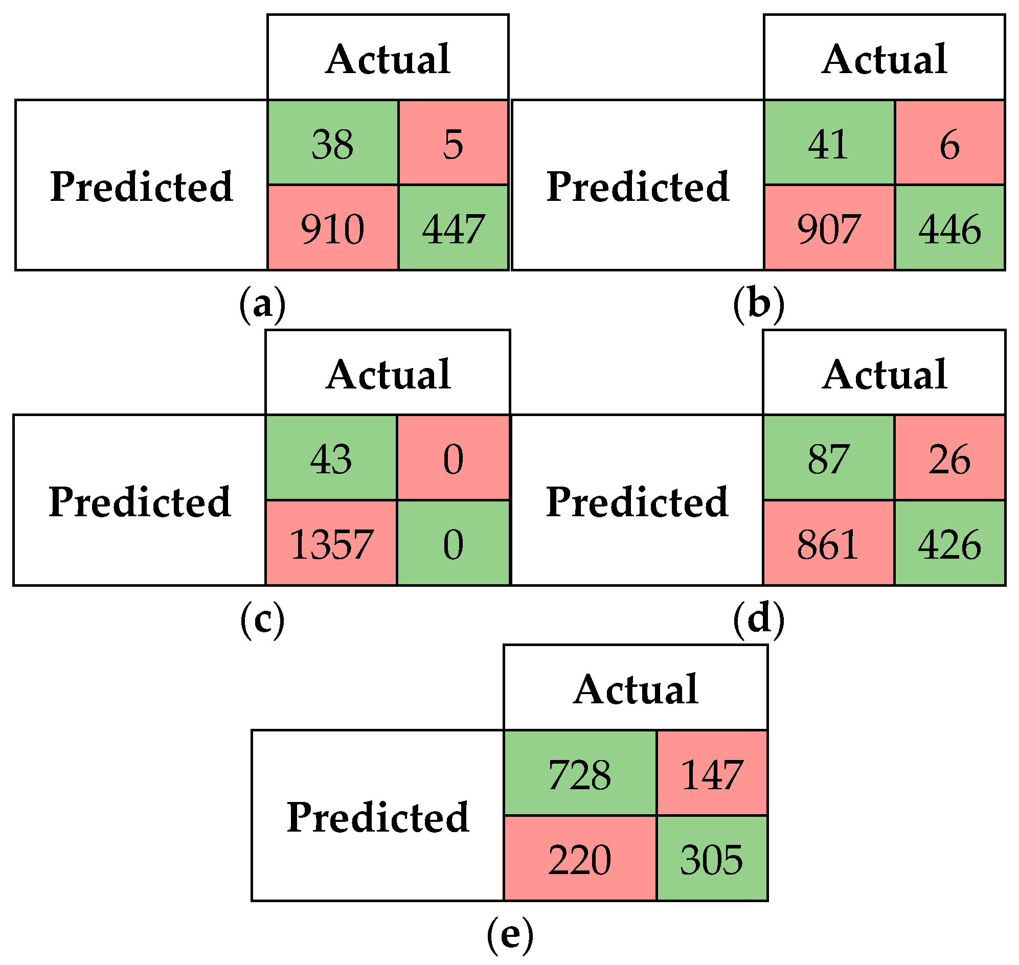
5.1. Performancee Evaluation of Fuzzy String-Matching Algorithms and BERT

Table 2. Top similarity scores obtained by the algorithms.

Algorithm	Sc1	Sc2	Sc3	Sc4	Sc5	Sc6	Sc7	Sc8	Sc9	Sc10
Levenshtein	0.941176471	0.9375	0.933333333	0.933333333	0.933333333	0.928571429	0.928571429	0.928571429	0.928571429	0.928571429
LCS	0.941176471	0.9375	0.933333333	0.933333333	0.933333333	0.928571429	0.928571429	0.928571429	0.928571429	0.928571429
Jaccard	0.94	0.94	0.93	0.93	0.93	0.93	0.93	0.93	0.93	0.93
Jaro–Winkler	0.960784314	0.955555556	0.955555556	0.955555556	0.952380952	0.952380952	0.952380952	0.948717949	0.948717949	0.944444444
BERT	1.0000004	1.0000002	1.0000002	1.0000002	1.0000002	1.0000002	1.0000002	1.0000002	1.0000002	1.0000002
AML System	0.94	0.94	0.94	0.94	0.94	0.94	0.94	0.94	0.94	0.94

provides the top 10 best similarity scores for the fuzzy string-matching algorithm, the BERT deep learning model, as well as the similarity scores obtained by the AML reference system. The scores are ranked from the highest (Sc1) to the lowest (Sc10). It can be seen that the Jaro–Winkler algorithm achieved the highest similarity score compared to the other fuzzy algorithms. In contrast, BERT recorded the best similarity score of 1.0, indicating close semantic relations between the input ontologies.

Table 2 further indicates that the Jaccard, Levenshtein, and LCS fuzzy string-matching algorithms yielded equivalent similarity scores to the baseline’s performance of 0.94 for some pair of classes in the input ontologies. However, the Jaro–Winkler algorithm performed better than the baseline score, achieving a higher similarity score of 0.96 for some pair of classes in the input ontologies. Furthermore, although the remaining scores for Levenshtein, LCS, and Jaccard algorithms are slightly lower than the baseline’s performance of 0.94, the Jaro–Winkler algorithm achieved better similarity scores than the baseline for the remaining scores in Table 2. In contrast, BERT demonstrated consistent and superior performance across all similarity scores, outperforming the fuzzy string-matching algorithms. The top similarity score obtained by BERT was the same for the remaining scores, but with higher scores than the other algorithms, including the baseline AML system. These results highlight the effectiveness of BERT in achieving high similarity scores, indicating its potential for improving ontology alignment.

The performance of the fuzzy string-matching algorithms and BERT was further evaluated in terms of precision, recall, and F1-score. The confusion matrices for all the algorithms are given in Figure 3 for a threshold of 0.70. From the confusion matrices, it is evident that BERT outperformed the fuzzy string-matching algorithms with the highest number of true positives at 1247. Among the fuzzy string-matching algorithms, Jaro–Winkler had the best performance in terms of true positives. Once again, the confusion matrices indicate the potential of BERT in ontology alignment.

Table 3. Performance of fuzzy string-matching algorithms and BERT at threshold 0.70.

Variable Name	LCS	Levenshtein	Jaccard	Jaro–Winkler	BERT
Precision	0.969756098	0.986942329	1	0.965022422	0.927827381
Recall	0.766975309	0.699845679	0.697857143	0.830246914	0.96219
F1-score	0.856527359	0.818961625	0.822044594	0.892575695	0.94469697
Accuracy	76.2142857	71.3571429	69.7857143	81.5	89.5714286

presents the performance of each algorithm at threshold 0.70, in terms of precision, recall, F1-score, and accuracy. It is shown that the Jaccard algorithm achieved the highest precision of 1.0, followed by Levenshtein, LCS, Jaro–Winkler, and BERT, with precision scores of 0.987, 0.970, 0.965, and 0.928, respectively. On the other hand, BERT achieved the highest recall score of 0.962, outperforming the other algorithms. BERT also recorded the highest F1-score compared to the fuzzy string-matching algorithms. In terms of accuracy, BERT obtained the highest accuracy of 89.6%, outperforming all fuzzy string-matching algorithms, and followed by the Jaro–Winkler algorithm as the second-best with 81.5% accuracy. Jaccard had the lowest accuracy score of 69.8%. Overall, at the threshold of 0.70, BERT outperformed the fuzzy string-matching algorithms in ontology alignment. Among the fuzzy string-matching algorithms, Jaro–Winkler consistently performed better than LCS, Levenshtein, and Jaccard. The threshold was increased to 0.80 to obtain the confusion matrixes in Figure 4 for the fuzzy string-matching algorithms and BERT deep learning model.

Table 4. Performance of fuzzy string-matching algorithms and BERT at threshold 0.80.

Variable Name	LCS	Levenshtein	Jaccard	Jaro–Winkler	BERT
Precision	0.975425331	1	1	0.988250653	0.917348609
Recall	0.406619385	0.365642238	0.337142857	0.596532703	0.88337
F1-score	0.573971079	0.535487594	0.504273504	0.743980344	0.90004014
Accuracy	45.2857143%	42.5%	33.7142857%	62.7857143%	82.2142857%

displays the performance of the fuzzy string-matching algorithms and BERT deep learning model at threshold 0.80. The increasing of threshold to 0.80 resulted in a significant drop in recall for all fuzzy string-matching algorithms, with only slight improvements in precision. As shown in Table 4, the Jaro–Winkler algorithm remained the best-performing algorithm, achieving an F1-score of 0.744 and an accuracy of 62.8%. Despite underperforming in precision compared to the fuzzy string-matching algorithms, BERT outperformed the algorithms in terms of recall and F1-score, with values of 0.883 and 0.900, respectively. BERT also achieved the highest accuracy of 82.21%, compared to the fuzzy string-matching algorithms, followed by the Jaro–Winkler algorithm with 62.78% accuracy which outperformed the rest of fuzzy string-matching algorithms. To further challenge the algorithms, we raised the threshold to 0.90. Figure 5 displays the confusion matrices for the fuzzy string-matching algorithms and BERT at this threshold 0.90.

It can be observed in Figure 5 that the fuzzy string-matching algorithms detected very few true positives, while false negatives were more prevalent. Among the fuzzy string-matching algorithms, Jaro–Winkler performed the best in terms of true positives, detecting 87 cases, whereas Levenshtein performed the worst, detecting only 38 true positives. False positive cases were also relatively low and could be treated as true positives since the reference alignment provided by OAEI 2022 indicates that the similarity scores for all aligned pairs of classes should be 1.0.

In contrast, BERT outperformed all the fuzzy string-matching algorithms, detecting over 50% of the total alignments (i.e., 728 true positive cases).

Table 5. Performance of fuzzy string-matching algorithms and BERT at threshold 0.90.

Variable Name	LCS	Levenshtein	Jaccard	Jaro–Winkler	BERT
Precision	0.872340426	0.88372093	1	0.769911504	0.832
Recall	0.043248945	0.040084388	0.030714286	0.091772152	0.76793
F1-score	0.08241206	0.076690212	0.05959806	0.16399623	0.79868349
Accuracy	34.7857143%	34.6428571%	3.0714286%	36.6428571%	73.7857143%

summarizes the performance of the fuzzy string-matching algorithms and BERT in terms of precision, recall, F1-score, and accuracy at threshold 0.90. It is shown in Table 5 that the Jaccard algorithm achieved the highest precision, while the other fuzzy string-matching algorithms obtained lower precision scores compared to the previous thresholds of 0.70 and 0.80. However, in terms of recall, all fuzzy string-matching algorithms recorded lowest values, while BERT outperformed them, not only in terms of recall, but also in terms of precision, F1-score, and accuracy. Among the fuzzy string-matching algorithms, Jaro–Winkler had the highest accuracy score of 36.7%, while Jaccard achieved the lowest accuracy of 3.07%. The low accuracies indicate that fuzzy string-matching algorithms are not reliable at higher thresholds.

On the other hand, BERT was generally stable and reliable despite the decrease in its accuracy to 73.8% at threshold 0.90 compared to 82.2% and 89.6% at thresholds 0.80 and 0.70, respectively. This demonstrates that BERT outperforms fuzzy string-matching algorithms at different threshold due to its ability to handle the semantic features of the input ontologies. Therefore, it can be concluded that while fuzzy string-matching algorithms can be useful for lexical alignment at low thresholds, they are not reliable for comprehensive ontology alignment. BERT, on the other hand, has proven to be a more powerful tool for ontology alignment. The following subsection presents the results of our proposed method for hybridizing the similarity scores of fuzzy string-matching algorithms and the BERT deep learning model by the kNN, SVR, and DTR classifiers for improved ontology alignment. As indicated earlier, the use of the three classifiers to hybridize the fuzzy string-matching algorithms and the BERT model in the proposed method resulted into three hybrid models, namely, SM-kNN, SM-SVR, and SM-DTR. Therefore, here and after, the performance of the proposed method (Figure 2) is discussed in terms of its three hybrid models, SM-kNN, SM-SVR, and SM-DTR.

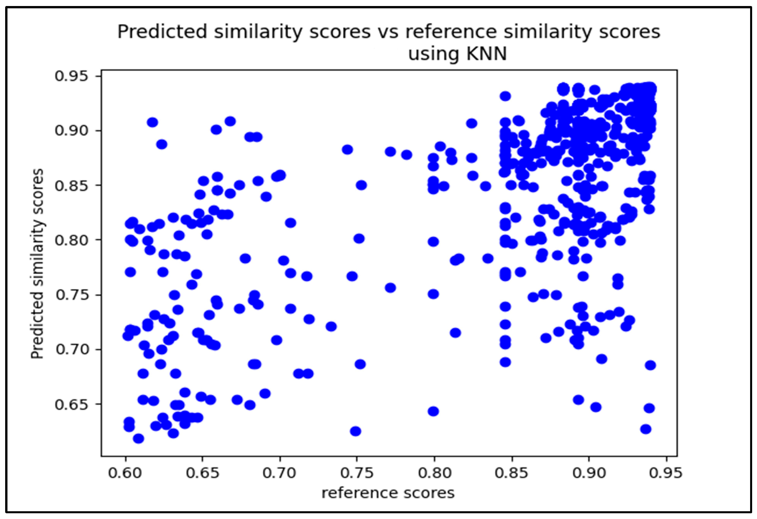
5.2. Performance of SM-kNN, SM-SVR, and SM-DTR Models

Let us recall that the aim of this study was to hybridize/combine the strengths of fuzzy string-matching algorithms and the BERT deep learning model to develop a method that considers both the lexical and semantic features of ontologies in the alignment process. By combining the strengths of both fuzzy string-matching algorithms and BERT, we sought to improve the accuracy and comprehensiveness of the alignment process. To this end, the similarity scores of the fuzzy string-matching algorithms and the BERT model (see part in Table 2) were further combined with three machine learning regression classifiers, namely, kNN, SVR, and DTR. To evaluate the performance of our proposed method, its three hybrid models, named SM-kNN, SM-SVR, and SM-DTR, were trained using the similarity scores obtained by the fuzzy string-matching algorithms and BERT for each pair of classes in the dataset, as well as the reference similarity scores obtained by the AML system. The following subsections discuss the performance of the three hybrid models (SM-kNN, SM-SVR, and SM-DTR) of the proposed method, in terms of precision, recall, F1-score, and accuracy at thresholds 0.70, 0.80, and 0.90, as well as error rates and running times.

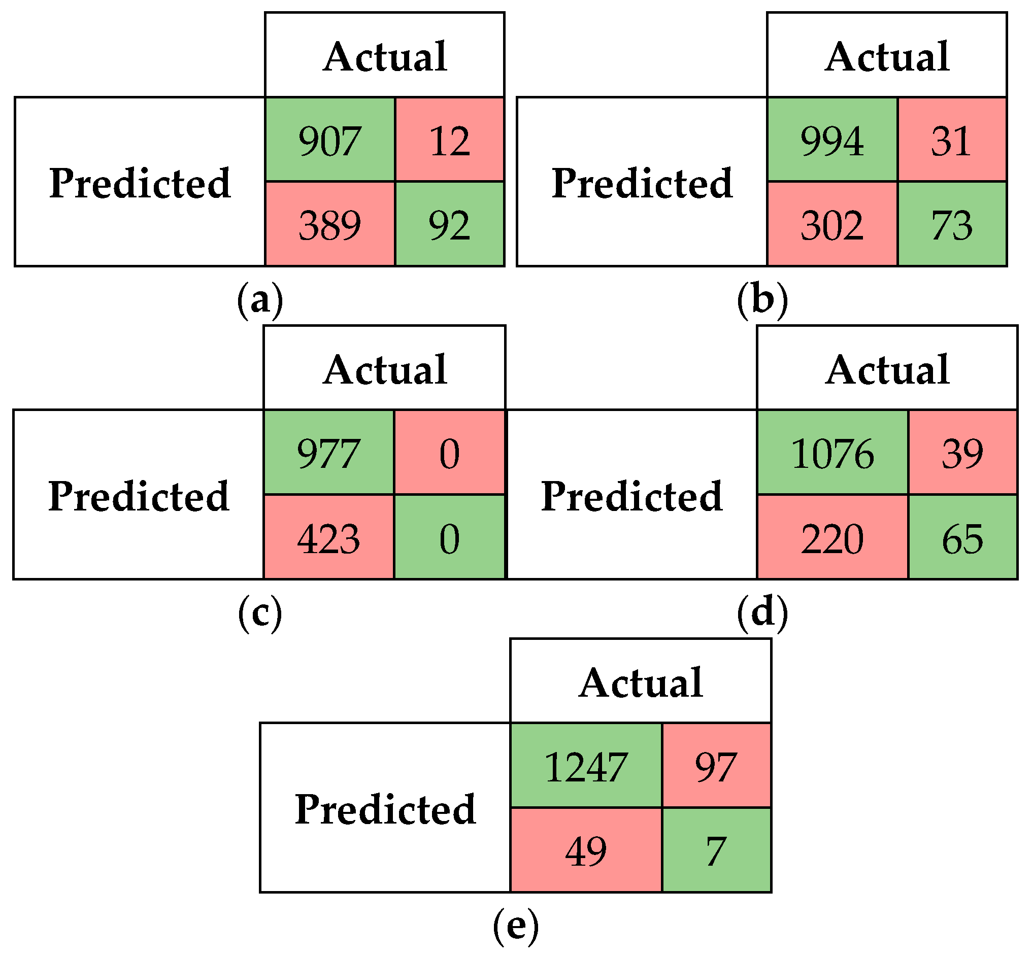
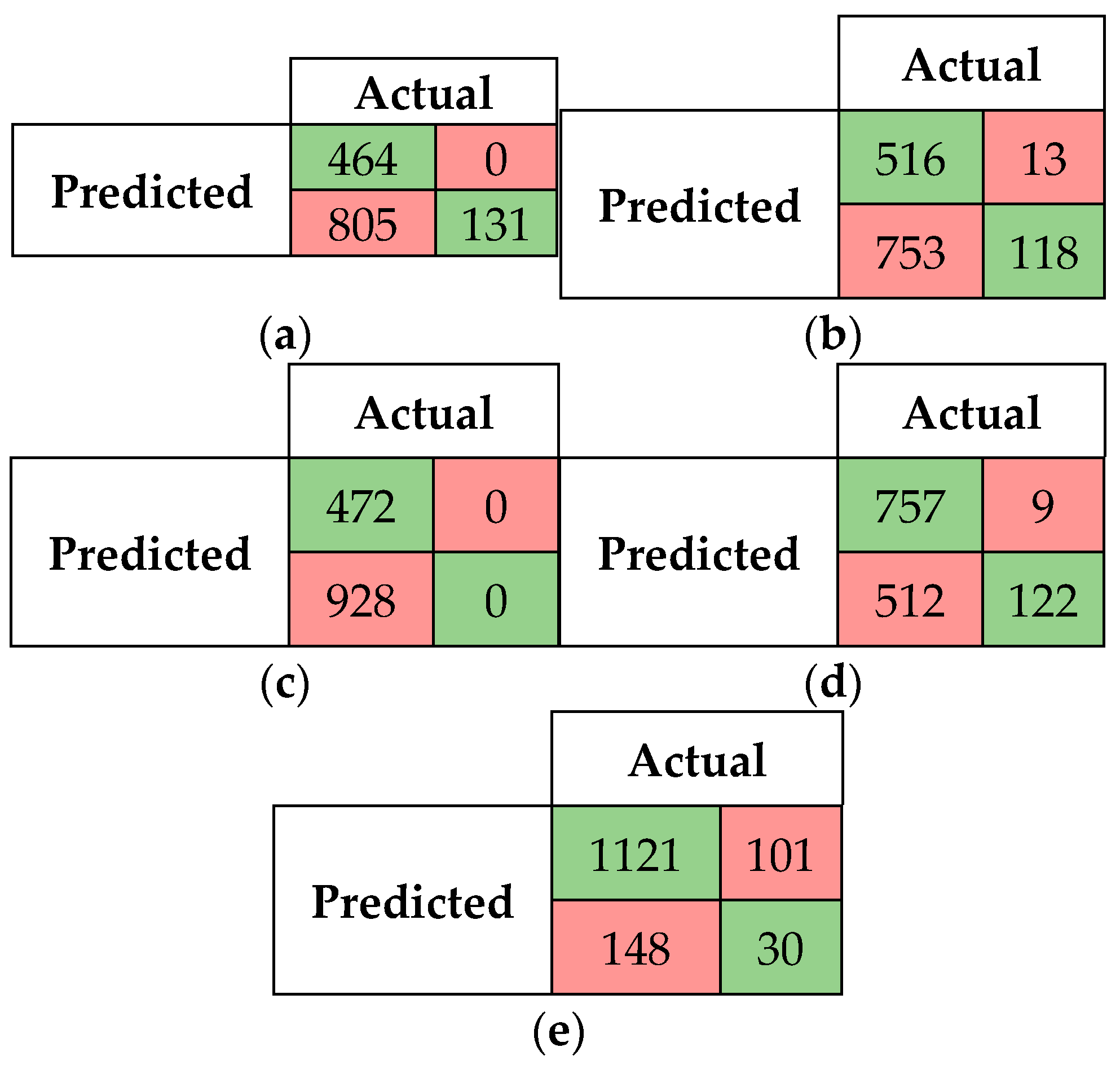
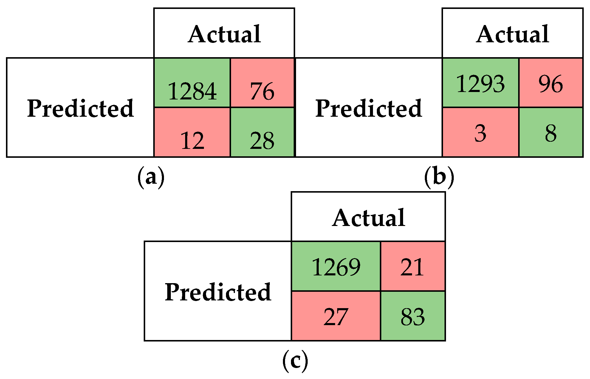
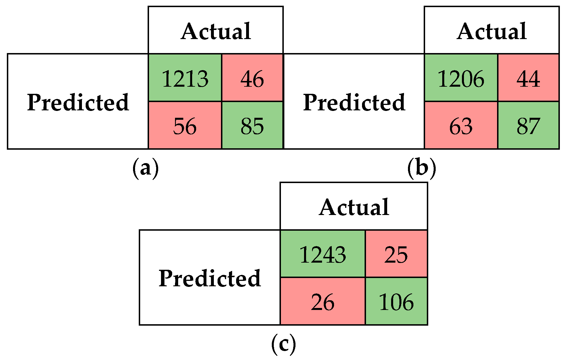
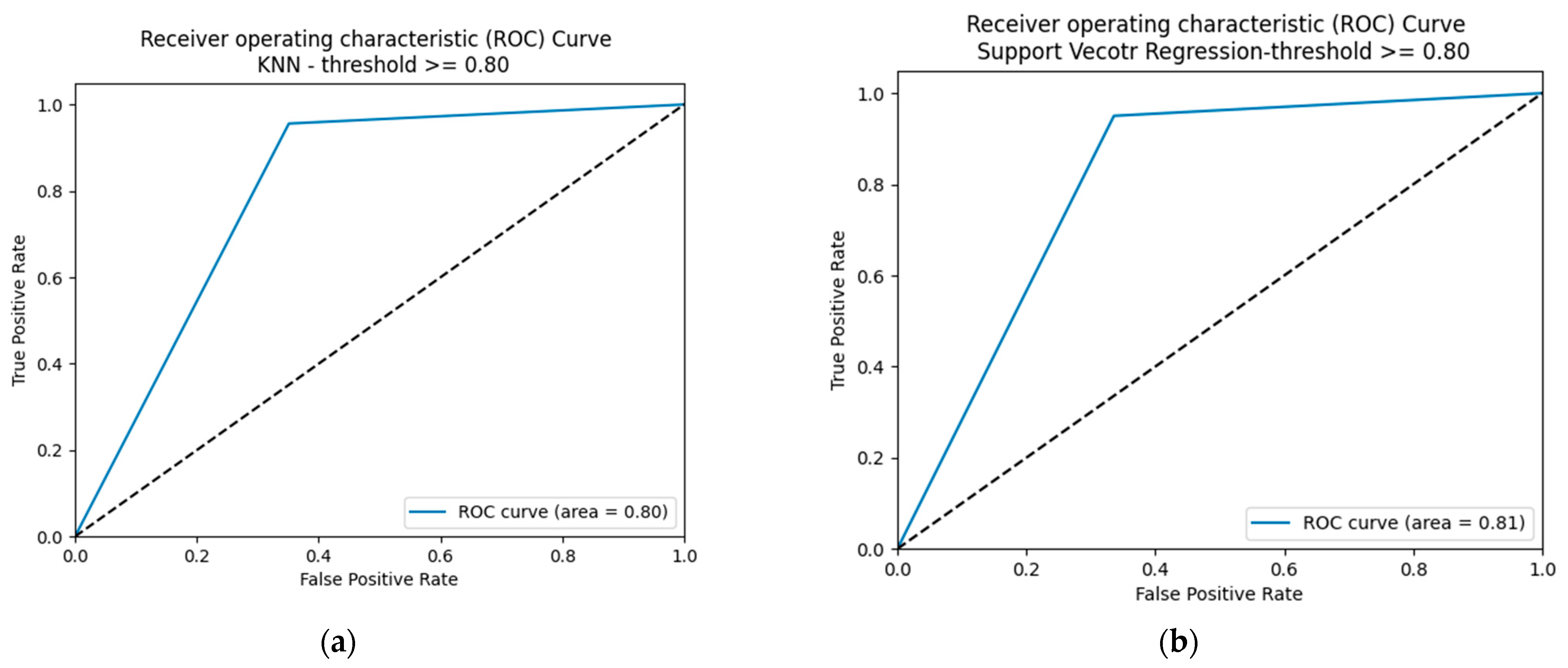
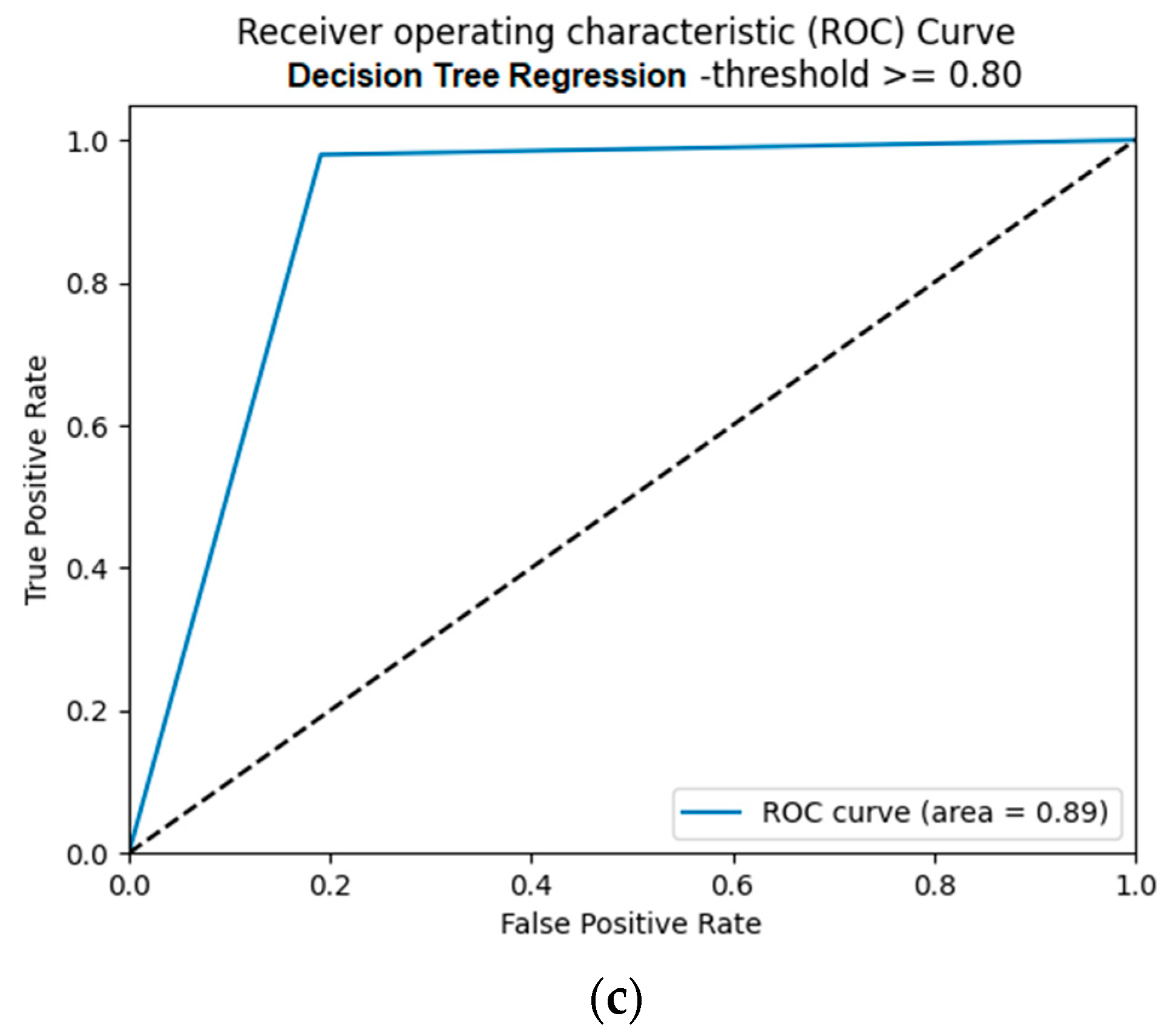
5.2.1. Confusion Matrices and Visual Presentation of the Proposed Model’s Performance

Figure 6, Figure 7 and Figure 8 present the confusion matrices for the SM-kNN, SM-SVR, and SM-DTR models at thresholds 0.70, 0.80, and 0.90, respectively. It can be seen in Figure 6 that the three models performed almost the same in terms of the number of true positive cases they predicted. However, the SM-SVR model outperformed the others by predicting 1293 true positive cases, while the SM-DTR model detected the least number of true positives with 1269. Comparing the number of true positive cases predicted by the three models to those of fuzzy string-matching algorithms and BERT (Figure 3, Figure 4 and Figure 5), one can see that the three hybrid models (SM-kNN, SM-SVR, and SM-DTR) of the proposed method based on kNN, SVR, and DTR classifiers outperformed the fuzzy string-matching algorithms and BERT. This indicates the effectiveness of the proposed method that harnesses the strengths of both the fuzzy string-matching algorithms and the BERT model for improved ontology alignment.

Figure 7 and Figure 8a–c presents the confusion matrixes for the SM-kNN, SM-SVR, and SM-DTR models at threshold 0.80 and 0.90. At threshold 0.80, the SM-DTR model outperformed the SM-kNN and SM-SVR models, with a higher number of true positives of 1243 cases predicated, followed by the SM-kNN model with 1213 true positives, and SM-SVR with 1206 true positives. The SM-DTR model also achieved a better performance at threshold 0.90 compared to other models with 893 true positives, followed by the SM-kNN model with 847 true positives. The SM-SVR model achieved the worst performance at threshold 0.90 with 0 true positives. These results further indicate that the combination of the strengths of fuzzy string-matching algorithms and the BERT model with machine learning regression classifiers led to better performance compared to using them individually (see Figure 3, Figure 4 and Figure 5). Figure 9, Figure 10 and Figure 11 present the scatterplot diagrams for the three models. These diagrams provide a visual representation of the distribution of similarity scores obtained by each model versus the reference scores obtained by the AML baseline system.

It is shown in Figure 9 that the majority of the plots are located in the top right corner, indicating that most of the similarity scores are higher. The few plots located in the right bottom area represent the false negatives. However, the left area of the diagram shows a mix of false positives and false negatives, as well as a limited number of true negatives. Nevertheless, the rate of false negatives located at the bottom area of the diagram is relatively less than the false positives that are located at the upper left area.

In the scatterplot diagram for the SM-SVR model in Figure 10 the majority of plots are clustered around the center-right of the diagram, with similarity scores ranging from 0.77 to 0.86. However, a few plots appear beyond 0.90, indicating performance close to that of the AML reference scores. Figure 11 displays the scatterplot diagram for the SM-DTR model. It appears that a large number of plots form a line with a 45-degree inclination angle, indicating that the majority of predictions made by the SM-DTR model are true positives. Furthermore, a significant number of plots are situated in the upper right corner of the diagram, demonstrating the ability of the SM-DTR model to accurately predict similarity scores with highest values between classes.

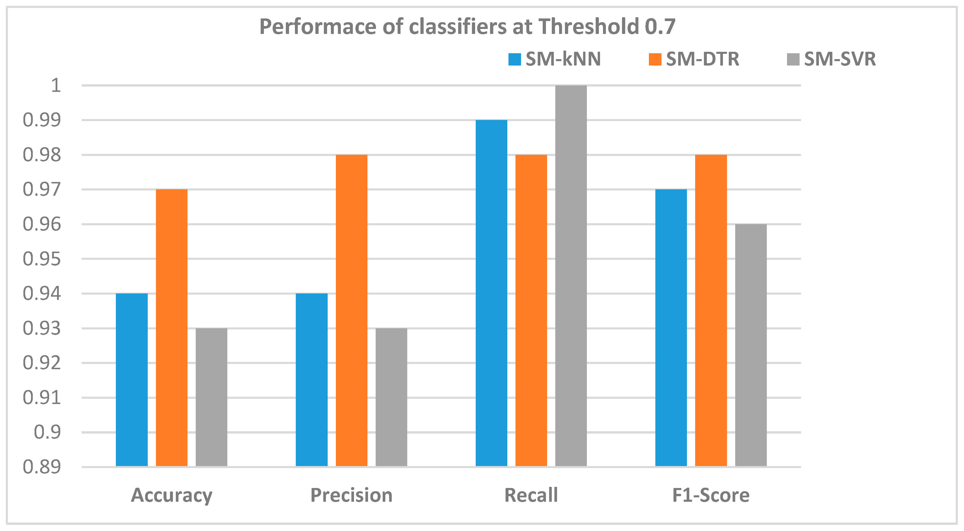
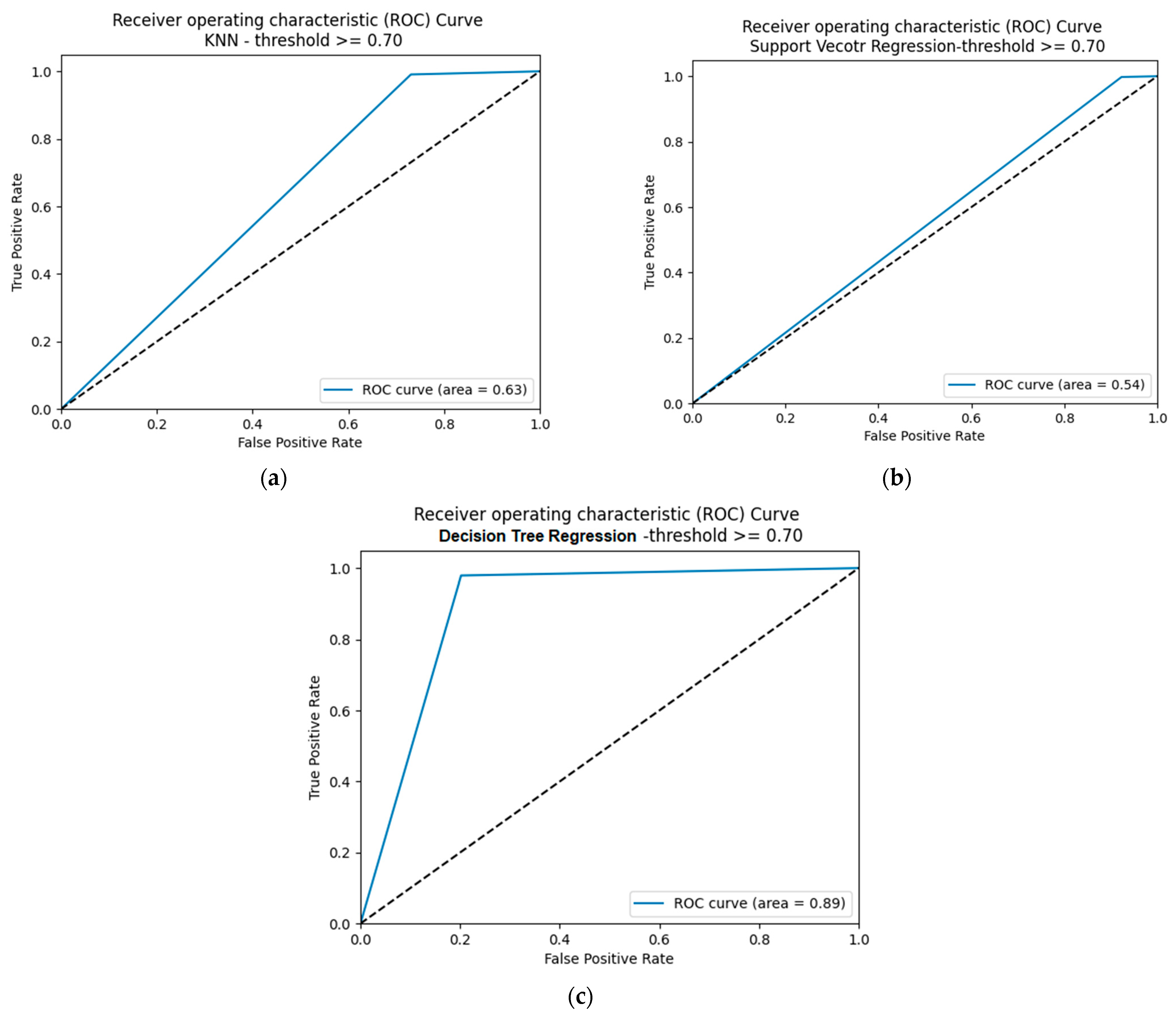
5.2.2. Performance of the SM-kNN, SM-SVR, and SM-DTR Models at Threshold 0.70

The performances of the SM-kNN, SM-SVR, and SM-DTR models were further discussed in terms of precision, recall, and F1-score, at thresholds 0.70, 0.80, and 0.90. The evaluations of the proposed hybrid method at threshold 0.70 are presented in

Table 6. Performance of SM-kNN, SM-DTR, and SM-SVR models at threshold 0.70.

Variable Name	SM-kNN	SM-DTR	SM-SVR
Precision	0.94	0.98	0.93
Recall	0.99	0.98	1.0
F1-score	0.97	0.98	0.96
Accuracy	94%	97%	93%

and Figure 12. Table 6 presents the precision, recall, F1-score, and accuracy values of the classifiers at a threshold of 0.70. It is shown that the SM-DTR model achieved the highest precision of 0.98, while the SM-SVR model had the lowest precision of 0.93. On the other hand, the SM-SVR model achieved the highest recall of 1.00, followed by the SM-kNN and SM-DTR models. However, the SM-DTR model outperformed the other methods with the best F1-score of 0.98, indicating the ability of the DTR classifier to strike a good balance between precision and recall. Moreover, the SM-DTR model had the highest accuracy of 97%, while the SM-kNN and SM-SVR models achieved the accuracies of 94% and 93%, respectively. These metrics are also depicted in Figure 12, which corroborates the results presented in Table 6, highlighting that the DTR is the most accurate classifier for the proposed method, achieving the best precision, F1-score, and accuracy.

The findings discussed above for the SM-kNN, SM-SVR, and SM-DTR models at threshold 0.70 were further validated through the use of Receiver Operating Characteristic (ROC) curves, which provide an accurate measure of the classifiers’ performance. Figure 13 displays the ROC curves for the three classifiers at threshold 0.70. The results depicted in Figure 13 show that the SM-DTR model achieved the highest Area Under the Curve (AUC) ROC of 89%, indicating its superior performance in minimizing the rates of false positives and false negatives. Conversely, the SM-SVR model covers only 54% of the AUC ROC, implying a higher likelihood of erroneous predictions. This observation is consistent with the accuracy results presented in Table 6, where the SM-SVR model recorded the lowest precision compared to the other classifiers. Therefore, it can be concluded that DTR is the most reliable classifier for the proposed method for ontology alignment, while caution should be exercised when employing SVR due to the comparatively lower accuracy and higher possibility of producing false predictions.

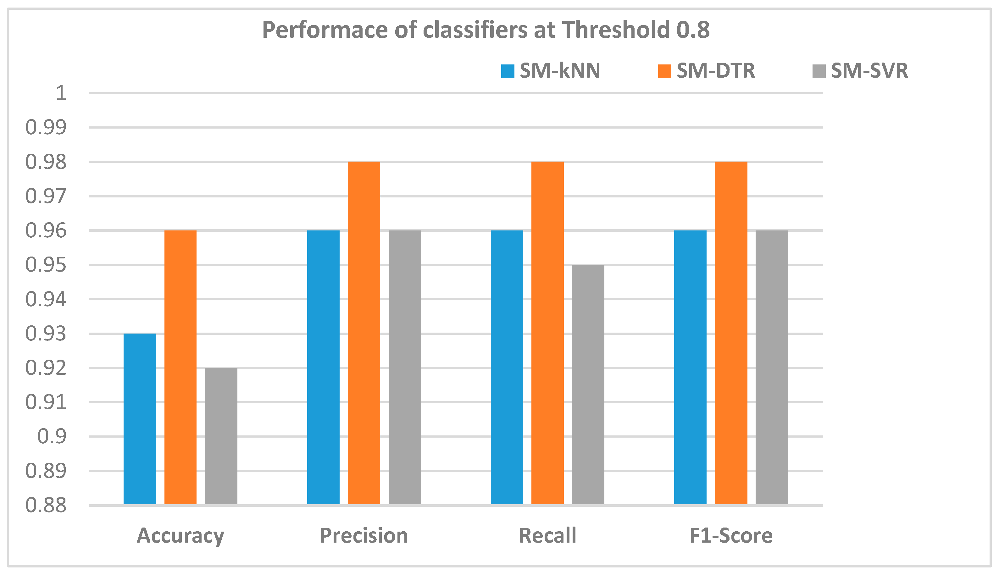
5.2.3. Performance of the SM-kNN, SM-SVR, and SM-DTR Models at Threshold 0.80

The performance of the SM-kNN, SM-SVR, and SM-DTR models at threshold 0.80 is illustrated in

Table 7. Performance of SM-kNN, SM-SVR, and SM-DTR models at threshold 0.80.

Variable Name	SM-kNN	SM-DTR	SM-SVR
Precision	0.96	0.98	0.96
Recall	0.96	0.98	0.95
F1-score	0.96	0.98	0.96
Accuracy	93%	96%	92%

and Figure 14 and Figure 15. It is shown in Figure 14 that the SM-DTR model outperformed the SM-kNN and SM-SVR models in terms of precision, recall, F1-score, and accuracy. Both precision and recall values achieved by the SM-DTR model were 0.98. The accuracy of the SM-DTR model was 96%, compared to 93% and 92% for the SM-kNN and SM-SVR models, respectively. The F1-score for the SM-kNN and SM-SVR models were the same at 0.96 compared to 0.98 for the SM-DTR model. The ROC curves for the three variants of the proposed method were also drawn at threshold 0.80 as shown in Figure 15. It can be observed that the SM-DTR model outperformed the SM-kNN and SM-DTR models, achieving 89% of AUC ROC, thus indicating its superior capability and accuracy. A noteworthy finding is the improved performance of the SM-SVR model that achieved 81% of AUC ROC. The SM-kNN model, on the other hand, ranked third with 80% of AUC ROC with a slight difference from the SM-SVR model’s performance. The results of the ROC curves in Figure 15 are in line with the precision and accuracy values presented in Table 7 and Figure 14. These results further validate the performance of the kNN, SVR, and DTR classifiers and their suitability for the ontology alignment task.

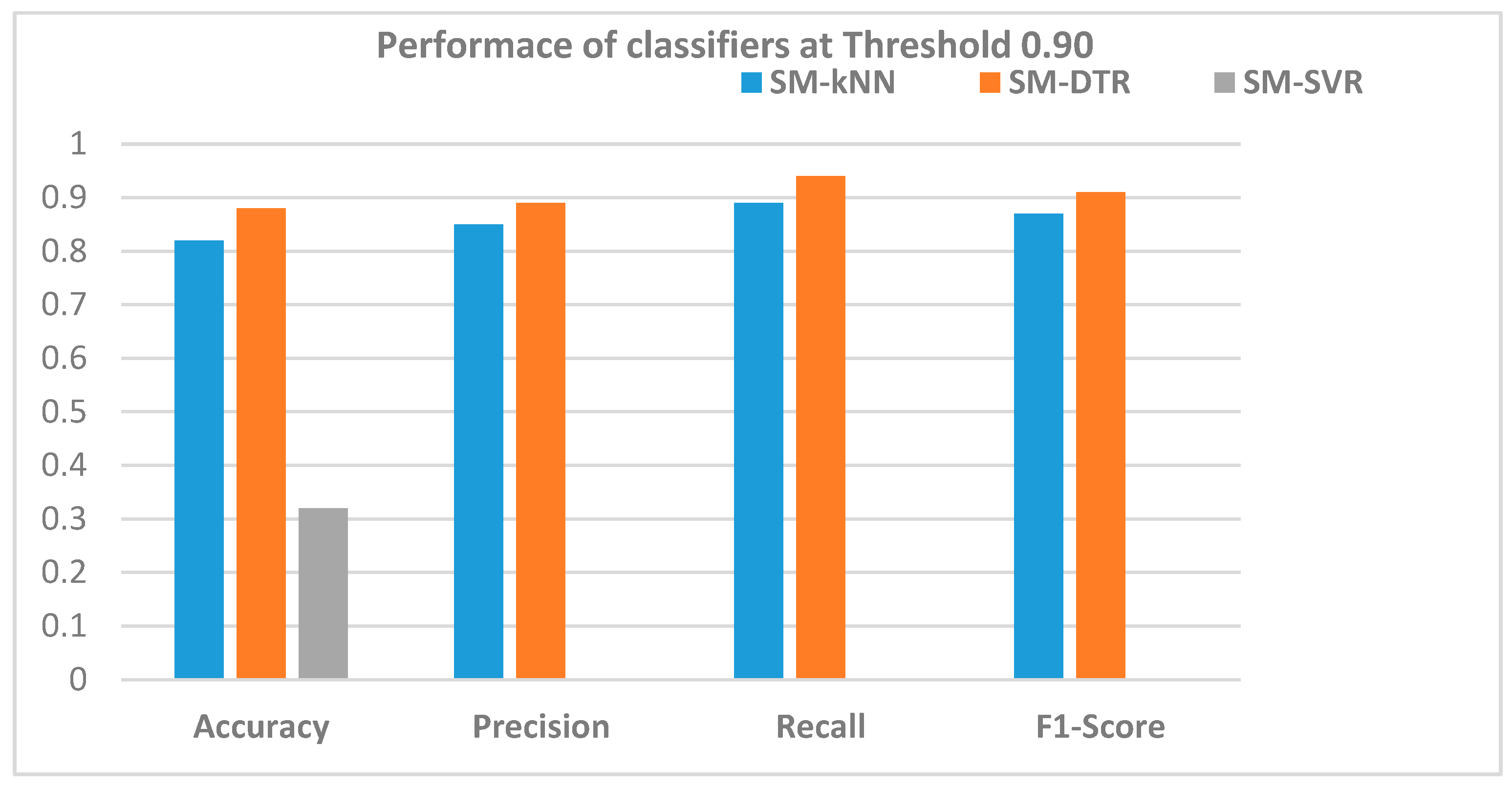
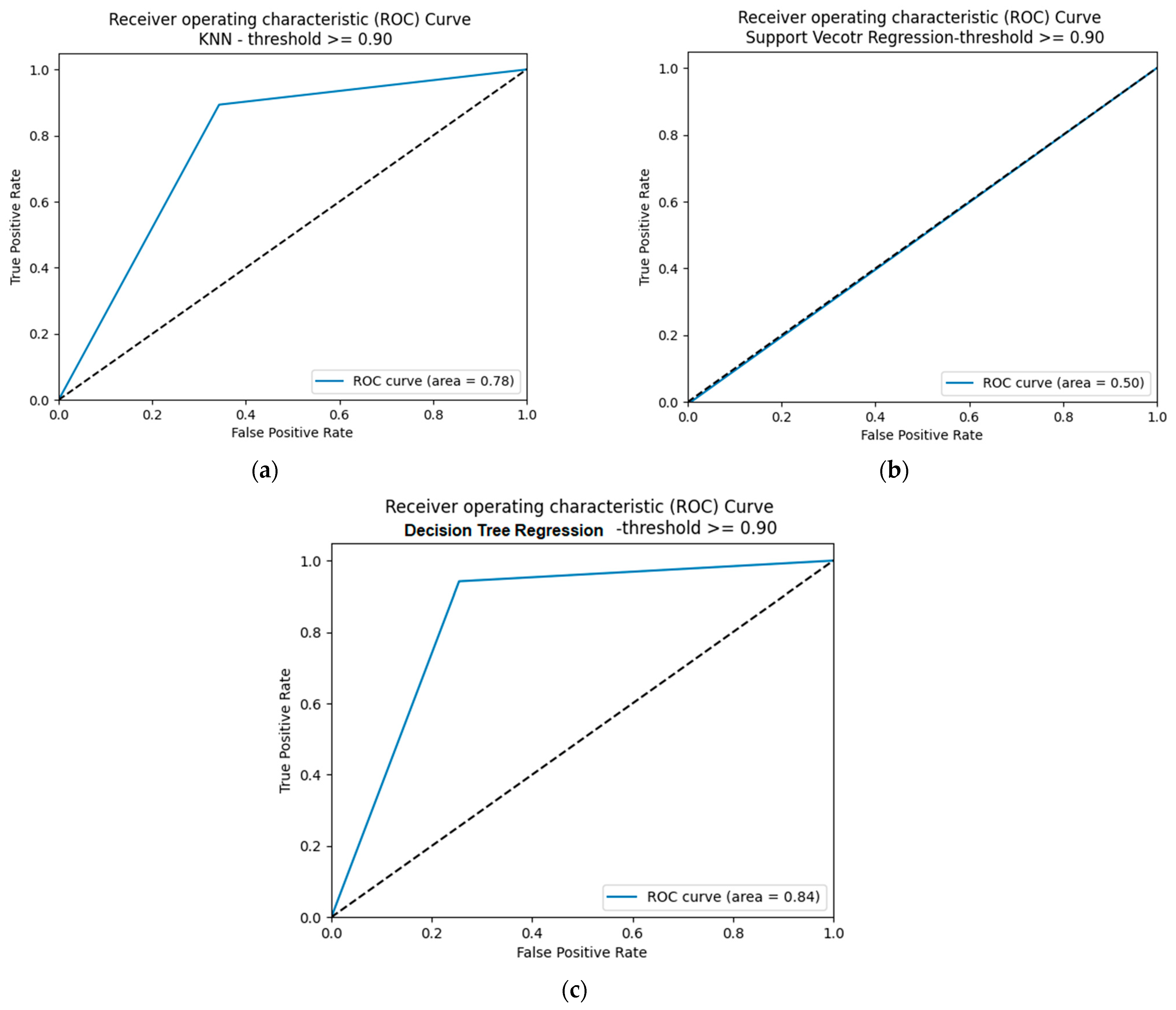
5.2.4. Performance of SM-kNN, SM-SVR, and SM-DTR Models at Threshold 0.90

The threshold was increased to 0.90 to further assess the performance of the three models.

Table 8. Performance of SM-kNN, SM-SVR, and SM-DTR models at threshold 0.90.

Variable Name	SM-kNN	SM-DTR	SM-SVR
Precision	0.85	0.89	0
Recall	0.89	0.94	0
F1-score	0.87	0.91	0
Accuracy	82%	88%	32%

, Figure 16 and Figure 17 displays various performance measures of the SM-kNN, SM-SVR, and SM-DTR models at threshold 0.90.

It is shown in Figure 16 that the SM-SVR model underperformed relative to the other models, exhibiting a low accuracy of 32%, and zero precision, recall, and F1-score. Conversely, the SM-DTR model continued to demonstrate superior performance relative to the others. Notably, the F1-score of SM-DTR was higher than that of SM-kNN model, with a score of 0.91. Additionally, the SM-DTR model exhibited the best accuracy of 88%, while SM-kNN was slightly behind with an accuracy of 82%.

The ROC curves of the SM-kNN, SM-SVR, and SM-DTR models at threshold 0.90 are presented in Figure 17. It is shown in Figure 17 that the SM-DTR model kept its superior performance compared to SM-kNN and SM-SVR with 84% predictions of true positives and true negatives. The performance of the SM-SVR classifier at threshold 0.90 was the worst compared to that at previous thresholds 0.70 and 0.80, while the SM-kNN performance was promising with a slight decrease from its performance at threshold 0.80.

Overall, the results presented above portrayed the SM-DTR as the best model for hybridizing the fuzzy string-matching algorithms and the BERT deep learning model for improved ontology alignment. These results also demonstrated the potential of the kNN classifier as the second-best classifier for combining the strengths of fuzzy string-matching algorithms and the BERT deep learning model to achieve better ontology alignment performance. With regard to the SM-SVR model, the results indicated that it could be used with caution as it may display poor performance at certain threshold levels.

5.3. Analysis of Error Rates of SM-kNN, SM-SVR, and SM-DTR Models

To further evaluate the performance of the three models, we calculated the Mean Squared Error (MSE) and the Root Mean Squared Error (RMSE) for each classifier.

Table 9. MSE and RMSE for the SM-kNN, SM-SVR, and SM-DTR models.

	SM-kNN	SM-DTR	SM-SVR
MSE	0.003	0.003	0.008
RMSE	0.054	0.050	0.091

presents the MSE and RMSE for each classifier.

It is shown in Table 9 that the MSE and RMSE for the three models are very low. The best model was SM-DTR with MSE and RMSE of 0.003 and 0.050, respectively. The SM-SVR model recorded the highest MSE and RMSE of 0.008 and 0.091, respectively. These results are consistent with the above-mentioned findings regarding the performance of the classifiers in terms of precision, recall, F1-score, and accuracy. These results further confirm the SM-DTR as the best model among the three as it exhibited superior performance in terms of error rates and other key metrics.

5.4. Analysis of Processing Time of the SM-kNN, SM-SVR, and SM-DTR Models

Table 10. Running time of SM-kNN, SM-SVR, and SM-DTR models in seconds.

SM-kNN	SM-DTR	SM-SVR
0.0045	0.0011	0.0147

shows the running time of SM-kNN, SM-SVR, and SM-DTR models for performing the 1400 alignments, in seconds.

Table 10 shows that the SM-DTR model achieved the lowest processing time among the three classifiers, aligning the entire dataset in the least amount of time. Conversely, the SM-SVR model obtained the highest processing time of 0.0147 s. The SM-kNN model recorded a processing time that felt between the other two models. Overall, the results indicate that all three models achieved relatively low processing times. However, the SM-DTR model emerged as the most computationally efficient classifier for the proposed method in this study, as it has performed the alignment of the dataset in the least amount of time while also exhibiting superior performance in terms of accuracy and error rates. It was also found that the processing times of all classifiers are relatively low than those of the state-of-the-art systems in OAEI-2022; this is going to be discussed further in the next section. Therefore, in terms of computational efficiency, specifically the running time, our proposed method performs better than some state-of-the-art alignment systems in OAEI 2022. The comparison of our proposed method with the state-of-the-art alignment systems in the OAEI 2022 is presented next.

6. Comparison of the Proposed Method with State-of-the-Art Alignment Systems

In this section, we provide a comparison between our proposed alignment method and state-of-the-art alignment systems that participated in the OAEI 2022. We compare our results to the alignment systems in the Anatomy track of the OAEI 2022 challenge, which involved aligning the mouse and human ontologies, the same used in the experiments in this study to enable an accurate comparison. The web link for accessing information on the Anatomy Track of the OAEI 2022 challenge is given in the Supplementary Materials section of this article. The performances of the participating alignment systems at the OAEI 2022 challenge are presented in

Table 11. Results for OAEI 2022—Anatomy track [59].

Matcher	Runtime	Precision	F-Measure	Recall
ALIN	374	0.984	0.852	0.752
ATMatcher	156	0.978	0.794	0.669
LogMap	9	0.917	0.881	0.848
LogMapBio	1183	0.873	0.895	0.919
LogMapLite	3	0.962	0.828	0.728
LSMatch	20	0.952	0.761	0.634
Matcha	37	0.951	0.941	0.93
ALIOn	26134	0.364	0.407	0.46
SEBMatcher	35602	0.945	0.908	0.874
AMD	160	0.953	0.88	0.817
StringEquiv	-	0.997	0.766	0.622

. Let us recall that the performance of our proposed model, for the metrics reported in Table 11, are provided in Table 6, Table 7 and Table 8 at threshold 0.70, 0.80, and 0.90, respectively, and could not be repeated in Table 11. Therefore, the discussions in this section compare the results in Table 11 to those of this study in Table 6, Table 7 and Table 8.

Table 11 provides the performance of the ontology alignment systems that participated in the OAEI 2022 challenge. The table presents the runtime, precision, F-measure, and recall for each system. It is important to note that the alignment process in OAEI 2022 does not solely rely on lexical alignment but also considers semantic aspects, such as structures, siblings, super- and sub-classes, when generating reference similarity scores between classes. Our proposed method utilized a hybrid approach of the BERT model and fuzzy string-matching algorithms with machine learning regression models to achieve better alignment performance. By taking this approach, we were able to reduce the time for the alignment significantly as evidenced by the low running times of our models in Table 10 compared to the second column of Table 11 for the various state-of-the-art alignment systems. The classifiers used in our approach exhibited faster processing times, demonstrating the efficiency and effectiveness of our method in aligning ontologies. This is a significant advantage, as reducing processing time is crucial in this era of big data where ontologies may include thousands of concepts to process.

In our proposed method, the SM-DTR model demonstrated superior precision performance of 0.98 at both thresholds 0.70 and 0.80 (Table 6 and Table 7). Among the OAEI 2022 matchers, only StringEquiv and ALIN matchers achieved the same precision score. Our SM-kNN and SM-SVR models also performed well in our proposed method, achieving their best precision scores of 0.96. In comparison to the OAEI 2022 matchers in Table 11, our method outperformed the majority, with SM-kNN and SM-SVR coming in fourth place. In terms of recall, our proposed method outperformed the majority of the OAEI 2022 matchers. Specifically, SM-SVR model achieved a perfect recall score of 1.0 at threshold 0.70 (Table 6), surpassing all other matchers in the OAEI 2022 challenge. Our SM-kNN model followed closely with a recall score of 0.99 at the same threshold, which also outperformed the OAEI 2022 matchers. Meanwhile, our SM-DTR model achieved a recall score of 0.98 at thresholds 0.70 and 0.80 (Table 6 and Table 7), which is still superior to most of the OAEI 2022 matchers in Table 11. Notably, even at the most stringent threshold of 0.90, our SM-DTR still outperformed all OAEI 2022 matchers with a record performance of 0.94 in terms of recall. Our SM-kNN model’s recall of 0.89 (Table 8) placed it at the third position behind the Matcha and LogMapBio systems (Table 11), which achieved a recall of 0.93 and 0.919, respectively. Although our SM-SVR model did not perform as well at threshold 0.90, it still demonstrated impressive performance at thresholds 0.80 and 0.70 (Table 6 and Table 7) compared to the alignment systems in Table 11. Regarding the F-measure, our proposed method achieved superior results compared to the OAEI 2022 systems. Our SM-DTR model recorded the best F-measure score of 0.98 at both thresholds 0.70 and 0.80 (Table 6 and Table 7), outperforming the best OAEI 2022 system, namely, Matcha, which achieved an F-measure score of 0.94 (Table 11). These results demonstrate the effectiveness of our proposed method in accurately aligning ontologies, outperforming the state-of-the-art alignment systems in terms of recall and F-measure.

In addition to the above-mentioned metrics used in the OAEI 2022 challenge, our proposed method was also evaluated based on the accuracy (Table 6, Table 7 and Table 8) as an important measure of alignment systems’ performance. Additionally, error rates (MSE and RMSE) were also measured for all three proposed models. These additional metrics provides a more comprehensive evaluation of alignment systems’ performance compared to the OAEI 2022 challenge. Based on the discussions above, this study has proposed a novel method that successfully hybridized fuzzy string-matching algorithms and BERT deep learning model with machine learning regression classifiers for improved ontology alignment performances and the proposed method has outperformed the state-of-the-art alignment systems. In particular, our SM-DTR model based on DTR achieved the best overall performance at different thresholds. Our SM-kNN model came in second place, also demonstrating strong performance at different thresholds, whereas our SM-SVR model struggled at a stricter threshold like 0.90 but performed very well at lower thresholds. Overall, our method offers significant improvements in ontology alignment performance compared to existing systems.

7. Conclusions and Future Work

In this study, we examined the benefits of fuzzy string-matching algorithms in the ontology alignment process and demonstrated how their effectiveness can be enhanced by incorporating semantic information using BERT. We evaluated the performance of four fuzzy string-matching algorithms on their own and found that they perform less accurately at higher thresholds. However, our proposed method that combined similarity scores obtained from fuzzy string-matching algorithms and BERT achieved very promising results, outperforming fuzzy string-matching algorithms and some of the state-of-the-art alignment systems in the OAEI 2022 ontology alignment challenge. To evaluate the effectiveness of the proposed method, we conducted experiments at three different thresholds and compared the performance of three hybrid models, namely, SM-kNN, SM-SVR, and SM-DTR. Various metrics including precision, recall, F1-score, Mean Square Error (MSE), and Root Mean Square Error (RMSE), and running time were used to evaluate the performance of the hybrid models. The experimental results showed that SM-DTR was the most effective model for ontology alignment that considers both lexical and semantic characteristics of ontologies. With best-of precision, recall, and F1-scores of 0.98, SM-DTR outperformed the other models, followed by SM-kNN, which achieved a best F1-score of 0.97. Moreover, SM-DTR showed the highest accuracy of 96% compared to the other models.

The results of the proposed method can be used in many applications. One application is the integration and reuse of ontologies into custom software applications. Another possible application includes facilitating ontologies merging in which alignment process is crucial to build upon.

In terms of future work, several avenues can be explored to enhance the versatility and adaptability of our approach. One direction involves investigating the integration of our proposed model with complementary techniques, which would offer increased flexibility to support languages other than English. Additionally, leveraging the fine-tuning capabilities of BERT, a re-trained model tailored for specific purposes, such as aligning individuals or logical axioms, holds promise for custom applications. By pursuing these potential research directions, our model can be further optimized and refined to address a wider array of language-related challenges and requirements.

References

1. Shadbolt, N.; Berners-Lee, T.; Hall, W. The semantic web revisited. IEEE Intell. Syst. 2006, 21, 96–101. [Google Scholar] [CrossRef] [Green Version]
2. Gruber, T.R. A translation approach to portable ontology specifications. Knowl. Acquis. 1993, 5, 199–220. [Google Scholar] [CrossRef]
3. Shojaee-Mend, H.; Ayatollahi, H.; Abdolahadi, A. Developing a mobile-based disease ontology for traditional Persian medicine. Inform. Med. Unlocked 2020, 20, 100353. [Google Scholar] [CrossRef]
4. Hu, S.; Wang, H.; She, C.; Wang, J. Agont: Ontology for Agriculture Internet of Things; Springer: Berlin/Heidelberg, Germany, 2011. [Google Scholar]
5. Reedoy, A.V.; Dayal, S.B.; Govender, P.; Fonou-Dombeu, J.V. An ontology for smart home design. In Proceedings of the 2021 International Conference on Artificial Intelligence, Big Data, Computing and Data Communication Systems (icABCD), Durban, South Africa, 5–6 August 2021. [Google Scholar]
6. Esbjörn-Hargens, S. An ontology of climate change. J. Integral Theory Pract. 2010, 5, 143–174. [Google Scholar]
7. Bouyerbou, H.; Bechkoum, K.; Lepage, R. Geographic ontology for major disasters: Methodology and implementation. Int. J. Disaster Risk Reduct. 2019, 34, 232–242. [Google Scholar] [CrossRef]
8. Elsaleh, T.; Enshaeifar, S.; Rezvani, R.; Acton, S.T.; Janeiko, V.; Bermudez-Edo, M. IoT-Stream: A lightweight ontology for internet of things data streams and its use with data analytics and event detection services. Sensors 2020, 20, 953. [Google Scholar] [CrossRef] [Green Version]
9. Alsanad, A.A.; Chikh, A.; Mirza, A. A domain ontology for software requirements change management in global software development environment. IEEE Access 2019, 7, 49352–49361. [Google Scholar] [CrossRef]
10. Al-Zebari, A.; Zebari, S.; Jacksi, K. Football Ontology Construction using Oriented Programming. J. Appl. Sci. Technol. Trends 2020, 1, 24–30. [Google Scholar] [CrossRef]
11. Uschold, M.; Healy, M.J.; Keith, E.W.; Clark, P.; Woods, S. Ontology reuse and application. In Formal Ontology in Information Systems; IOS Press: Amsterdam, The Netherlands, 1998. [Google Scholar]
12. Jiménez, A.; Suárez-Figueroa, M.C.; Mateos, A.; Gomez-Perez, A.; Fernandez-Lopez, M. A maut approach for reusing domain ontologies on the basis of the neon methodology. Int. J. Inf. Technol. Decis. Mak. 2013, 12, 945–968. [Google Scholar] [CrossRef] [Green Version]
13. Nkisi-Orji, I.; Wiratunga, N.; Massie, S.; Hui, K.-Y.; Heaven, R. Ontology Alignment Based on Word Embedding and Random Forest Classification; Springer: Cham, Switzerland, 2019. [Google Scholar]
14. Hughes, T.C.; Ashpole, B.C. The Semantics of Ontology Alignment; Lockheed Martin Advanced Technology Labs: Cherry Hill, NJ, USA, 2004. [Google Scholar]
15. Ouali, I.; Ghozzi, F.; Taktak, R.; Sassi, M.S.H.S. Ontology alignment using stable matching. Procedia Comput. Sci. 2019, 159, 746–755. [Google Scholar] [CrossRef]
16. Liu, X.; Tong, Q.; Liu, X.; Qin, Z. Ontology matching: State of the art, future challenges, and thinking based on utilized information. IEEE Access 2021, 9, 91235–91243. [Google Scholar] [CrossRef]
17. de Lourdes Martínez-Villaseñor, M.; González-Mendoza, M. Fuzzy-Based Approach of Concept Alignment; Springer: Cham, Switzerland, 2017. [Google Scholar]
18. Cochez, M. Locality-sensitive hashing for massive string-based ontology matching. In Proceedings of the 2014 IEEE/WIC/ACM International Joint Conferences on Web Intelligence (WI) and Intelligent Agent Technologies (IAT), Warsaw, Poland, 11–14 August 2014. [Google Scholar]
19. Cheatham, M.; Hitzler, P. String similarity metrics for ontology alignment. In Proceedings of the Semantic Web–Iswc 2013: 12th International Semantic Web Conference, Sydney, Australia, 21–25 October 2013; Springer: Berlin/Heidelberg, Germany, 2013. [Google Scholar]
20. Rudwan, M.S.M.; Fonou-Dombeu, J.V. Ontology Reuse: Neural Network-Based Measurement of Concepts Representations and Similarities in Ontology Corpus. In Proceedings of the 2022 International Conference on Artificial Intelligence, Big Data, Computing and Data Communication Systems (icABCD), Durban, South Africa, 4–5 August 2022. [Google Scholar]
21. Rudwan, M.S.M.; Fonou-Dombeu, J.V. Machine Learning Selection of Candidate Ontologies for Automatic Extraction of Context Words and Axioms from Ontology Corpus; Springer: Cham, Switzerland, 2022. [Google Scholar]
22. Megdiche, I.; Teste, O.; Trojahn, C. An Extensible Linear Approach For Holistic Ontology Matching; Springer: Cham, Switzerland, 2016. [Google Scholar]
23. Chu, S.C.; Xue, X.; Pan, J.S.; Wu, X. Optimizing ontology alignment in vector space. J. Internet Technol. 2020, 21, 15–22. [Google Scholar]
24. Patel, A.; Jain, S. A novel approach to discover ontology alignment. Recent Adv. Comput. Sci. Commun. (Former. Recent Pat. Comput. Sci.) 2021, 14, 273–281. [Google Scholar] [CrossRef]
25. Liu, W.; Xue, X.; Wu, Z.; Istanda, V. Aggregating Similarity Measures for Optimizing Ontology Alignment. J. Netw. Intell. 2022, 7, 36–44. [Google Scholar]
26. Mani, S.; Annadurai, S. An Improved Structural-Based Ontology Matching Approach Using Similarity Spreading. Int. J. Semant. Web Inf. Syst. (IJSWIS) 2022, 18, 1–17. [Google Scholar] [CrossRef]
27. Zhou, X.; Lv, Q.; Geng, A. Matching heterogeneous ontologies based on multi-strategy adaptive co-firefly algorithm. Knowl. Inf. Syst. 2023, 65, 2619–2644. [Google Scholar] [CrossRef]
28. Şentürk, F.; Aytac, V. A Graph-Based Ontology Matching Framework. New Gener. Comput. 2023, 1–19. [Google Scholar] [CrossRef]
29. Bulygin, L. Combining lexical and semantic similarity measures with machine learning approach for ontology and schema matching problem. In Proceedings of the XX International Conference “Data Analytics and Management in Data Intensive Domains”(DAMDID/RCDL’2018), Moscow, Russia, 9–12 October 2018. [Google Scholar]
30. Bento, A.; Zouaq, A.; Gagnon, M. Ontology matching using convolutional neural networks. In Proceedings of the Twelfth Language Resources and Evaluation Conference, Marseille, France, 11–16 May 2020. [Google Scholar]
31. Faria, D.; Pesquita, C.; Santos, E.; Palmonari, M.; Cruz, I.F.; Couto, F.M. The Agreementmakerlight Ontology Matching System; Springer: Cham, Switzerland, 2013. [Google Scholar]
32. Jiménez-Ruiz, E.; Grau, B.C. Logmap: Logic-Based and Scalable Ontology Matching; Springer: Cham, Switzerland, 2011. [Google Scholar]
33. Xiang, Y.; Zhang, Z.; Chen, J.; Chen, X.; Lin, Z.; Zheng, Y. OntoEA: Ontology-guided entity alignment via joint knowledge graph embedding. arXiv 2021, arXiv:2105.07688. [Google Scholar]
34. Karimi, H.; Kamandi, A. A learning-based ontology alignment approach using inductive logic programming. Expert Syst. Appl. 2019, 125, 412–424. [Google Scholar] [CrossRef]
35. Wang, L.L.; Bhagavatula, C.; Neumann, M.; Lo, K.; Wilhelm, C.; Ammar, W. Ontology alignment in the biomedical domain using entity definitions and context. arXiv 2018, arXiv:1806.07976. [Google Scholar]
36. Khoudja, M.A.; Fareh, M.; Bouarfa, H. Ontology matching using neural networks: Survey and analysis. In Proceedings of the 2018 International Conference on Applied Smart Systems (ICASS), Medea, Algeria, 24–25 November 2018. [Google Scholar]
37. Sun, Y.; Ma, L.; Wang, S. A comparative evaluation of string similarity metrics for ontology alignment. J. Inf. Comput. Sci. 2015, 12, 957–964. [Google Scholar] [CrossRef]
38. Cross, V. Semantic Similarity: A Key to Ontology Alignment. 2018. Available online: http://disi.unitn.it/~pavel/om2018/papers/om2018_STpaper1.pdf (accessed on 1 May 2023).
39. Santisteban, J.; Tejada-Cárcamo, J. Unilateral Jaccard Similarity Coefficient. 2015. Available online: https://ceur-ws.org/Vol-1393/paper-10.pdf (accessed on 1 May 2023).
40. He, Y.; Chen, J.; Antonyrajah, D.; Horrocks, I. BERTMap: A BERT-based ontology alignment system. Proc. AAAI Conf. Artif. Intell. 2022, 36, 5684–5691. [Google Scholar] [CrossRef]
41. Neutel, S.; De Boer, M.H.T. Towards Automatic Ontology Alignment using BERT. In Proceedings of the AAAI Spring Symposium: Combining Machine Learning with Knowledge Engineering, Palo Alto, CA, USA, 22–24 March 2021. [Google Scholar]
42. He, Y.; Chen, J. Biomedical ontology alignment with BERT. In Proceedings of the 16th International Workshop on Ontology Matching co-located with the 20th International Semantic Web Conference (ISWC 2021), Virtual Event, 25 October 2021. [Google Scholar]
43. Bajaj, G.; Nguyen, V.; Wijesiriwardene, T.; Yip, H.Y.; Javangula, V.; Parthasarathy, S.; Sheth, A.; Bodenreider, O. Evaluating Biomedical BERT Models for Vocabulary Alignment at Scale in the UMLS Metathesaurus. arXiv 2021, arXiv:2109.13348. [Google Scholar]
44. Keil, J.M. Efficient Bounded Jaro-Winkler Similarity Based Search; Gesellschaft für Informatik: Bonns, Germany, 2019. [Google Scholar]
45. Zhang, S.; Hu, Y.; Bian, G. Research on string similarity algorithm based on Levenshtein Distance. In Proceedings of the 2017 IEEE 2nd Advanced Information Technology, Electronic and Automation Control Conference (IAEAC), Chongqing, China, 25–26 March 2017. [Google Scholar]
46. Bergroth, L.; Hakonen, H.; Raita, T. A survey of longest common subsequence algorithms. In Proceedings of the Seventh International Symposium on String Processing and Information Retrieval, SPIRE 2000, A Curuna, Spain, 27–29 September 2000. [Google Scholar]
47. Devlin, J.; Chang, M.W.; Lee, K.; Toutanova, K. Bert: Pre-training of deep bidirectional transformers for language understanding. arXiv 2018, arXiv:1810.04805. [Google Scholar]
48. Vaswani, A.; Shazeer, N.; Parmar, N.; Uszkoreit, J.; Jones, L.; Gomez, A.N.; Kaiser, Ł.; Polosukhin, I. Attention is all you need. In Proceedings of the 31st Conference on Neural Information Processing Systems (NIPS 2017), Long Beach, CA, USA, 4–9 December 2017. [Google Scholar]
49. Radford, A.; Narasimhan, K.; Salimans, T.; Sutskever, I. Improving Language Understanding with Unsupervised Learning. 2018. Available online: https://openai.com/research/language-unsupervised (accessed on 1 May 2023).
50. Zhang, Z. Introduction to machine learning: k-nearest neighbors. Ann. Transl. Med. 2016, 4, 218. [Google Scholar] [CrossRef] [PubMed] [Green Version]
51. Modaresi, F.; Araghinejad, S.; Ebrahimi, K. A comparative assessment of artificial neural network, generalized regression neural network, least-square support vector regression, and K-nearest neighbor regression for monthly streamflow forecasting in linear and nonlinear conditions. Water Resour. Manag. 2018, 32, 243–258. [Google Scholar] [CrossRef]
52. Hu, C.; Jain, G.; Zhang, P.; Schmidt, C.; Gomadam, P.; Gorka, T.S. Data-driven method based on particle swarm optimization and k-nearest neighbor regression for estimating capacity of lithium-ion battery. Appl. Energy 2014, 129, 49–55. [Google Scholar] [CrossRef]
53. Awad, M.; Khanna, R. Support Vector Regression. Efficient Learning Machines: Theories, Concepts, and Applications for Engineers and System Designers; Apress: Berkeley, CA, USA, 2015; pp. 67–80. [Google Scholar]
54. Pekel, E. Estimation of soil moisture using decision tree regression. Theor. Appl. Climatol. 2020, 139, 1111–1119. [Google Scholar] [CrossRef]
55. Swetapadma, A.; Yadav, A. A novel decision tree regression-based fault distance estimation scheme for transmission lines. IEEE Trans. Power Deliv. 2016, 32, 234–245. [Google Scholar] [CrossRef]
56. Xue, X.; Yang, C.; Jiang, C.; Tsai, P.-W.; Mao, G.; Zhu, H. Optimizing ontology alignment through linkage learning on entity correspondences. Complexity 2021, 2021, 5574732. [Google Scholar] [CrossRef]
57. Hariri, B.B.; Sayyadi, H.; Abolhassani, H.; Esmaili, K.S. Combining Ontology Alignment Metrics Using the Data Mining Techniques. 2006. Available online: https://ceur-ws.org/Vol-210/paper17.pdf (accessed on 1 May 2023).
58. Zhu, X.; Zhang, S.; Jin, Z.; Zhang, Z.; Xu, Z. Missing value estimation for mixed-attribute data sets. IEEE Trans. Knowl. Data Eng. 2010, 23, 110–121. [Google Scholar] [CrossRef]
59. OAEI. Results—Anatomoy Track. 2022. Available online: http://oaei.ontologymatching.org/2022/results/anatomy/index.html (accessed on 1 April 2023).
Figure 1. BERT model showing its two phases: pre-training and fine-tuning [47].
Futureinternet 15 00229 g001
Figure 2. Proposed model that hybridizes fuzzy string matching and machine learning for automatic ontology alignment.
Futureinternet 15 00229 g002
Figure 3. Confusion matrix for fuzzy string-matching algorithms and BERT at threshold 0.70. (a) Levenshtein, (b) LCS, (c) Jaccard, (d) Jaro–Winkler, (e) BERT.
Futureinternet 15 00229 g003
Figure 4. Confusion matrix for fuzzy string-matching algorithms and BERT at threshold 0.80. (a) Levenshtein, (b)LCS, (c) Jaccard, (d) Jaro–Winkler, (e) BERT.
Futureinternet 15 00229 g004
Figure 5. Confusion matrix for fuzzy string-matching algorithms and BERT at threshold 0.90. (a) Levenshtein, (b) LCS, (c) Jaccard, (d) Jaro–Winkler, (e) BERT.
Futureinternet 15 00229 g005
Figure 6. Confusion matrix for SM-kNN, SM-SVR, and SM-DTR models at threshold 0.70. (a) SM-kNN, (b) SM-SVR, (c) SM-DTR.
Futureinternet 15 00229 g006
Figure 7. Confusion matrix for SM-kNN, SM-SVR, and SM-DTR models at threshold 0.80. (a) SM-kNN, (b) SM-SVR, (c) SM-DTR.
Futureinternet 15 00229 g007
Figure 8. Confusion matrix for SM-KNN, SM-SVR, and SM-DTR models at threshold 0.90. (a) SM-KNN, (b) SM-SVR, (c) SM-DTR.
Futureinternet 15 00229 g008
Figure 9. Scatterplot diagram of similarity cores predicted by SM-kNN vs. AML reference scores.
Futureinternet 15 00229 g009
Figure 10. Scatterplot diagram of similarity cores predicted by SM-SVR vs. AML reference scores.
Futureinternet 15 00229 g010
Figure 11. Scatterplot diagram of similarity cores predicted by SM-DTR vs. AML reference scores.
Futureinternet 15 00229 g011
Figure 12. Accuracy, precision, recall, and F1-score for SM-kNN, SM-SVR, and SM-DTR models at threshold 0.70.
Futureinternet 15 00229 g012
Figure 13. ROC curves for SM-kNN, SM-SVR, and SM-DTR models at threshold 0.70. (a) SM-kNN, (b) SM-SVR, (c) SM-DTR.
Futureinternet 15 00229 g013
Figure 14. Accuracy, precision, recall, and F1-score for SM-kNN, SM-SVR, and SM-DTR models at threshold 0.80.
Futureinternet 15 00229 g014
Figure 15. ROC curves of SM-kNN, SM-SVR, and SM-DTR models at threshold 0.80. (a) SM-kNN, (b) SM-SVR, (c) SM-DTR.
Futureinternet 15 00229 g015aFutureinternet 15 00229 g015b
Figure 16. Accuracy, precision, recall, and F1-score of SM-kNN, SM-SVR, and SM-DTR models at threshold 0.90.
Futureinternet 15 00229 g016
Figure 17. ROC curves of SM-kNN, SM-SVR, and SM-DTR models at threshold 0.90. (a) SM-kNN, (b) SM-SVR, (c) SM-DTR.
Futureinternet 15 00229 g017