Dual-Channel Feature Enhanced Collaborative Filtering Recommendation Algorithm

Abstract

The dual-channel graph collaborative filtering recommendation algorithm (DCCF) suppresses the over-smoothing problem and overcomes the problem of expansion in local structures only in graph collaborative filtering. However, DCCF has the following problems: the fixed threshold of transfer probability leads to a decrease in filtering effect of neighborhood information; the K-means clustering algorithm is prone to trapping clustering results into local optima, resulting in incomplete global interaction graphs; and the impact of time factors on the predicted results was not considered. To solve these problems, a dual-channel feature enhanced collaborative filtering recommendation algorithm (DCFECF) is proposed. Firstly, the self-attention mechanism and weighted average method are used to calculate the threshold of neighborhood transition probability for each order in local convolutional channels; secondly, the K-means++ clustering algorithm is used to determine the clustering center in the global convolutional channel, and the fuzzy C-means clustering algorithm is used for clustering to solve the local optimal problem; then, time factor is introduced to further improve predicted results, making them more accurate. Comparative experiments using normalized discounted cumulative gain (NDCG) and recall as evaluation metrics on three publicly available datasets showed that DCFECF improved by up to 2.3% and 4.1% on two metrics compared to DCCF.

1. Introduction

The rapid development of the internet has led to the rapid growth of different types of data, resulting in the problem of “information overload”. It is not easy for users to efficiently select the content they are interested in when facing massive amounts of network data. The recommendation model [1] is a reliable and effective technique that can recommend content of interest to users based on their historical behavior records, thereby alleviating the problem of “information overload”. Collaborative filtering is widely used in recommendation models, which is a recommendation algorithm based on user behavior data. In recent years, driven by the demand for relationship modeling in recommendation task scenarios, building collaborative filtering recommendation models [2,3] using graph convolution networks has become mainstream.

However, the collaborative filtering model based on graph convolution networks has the following problems: Firstly, graph convolution networks have the over-smoothing problem [4,5]. The node features transferred to the deep layer gradually become similar, and the preference features in the recommendation process become homogeneous, which reduces the model performance. Secondly, the adjacency matrix is used to express the interaction relationship between users and items, focusing on the feature aggregation [6] of the local neighborhood, and it is impossible to mine the interaction pattern between nodes through the overall structure of the graph.

The existing solutions represented by the dual-channel graph collaborative filtering recommendation algorithm [7] (DCCF), on the one hand, introduce the transition matrix, set the transition probability threshold, determine the neighborhood range of nodes, and adopt a single-layer network structure to suppress the over-smoothing problem in the graph convolution network iteration process; on the other hand, clustering is used to construct a global interaction graph, model the potential interaction between nodes, supplement global information, and overcome the problem that the interaction information is limited to the local neighborhood.

The above solution has the following problems: firstly, the transition probability threshold is set to a fixed value and does not dynamically change the transition probability threshold based on different samples, which will reduce the accuracy of the prediction results; secondly, the K-means clustering algorithm used by DCCF for clustering is sensitive to the initial clustering center, which makes it easy for the clustering result to fall into local optimum and is not conducive to the construction of a comprehensive global interaction graph; finally, users’ interests will change over time and DCCF does not consider the impact of time factors on user preferences.

To solve the above problems, this paper proposes a dual-channel feature enhanced collaborative filtering recommendation algorithm (DCFECF). The contributions of this paper are summarized as follows:

• In the local convolutional channel, we introduce a self-attention mechanism to calculate the weight value of each edge and use the weighted average method to calculate the threshold of neighborhood transition probability for each order. The transfer probability threshold is converted from a fixed value to a dynamic value.
• In the global convolutional channel, we use the K-means++ clustering algorithm to determine the clustering center and then use the fuzzy C-means clustering algorithm to replace the K-means clustering algorithm for clustering, solving the local optimal problem and enabling the construction of a more comprehensive global interaction graph.
• At the same time, we introduce a time factor into the model and modify the existing time factor expression to further improve the predicted results.

2. Related Work

2.1. Collaborative Filtering Model Based on Graph Convolution Network

In the process of building the collaborative filtering model, the graph convolution network is introduced: on the one hand, by taking users and items as nodes, users’ scoring, browsing, and other behaviors in history can be seen as the “connecting edge” between the two, and graph structure can be used to express data, which is closer to the real scene; on the other hand, graph convolutional networks have strong advantages in mining connections between nodes and learning to represent graphical data. Introducing the graph convolution network into collaborative filtering can further improve the performance of algorithm recommendation.

The collaborative filtering model based on the graph convolution network has the over-smoothing problem and the interaction information is limited to the local neighborhood. The GC-MC model [8] introduces graph convolution operation for the first time, using neighbor node information as a vector representation of user nodes and item nodes. The NGCF model [9] utilizes a multi-layer graph convolutional network to extract feature information. Both GC-MC and NGCF introduce graph convolutional networks into the process of vector embedding, utilizing the added feature information of neighboring nodes to enhance the model’s expression ability, but there is still an over-smoothing problem. The LR-GCCF model [10] is simplified on the basis of the NGCF model, removing some components that may affect recommendation performance and incorporating residual connections to solve the over-smoothing problem. The DHCF model [11] constructs hypergraphs, expresses node neighborhood information, and proposes new graph convolution operations. The DCCF model divides the vector expression update process between user nodes and item nodes into local convolutional channels and global convolutional channels, performing different information aggregation tasks. In the local convolutional channel, a single-layer network structure is used to suppress the over-smoothing problem in the iterative process of graph convolutional networks; in the global convolution channel, K-means clustering is used to construct the global interaction graph to supplement the global information and overcome the problem that the interaction information is limited to the local neighborhood.

2.2. Clustering Algorithm

Clustering algorithms are an unsupervised learning method, which are divided into hard clustering and soft clustering. The membership degree of the hard clustering algorithm only has two values: 0 and 1. The K-means clustering algorithm [12] is one of the classic algorithms. The K-means++ clustering algorithm is improved on the basis of the K-means clustering algorithm.

Soft clustering algorithms divide data by similarity and categorize data with high similarity. The fuzzy C-means (FCM) [13] clustering algorithm is a distance-based soft clustering algorithm that assigns each data point to multiple cluster centers and assigns a membership degree to each data point.

Assuming user dataset $U=\left\{u_1,u_2,\dots ,u_n\right\}$ with $m$ features, set as $u_i=\left\{r_{i1},r_{i2},\cdots ,r_{im}\right\}$. If users are divided into $k$ clusters with a cluster center of $Z=\left\{z_1,z_2,\cdots ,z_k\right\}$, a fuzzy matrix $W={\left(w_{\mathrm{ij}}\right)}_{n\times k}$ can be constructed, where $w_{ij}\in \left[0,1\right]$ represents the membership degree of the $i$-th user belonging to the $j$-th cluster. FCM uses the sum of squared errors function as the objective function to minimize the objective function and divide $n$ users into $k$ clusters. The definition formula and constraint conditions of the objective function are shown in Equations (1) and (2).

$$J_k\left(W,Z\right)={\displaystyle \sum _{a=1}^n{\displaystyle \sum _{b=1}^k{\left(w_{ab}\right)}^{\rho }{\Vert u_a-z_b\Vert }^2}}$$

(1)

$${\displaystyle \sum _{b=1}^k{w}_{ab}=1,a=1,2,3,\cdots ,n}$$

(2)

where $\rho$ is the fuzzy index, usually taken as 2. Using the Lagrangian multiplier method, calculate the extremum of the objective function, obtain the partial derivatives of variables $w_{ij}$ and $z_j$, respectively, and obtain the membership degree and cluster center according to Equations (3) and (4).

$$w_{ab}={\left[\frac{{\Vert u_a-z_b\Vert }^{\frac{2}{\rho -1}}}{{\displaystyle \sum _{j=1}^k{\Vert u_a-z_j\Vert }^{\frac{2}{\rho -1}}}}\right]}^{-1}$$

(3)

$$z_b=\frac{{\displaystyle \sum _{i=1}^n{\left(w_{ab}\right)}^{\rho }{u}_i}}{{\displaystyle \sum _{i=1}^n{\left(w_{ab}\right)}^{\rho }}}$$

(4)

Before using FCM, we need to determine the fuzzy index $\rho$ and the limiting iteration index $eps$. After obtaining the final membership matrix, the partition of the cluster is obtained through membership, and users are assigned to the cluster with the highest membership, resulting in the highest similarity among users in the same user cluster.

3. DCFECF Model

3.1. Model Prediction Process and Framework

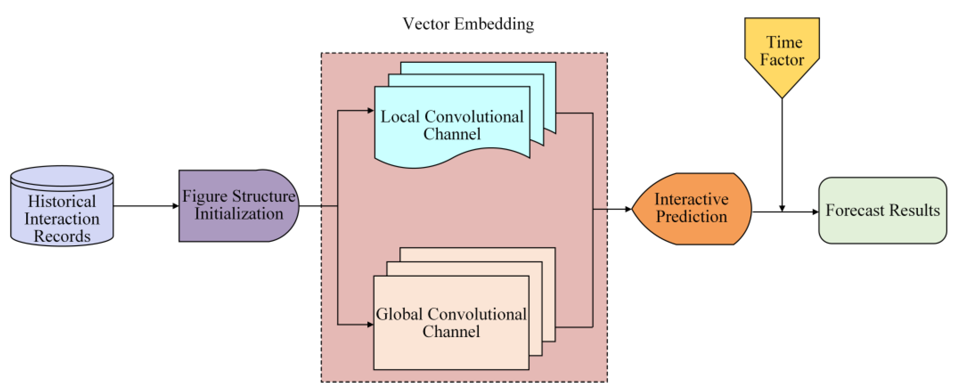
Compared with the DCCF model, the DCFECF model adds the introduction of the time factor. Its prediction process is shown in Figure 1. Firstly, the initial graph structure is exported from the historical interaction record, including the bipartite interactive graph between users and items, and the initialization vector expression of nodes in the graph. Secondly, local and global convolutional channels are used to express the interaction relationship between higher-order nodes. Then, in the form of vector inner product, interactions that were not observed in historical interaction records are predicted. Finally, the time factor is added to the interactive prediction to further improve the prediction results.

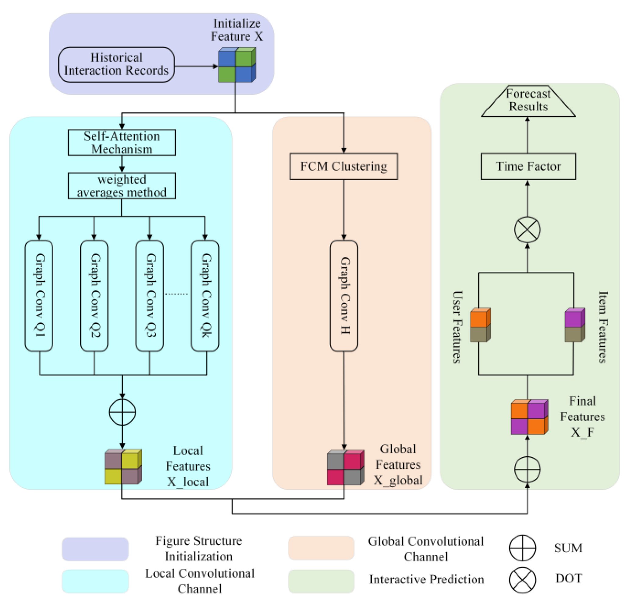
Based on the above analysis, the structure of the DCFECF model is shown in Figure 2, which is mainly divided into three parts: the local convolutional channel, the global convolutional channel, and the interactive prediction module.

Where the local convolutional channel aggregates the feature information in the local neighborhood structure, it uses a state transition matrix to determine the high-order neighborhood range of nodes. By using the self-attention mechanism and the weighted average method, the threshold of the neighborhood transition probability of each order is obtained. Then, a single-layer graph convolutional network is used to aggregate local information between user nodes and item nodes, thereby suppressing the over-smoothing problem. In the global convolution channel, the fuzzy C-means clustering algorithm optimized by K-means++ clustering is used for clustering, and a global interaction graph is constructed. According to the feature similarity between nodes, neighbor nodes with similar features are selected for user and item nodes from the global perspective to supplement global information and overcome the problem that interaction information is limited to the local neighborhood. In the interaction prediction stage, local and global information are integrated, and the inner product of the vector representations of user nodes and item nodes is used to predict unknown interactions. Finally, the time factor is added to the interactive prediction to further improve the prediction results.

3.2. Local Convolutional Channel

Like the setting of DCCF, DCFECF introduces the transition matrix [14] into the process of graph convolution operation, and the transition matrix is defined as Equation (5).

$$P=D^{-1}A$$

(5)

$A$ is the adjacency matrix of bipartite interactive graph, and $D$ is the degree matrix of the adjacency matrix. Each component ${\left[P\right]}_{ij}$ in the first-order transition matrix $P$ represents the transition probability of node $i$ taking one step to reach node $j$. For the higher-order transition matrix $P^k\left(k\ge 2\right)$, each component ${\left[P^k\right]}_{ij}$ of the matrix represents the probability of node $i$ taking $k$ steps to reach node $j$.

In the local convolution channel, when determining the neighborhood range of user nodes and item nodes in the graph, the first-order neighborhood is determined by the adjacency matrix $A$. For high-order neighborhoods with order $k$ greater than or equal to 2, the transition probability threshold $P_{\mathsf{\Theta }}^k$ for each order is set based on the corresponding transition matrix to determine the range of neighborhoods for each order of the node.

The transition probability threshold in DCCF is set to a fixed value of 0.5, and the neighborhood information filtered for different sample data is different. In fact, the process of determining the range of neighborhoods of different orders is progressive step by step. For example, when calculating the range of second-order neighborhoods, it is performed on the basis of first-order neighborhoods. The filtered second-order neighborhoods have strong correlation with the first-order neighborhoods, and nodes with high transfer probabilities are selected into the second-order neighborhoods. It can be considered that first-order neighborhood nodes play a certain role in determining the nodes of the second-order neighborhoods, and the weight values of the connecting edges of the two nodes become the basis for determining the strength of the correlation between the two nodes. By introducing the self-attention mechanism, the weight value of each edge can be obtained. By combining the weight value with the transfer probability, the weighted average value is obtained, which is the transfer probability threshold within the neighborhood of that order.

Based on the above analysis, the next step is to determine the transition probability threshold $P_{\mathsf{\Theta }}^k$ for each order. Firstly, the self-attention mechanism [15] is used to obtain the weight values of each edge. The self-attention mechanism can independently calculate attention weights at each position, which has advantages over traditional attention mechanisms. Assuming there are a total of $m$ items, taking user $u$’s interaction with items $i$ as an example to calculate the weight value, where $Query$ represents different items and $Key$ represents the user’s rating on the items. The specific process is as follows.

Step 1: Input source information. Enter the rating information $X=\left\{x_1,x_2,\dots ,x_m\right\}$ for $m$ items.

Step 2: Calculate attention weight distribution. In the basic attention mechanism, $Key=Value=X$, calculate the attention distribution using Equation (6).

$${\alpha }_l=soft\max (s(ke{y}_l,q))=soft\max (s(X_l,q))=\frac{e^{s(X_l,q)}}{{\displaystyle \sum _{l=1}^m{e}^{s(X_l,q)}}}$$

(6)

where ${\alpha }_l$ is the distribution of attention weights, representing the importance of information. $s(X_l,q)$ is the attention scoring mechanism, and we use the scaled dot product model as the scoring mechanism. The calculation formula is shown in Equation (7), and $soft\max (s(X_l,q))$ represents that $s(X_l,q)$ has been normalized:

$$s(X_l,q)=\frac{x_l^{T}q}{\sqrt{d}}$$

(7)

Step 3: Weighted summation of information. From ${\alpha }_l$, we can obtain the degree of attention to $l$-th information when querying q and then weigh and sum each value of $Value$ according to Equation (8).

$$Attention(q,X)={\displaystyle \sum _{l=1}^m{\alpha }_l{X}_l}$$

(8)

Therefore, the weight value of user u‘s evaluation of $m$ items is expressed as ${\alpha }_{ul},l=1,2,\dots ,m$.

Furthermore, if the weights of $x_1,x_2,\dots ,x_n$ are ${\omega }_1,{\omega }_2,\dots ,{\omega }_n$, respectively, the formula for calculating the weighted average $\overline{x}$ of these $n$ numbers is shown in Equation (9):

$$\overline{x}=\frac{x_1{\omega }_1+x_2{\omega }_2+\cdots +x_n{\omega }_n}{{\omega }_1+{\omega }_2+\cdots +{\omega }_n}$$

(9)

Assuming that the upper limit of the neighborhood order of user node $u$ is $M$, the process of determining the transition probability threshold $P_{\mathsf{\Theta }}^k\left(2\le k\le M\right)$ for each order is listed in Algorithm 1:

Algorithm 1: Calculation of transition probability threshold $P_{\mathsf{\Theta }}^k$ for the of user node $u$ in each order

Input: User-Item initialization bipartite interaction graph

Output: Transition probability threshold $P_{\mathsf{\Theta }}^k$ for each order

1. Calculate the transfer matrix $P^k$ of each order, obtain the weight value $\alpha$ of each connecting edge through the self-attention mechanism, and determine the first-order neighborhood range of user node $u$.

2. for $k$ from 2 to $M$ do

3. Identify all $k$-order nodes in the bipartite interaction graph, that is, all nodes that can reach user node $u$ through $k$ connecting edges.

4. For each $k$-order node, identify the nodes connected to it in the $k-1$ order neighborhood, and obtain the weight value $\alpha$ of the connecting edges between the two nodes.

5. Combine the weight value $\alpha$ with the transfer probability of $k$-order nodes to obtain the weighted average value, which is the $k$-order transition probability threshold $P_{\mathsf{\Theta }}^k$.

6. end for

7. return $P_{\mathsf{\Theta }}^k$

The following content continues the setting of neighborhood information aggregation methods in DCCF. If the component $\left[P^k\right]ij\ge P_{\mathsf{\Theta }}^k$ in the transfer matrix exists, then there is a reachable path between node $i$ and node $j$ in the corresponding $k$-order neighborhood. Taking user node $u$ and item node $i$ as examples, the aggregation method of their corresponding neighborhood information is shown in Equations (10) and (11).

$$x_{N_{\left(u\right)-k}}=\frac{1}{\sqrt{\left|N_{\left(u\right)-k}\right|}}{\displaystyle \sum _{i\in N_{\left(u\right)-k}}\frac{1}{\sqrt{\left|N_{\left(i\right)-k}\right|}}}{x}_i$$

(10)

$$x_{N_{\left(i\right)-k}}=\frac{1}{\sqrt{\left|N_{\left(i\right)-k}\right|}}{\displaystyle \sum _{u\in N_{\left(i\right)-k}}\frac{1}{\sqrt{\left|N_{\left(u\right)-k}\right|}}}{x}_u$$

(11)

where $k$ is the order of the neighborhood, $N(\cdot )-k$ is the k-th order neighborhood of the node, and $\left|N(\cdot )-k\right|$ is the number of neighboring nodes within the $k$-th neighborhood of the node. In each order of neighborhood, the feature information of neighboring nodes is weighted and accumulated. $1/\sqrt{\left|N(u)-k\right|}$ and $1/\sqrt{\left|N(i)-k\right|}$ are attenuation coefficients, which play a normalization role. By integrating neighborhood information of each order through mean aggregation, local neighborhood features of nodes are obtained.

$$x_{N_{\left(u\right)}}=\frac{1}{k}\left(x_{N_{\left(u\right)-1}}+x_{N_{\left(u\right)-2}}+\cdots +x_{N_{\left(u\right)-k}}\right)$$

(12)

$$x_{N_{\left(i\right)}}=\frac{1}{k}\left(x_{N_{\left(i\right)-1}}+x_{N_{\left(i\right)-2}}+\cdots +x_{N_{\left(i\right)-k}}\right)$$

(13)

Finally, the output of the local convolutional channel is shown in Equations (14) and (15).

$$x_u^{local}=x_u+x_{N_{\left(u\right)}}$$

(14)

$$x_i^{local}=x_i+x_{N_{\left(i\right)}}$$

(15)

where $x_u$ and $x_i$ represent the characteristics of user node u and item node $i$, respectively. In addition, $x_{N(\cdot )}$ represents local neighborhood features. Combining node features and local neighborhood information of nodes, the calculation results of local convolutional channels are obtained.

3.3. Global Convolutional Channel

The fuzzy C-means clustering algorithm has strong scalability and can handle large-scale data. Compared to the K-means clustering algorithm, this algorithm integrates the essence of fuzzy theory and can provide more flexible clustering results. However, the fuzzy C-means clustering algorithm randomly selects the initial clustering centers, and different clustering centers will affect the convergence of the membership function and still fall into local optima. The K-means++ clustering algorithm is improved on the basis of the K-means clustering algorithm to ensure the uniformity of the clustering centers. If the K-means++ clustering algorithm is used to determine the initial clustering center of the fuzzy C-means clustering algorithm, and then the fuzzy C-means clustering algorithm is used for clustering, it not only solves the problem of easily falling into local optima but also improves the clustering effect, thereby constructing a more comprehensive global interaction graph.

In this section, we continue the setting of the global interaction graph and the information aggregation method within the global neighborhood in DCCF. In the global convolutional channel, a global interaction graph $G_{global}$ is constructed using clustering based on the vector features of user nodes and item nodes. By using a fuzzy C-means clustering algorithm optimized based on K-means++ for clustering, if two nodes are filtered into the same category, a connecting edge is added between the two nodes to obtain a global interaction graph $G_{global}$.

In the local convolutional channel, the neighborhood feature information of each node is obtained. In order to reflect the structure of the nodes, the features of the nodes themselves are concatenated with the first-order neighborhood features:

$$X_C=concat\left(X,LX\right)$$

(16)

where $L$ is the Laplacian matrix of adjacency matrix $A$. Based on this, a node feature matrix $X_C$ with first-order neighborhood information is obtained, and during the clustering process, user nodes and item nodes are treated as nodes of the same type for further classification. When using the fuzzy C-means clustering algorithm, the fuzzy index $\rho$ is set to 2, and the iteration limit index $eps$ is set to 0.0005. The process of constructing the global interaction graph $G_{global}$ is listed in Algorithm 2:

Algorithm 2: Construction of global interaction graph $G_{global}$

Input: $X_C$ with first-order neighborhood feature information

Output: Global interaction graph $G_{global}$

1. Randomly select one node from all nodes as the first clustering center, and use the K-means++ clustering algorithm to obtain $k$ clustering centers.

2. Based on $X_C$ with first-order neighborhood feature information, calculate the distance between each node and $k$ cluster centers, calculate the membership degree according to Equation (3), obtain the initial membership matrix of the fuzzy C-means clustering algorithm, and calculate the objective function value according to Equation (1).

3. Obtain the final membership matrix using the fuzzy C-means clustering algorithm.

4. for each node in $X_C$ do

5. Based on the feature vector $X_C\left[node\right]$ of the current node $node$, the final membership matrix is used to obtain the membership degree of each cluster node belonging to each cluster center.

6. Sort according to the degree of membership, and classify the current node $node$ into the category with the highest degree of membership.

7. Add all other nodes belonging to the category as neighboring nodes in the global neighborhood $G_{global}\left[node\right]$ of current node $node$.

8. end for

9. return$G_{global}$

The clustering results obtained from the algorithm process also require secondary filtering, that is, for the neighborhoods of all nodes, a fixed number of neighboring nodes with the closest feature performance are selected for each node within its category. Taking user node $u$ and item node $i$ as examples, their information aggregation in the global neighborhood is shown in Equations (17) and (18):

$$x_{N_{\left(u\right)-global}}=\frac{1}{\sqrt{\left|N_{\left(u\right)-global}\right|}}{\displaystyle \sum _{i\in N_{\left(u\right)-global}}\frac{1}{\sqrt{\left|N_{\left(i\right)-global}\right|}}{x}_i}$$

(17)

$$x_{N_{\left(i\right)-global}}=\frac{1}{\sqrt{\left|N_{\left(i\right)-global}\right|}}{\displaystyle \sum _{u\in N_{\left(i\right)-global}}\frac{1}{\sqrt{\left|N_{\left(u\right)-global}\right|}}{x}_u}$$

(18)

where $x_{N_{(u)-global}}$ and $x_{N_{(i)-global}}$ represent the global neighborhood characteristics of user node $u$ and item node $i$, respectively. $N(\cdot )-gloabl$ represents the global neighborhood of the node, $\left|N(\cdot )-global\right|$ represents the number of neighboring nodes in the global neighborhood, and $1/\sqrt{\left|N(\cdot )-global\right|}$ is the attenuation coefficient, which plays a normalization role. Then, the original features of the nodes and the global neighborhood features are added to obtain the output of the global convolutional channel:

$$x_u^{global}=x_u+x_{N_{\left(u\right)-global}}$$

(19)

$$x_i^{global}=x_i+x_{N_{\left(i\right)-global}}$$

(20)

3.4. Time Factor Weighting

In the traditional collaborative filtering model, the similarity between users and the real score of users are usually taken into account when predicting the score, while the time factor is often ignored. In practical applications, users may no longer be interested in items they were previously interested in, especially as the impact on predictions gradually decreases over time. Therefore, a time factor is introduced to weight the score in order to more accurately predict the user’s next visit.

Among commonly used weighting functions, the Ebbinghaus forgetting curve and logistic function are widely used in research. Wang Y.G. et al. [16] introduce the time factor $TF1$, as shown in Equation (21), to improve the recommendation effect by considering possible changes in user interest during different time periods. Yan H.G. et al. [17] combine the Ebbinghaus forgetting curve with $TF1$ to address the issue of long user history intervals, balance the scoring time difference, simulate changes in human interest, and optimize the time factor $TF1$ to $TF2$, as shown in Equation (22).

$$f_1\left(t\right)=\frac{1}{1+e^{-\left(T_i-T_0\right)}}$$

(21)

$$f_2\left(t\right)=\frac{1}{1+e^{-\left(\frac{T_i-T_0}{T_n}\right)}}$$

(22)

where $T_i$ is the time corresponding to the user’s rating of item $I_i$, $T_0$ is the time corresponding to the user’s first item rating, and $T_n$ is the total time the user has used the recommendation system.

In time factor $TF2$, the consideration is to homogenize the time interval for each user’s rating, assuming that the time interval for each user to rate the item is uniform. However, in practical application scenarios, the time interval for user rating is not uniform because user rating time exists in dense and non-dense areas [18]. That is to say, the level of user memory for evaluation items over a period of time is not only related to the length of the interval but also to the number of items evaluated by the user during that period. If the number of item ratings accounts for a large proportion of the total number of item ratings from the first time that user rated an item to the time that user rated item $I_i$, it is considered that the user has a high level of memory during this period, and the time weight of the scoring intensive area should be appropriately increased.

Therefore, this paper modifies the time factor $TF2$ and obtains the time factor $TF3$, denoted as function $f_3\left(t\right)$, as shown in Equation (23):

$$f_3\left(t\right)=\frac{1}{1+e^{-\left[\lambda ·\frac{T_i-T_0}{T_n}+\left(1-\lambda \right)·\frac{N_{T_i-T_0}}{N_{T_d-T_0}}\right]}}$$

(23)

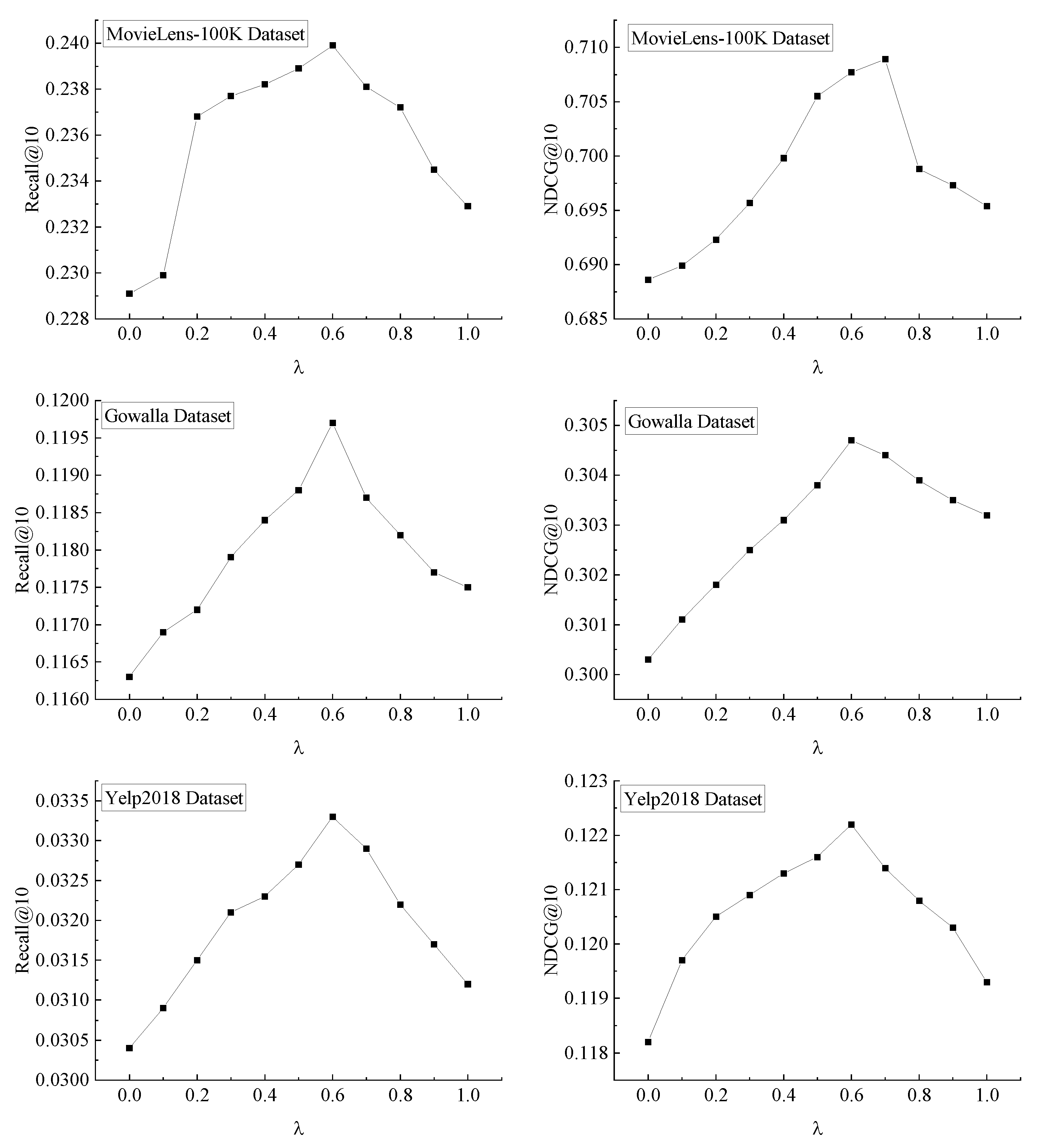
where $\lambda$ is a hyperparameter, which is used to balance the coefficient proportion of the time interval factor and item scoring density factor. $T_d$ represents the time corresponding to the user’s last item rating, $N_{T_i-T_0}$ represents the number of item ratings given by the user received during the time period from $T_0$ to $T_i$, and $N_{T_d-T_0}$ represents the total number of item ratings the user received during the use of the recommendation system.

We add a density factor of the item score in $TF2$ to make the time factor expression more reasonable and record function $f_3\left(t\right)$ as function $f\left(t\right)$.

3.5. Interactive Prediction

This section continues the specific calculation method for interactive prediction in DCCF and introduces time factors to further modify the scoring prediction expression. By updating the feature processes of the local convolutional channel and the global convolutional channel, the local and global features of the nodes are obtained, respectively. The final vector expression of the nodes is obtained by adding the two parts of information.

$$x_u^F=x_u^{local}+x_u^{global}$$

(24)

$$x_i^F=x_i^{local}+x_i^{global}$$

(25)

At this point, by inner product $x_u^F$ and $x_i^F$, user $u$’s rating for item $i$ is obtained.

$$y_{DCFECF}\left(u,i\right)={\left(x_u^F\right)}^T{x}_i^F$$

(26)

Meanwhile, due to the introduction of the time factor, the scoring prediction expression has been further modified, and the final user $u$’s rating for item $i$ is shown in Equation (27).

$${\widehat{y}}_{DCFECF}\left(u,i\right)=y_{DCFECF}\left(u,i\right)·f\left(t\right)={\left(x_u^F\right)}^T{x}_i^F·f\left(t\right)$$

(27)

3.6. Model Optimization

The model training process uses the paired BPR loss function to optimize parameters and trains in a way that maximizes the gap between positive samples and negative samples:

$$los{s}_{BPR}={\displaystyle \sum _{\left(u,i,j\in o\right)}- ln\sigma \left({\widehat{y}}_{ui}-{\widehat{y}}_{uj}\right)}$$

(28)

$\mathrm{O}=\{\left(u,i,j\right)|\left(u,i\right)\in {\mathrm{O}}^{+},\left(u,j\right)\in {\mathrm{O}}^{-}\}$ represents training data, which includes both positive and negative samples in a 1:1 ratio. Each historical interaction record between users and different items in the training set is treated as a positive sample, while negative samples are randomly selected from each user item set that has not had any interaction. $\mathsf{\sigma }(\cdot )$ is the sigmoid activation function and uses the Adam optimizer to update and optimize parameters.

4. Evaluation and Analysis

4.1. Experimental Setup

4.1.1. Experimental Dataset

We selected three publicly available datasets commonly used to evaluate recommendation algorithms for the experiments. In each dataset, select 80% as the training set and the remaining 20% as the test set. The dataset information is shown in

Table 1. Description of the datasets.

Datasets	Number of Users	Number of Items	Number of Interactions
MovieLens-100K	943	1682	100,000
Gowalla	29,858	40,981	1,027,370
Yelp2018	31,668	38,048	1,561,406

.

4.1.2. Contrast Model

We selected four different network structures models, GC-MC, NGCF, LR-GCCF, and DCCF, as performance references for comparative experiments.

GC-MC: Transforms the historical interaction records between users and items into a bipartite graph format and uses a single-layer graph convolutional network to obtain vector representations of users and items.

NGCF: Using multi-layer graph convolutional networks to expand locally, obtain higher-order information, and update vector representations of users and items.

LR-GCCF: Improvements have been made to the NGCF model, simplifying model design and removing some components that affect recommendation performance.

DCCF: Introduce a transition matrix and set a transition probability threshold to determine the neighborhood range of nodes, use a single-layer network structure to complete the calculation, and use K-means clustering to construct a global interaction graph.

4.1.3. Evaluation Index

We select two commonly used indicators for evaluating recommendation algorithms: normalized discounted cumulative gain (NDCG@K) and recall (Recall@K), where @K represents K different items in the recommended list returned by the model when evaluating the results. Generally, K is between 10 and 20. In these experiments, we set K = 10.

NDCG@K evaluates the ranking of the recommendation list obtained by the model. The following is the calculation rule: in the recommendation list, the higher the correlation between candidate items and the current user, the higher the evaluation score. The calculation method is shown in Equations (29) and (30).

$$\mathrm{DCG}@\mathrm{K}={\displaystyle \sum _{i=1}^{\mathrm{K}}\frac{r\left(i\right)}{{\log }_2\left(i+1\right)}}$$

(29)

$$\mathrm{NDCG}@\mathrm{K}=\frac{\mathrm{DCG}@\mathrm{K}}{\mathrm{IDCG}@\mathrm{K}}$$

(30)

where $i$ is the position number in the recommendation list. $r\left(i\right)$ represents the score of the item in the $i$-th position. DCG@K is the total score of the candidate items in the current recommendation list considering the sorting order factor. IDCG@K is the normalization parameter, representing the maximum value that DCG@K can achieve.

Recall@K is the recall index of a recommendation list, which represents the correct proportion of model predictions in real-world interactions. The calculation method is shown in Equation (31):

$$\mathrm{Recall}@\mathrm{K}=\frac{\mathrm{TP}}{\mathrm{TP}+\mathrm{FN}}$$

(31)

where TP represents the number of positive samples predicted as positive samples in the recommendation model, and FN represents the number of positive samples predicted as negative samples in the recommendation model.

4.1.4. Experimental Environment and Parameter Settings

Experimental configuration: the graphics card is RTX2080TI; the processor is Intel (R) Xeon (R) Bronze 3104; memory is 32 GB; the operating system is Windows 10 LTSC; the model is coded based on the deep-learning framework PyTorch 1.7.0; the programming language is Python.

The paired BPR loss function is used to optimize all models in the experiment. In terms of parameter settings, the training batch size is fixed at 1024. In the global convolutional channel, it is necessary to construct the global interaction graph through clustering. Due to differences in the size of the three datasets, the number of clusters on the three datasets is set to {20, 100, 100}, and the learning rate is selected from {0.0001, 0.0005, 0.001, 0.005}. The hyperparameter, which has a great impact on the performance of the model, adopts the way of setting corresponding hyperparameter sensitivity experiments to verify its reasonable value: in the local convolution channel, experiments are carried out when the highest neighborhood order is {1, 2, 3, 4}, respectively; in the global convolutional channel, the number of neighboring nodes is selected in {10, 20, 30, 40, 50}; in the time factor expression, parameters $\lambda$ are selected in {0, 0.1, 0.2, 0.3, 0.4, 0.5, 0.6, 0.7, 0.8, 0.9, 1.0}.

4.2. Experimental Analysis

4.2.1. Sensitivity Experiment of Hyperparameter

(1)

The Highest Neighborhood Order in Local Convolutional Channels

We set the number of neighboring nodes in the global convolutional channel to 20 and the parameter $\lambda$ value to 0.6. By adjusting the highest neighborhood order in the local convolutional channel, we conducted experiments on three sets of datasets based on evaluation indicators Recall@10 and NDCG@10. The experimental results are shown in Figure 3.

From Figure 3, it can be seen that the performance of the model gradually improves with the increase in neighborhood order. Except for the MovieLens-100K dataset, it performs best when the highest neighborhood order is three. Therefore, the highest neighborhood order of the local convolutional channel is set to three.

(2)

The Number of Neighboring Nodes in Global Convolutional Channels

We set the highest neighborhood order of the local convolutional channel to three and the parameter $\lambda$ value to 0.6. We conducted experiments by adjusting the number of neighboring nodes in the global neighborhood of the global convolutional channel. The experimental results are shown in Figure 4.

From Figure 4, it can be seen that on the three datasets, the DCFECF model has the best performance for the evaluation indicators Recall@10 when the number of neighboring nodes is 40, 30, and 30, respectively; for evaluation indicators NDCG@10, the best performance is achieved when the values are 40, 20, and 30, respectively. It can be seen that the model performs better when the number of neighboring nodes in the global neighborhood is around 30. Excessive neighborhood expansion may extract unnecessary node information. Therefore, the number of neighboring nodes in the global convolutional channel is set to 30.

(3)

The Value of Parameter $\lambda$ in the Time Factor Expression

We set the highest neighborhood order of the local convolutional channel to 3 and the number of neighboring nodes in the global convolutional channel to 30. We adjusted the value of parameter $\lambda$ in the time factor expression, and the experimental results are shown in Figure 5.

From Figure 5, it can be seen that on the three datasets, the DCFECF model exhibits the best performance for the evaluation indicators Recall@10 when parameter $\lambda$ values are 0.6, 0.6, and 0.6, respectively; for evaluation indicators NDCG@10, the best performance is achieved when $\lambda$ values are 0.7, 0.6, and 0.6, respectively. It can be seen that when the parameter $\lambda$ value is around 0.6, the DCFECF model performs better. In addition, the performance of the model is greater when the value of parameter $\lambda$ is 1 than when the value is 0. From Equation (23), it can be seen that when $\lambda$ is set to 1, only the time interval factor is considered, and when $\lambda$ is set to 0, only the rating item density factor is considered. This indicates that when only one factor is considered, the time interval factor has a greater impact on the user’s memory level, while the rating item density factor has a smaller impact on the user’s memory level. When the value of $\lambda$ is around 0.6, the coefficient ratio of the time interval factor is higher, while the coefficient ratio of scoring item density factor is lower, which is consistent with the experimental results that the time interval factor has a significant impact on users’ memory level. By taking an appropriate value for parameter $\lambda$ and balancing the coefficient ratio of the two factors, the filtering effect of the time factor on the model prediction results can be better. This indicates that it is reasonable to consider both the time interval factor and the density factor of scoring items and set parameter $\lambda$ to balance the proportion of the two factors.

4.2.2. Comparative Experiment

Figure 6 shows the results of comparative experiments conducted on three datasets using Recall@10 and NDCG@10 as evaluation indicators. DCFECF performed the best on all three datasets, and among the four benchmark comparison models, the DCCF model performed the best. The NGCF model uses a multi-layer graph convolutional network to aggregate higher-order neighborhood information in the local structure, which consistently performs better than the GC-MC model using a single-layer graph convolutional network. The LR-GCCF model is simplified on the basis of the NGCF model. The activation function and parameter matrix are removed, and the model performance is improved. Both DCFECF model and DCCF model use the single-layer graph convolution network to calculate, suppress the over-smoothing problem, effectively filter neighborhood information, and use clustering to construct global interaction graph, which overcomes the problem that interaction information is limited to the local neighborhood, and has better performance than NGCF model, GC-MC model, and LR-GCCF model. Compared to the DCCF model, the DCFECF model achieved a maximum improvement of 2.3% and 4.1% on three datasets based on two evaluation indicators, indicating that improvements to the DCCF model can further improve the algorithm recommendation performance.

4.2.3. Ablation Experiment

(1)

The Ablation Experiment on the Method of Calculating Transfer Probability Threshold

We deconstruct the structure of the DCFECF model, which only preserves the method of obtaining the transition probability threshold. We use the K-means clustering algorithm in the DCCF model to construct a global interaction graph without introducing time factors. The model with this structure is called DCFECF_1. The transition probability threshold in the DCCF model is still set at 0.5. The experimental results based on evaluation indicators Recall@10 and NDCG@10 on three datasets are shown in

Table 2. Recall@10 performance under the method of calculating transfer probability threshold.

Model	Recall@10
	MovieLens-100K	Gowalla	Yelp2018
DCCF	0.2328	0.1142	0.0315
DCFECF_1	0.2360	0.1168	0.0321

and

Table 3. NDCG@10 performance under the method of calculating transfer probability threshold.

Model	NDCG@10
	MovieLens-100K	Gowalla	Yelp2018
DCCF	0.6907	0.2939	0.1176
DCFECF_1	0.6997	0.3013	0.1202

.

From these tables, it can be seen that the performance of the DCFECF_1 model with the introduction of the transition probability threshold calculation method is always better than that of the DCCF model. This indicates that the transition probability threshold calculation method proposed in the DCFECF model can obtain different order transition probability thresholds based on data samples. Compared with the fixed transition probability threshold set in the DCCF model, it is more in line with practical application scenarios and can filter neighborhood information more effectively.

(2)

The Ablation Experiment of Clustering Algorithm

We deconstruct the structure of the DCFECF model by not using the method of obtaining the transition probability threshold (which is a fixed value and still set to 0.5) and do not introduce a time factor. For clustering algorithms, we name the model that only uses the K-means++ clustering algorithm DCFECF_2. The model that only uses the fuzzy C-means clustering algorithm is DCFECF_3. The model using the fuzzy C-means clustering algorithm optimized based on the K-means++ clustering algorithm is DCFECF_4. The experimental results based on evaluation indicators Recall@10 and NDCG@10 on three datasets are shown in

Table 4. Recall@10 performance under introducing different clustering algorithms.

Model	Recall@10
	MovieLens-100K	Gowalla	Yelp2018
DCCF	0.2326	0.1144	0.0315
DCFECF_2	0.2339	0.1156	0.0318
DCFECF_3	0.2341	0.1155	0.0319
DCFECF_4	0.2364	0.1171	0.0322

and

Table 5. NDCG@10 performance under introducing different clustering algorithms.

Model	NDCG@10
	MovieLens-100K	Gowalla	Yelp2018
DCCF	0.6917	0.2938	0.1175
DCFECF_2	0.6951	0.2970	0.1189
DCFECF_3	0.6954	0.2968	0.1192
DCFECF_4	0.7001	0.3021	0.1204

.

From these tables, it can be seen that because the K-means++ clustering algorithm is an improvement on the K-means clustering algorithm, the performance of DCFECF_2 is always better than DCCF. Compared to the K-means clustering algorithm, the fuzzy C-means clustering algorithm integrates the essence of fuzzy theory and can provide more flexible clustering results, so the performance of DCFECF_3 is always better than DCCF. DCFECF_4 uses the K-means++ clustering algorithm to determine the initial clustering center of the fuzzy C-means clustering algorithm and then uses the fuzzy C-means clustering algorithm for clustering, which can achieve better clustering performance compared to other models. Therefore, it always has the best performance compared to other models, indicating that the clustering algorithm proposed in DCFECF has better clustering performance than the K-means clustering algorithm. The spatial complexity of the K-means clustering algorithm is O(d(N + M + K)), while the spatial complexity of the fuzzy C-means clustering algorithm optimized based on the K-means++ clustering algorithm is O(d(N + M)K), where d is the vector embedding dimension, N + M is the total number of nodes, and K is the number of clusters. In practical large-scale data scenarios, N + M is usually much larger than K, indicating that the improved clustering effect also increases some spatial overhead.

(3)

The Ablation Experiment of the Time Factor

We deconstruct the structure of the DCFECF model by not using the method of obtaining the transition probability threshold but only using the K-means clustering algorithm to construct a global interaction graph and introducing a time factor. The model that introduces the time factor $TF1$ is the DCFECF1 model, the model that introduces the time factor $TF2$ is DCFECF2, and the model that introduces the time factor $TF3$ is DCFECF3. The experimental results are shown in

Table 6. Recall@10 performance under introducing the time factor.

Model	Recall@10
	MovieLens-100K	Gowalla	Yelp2018
DCCF	0.2325	0.1141	0.0314
DCFECF1	0.2338	0.1146	0.0316
DCFECF2	0.2344	0.1155	0.0320
DCFECF3	0.2366	0.1173	0.0324

and

Table 7. NDCG@10 performance under introducing the time factor.

Model	NDCG@10
	MovieLens-100K	Gowalla	Yelp2018
DCCF	0.6910	0.2936	0.1173
DCFECF1	0.6931	0.2949	0.1178
DCFECF2	0.6948	0.2971	0.1189
DCFECF3	0.7004	0.3019	0.1206

.

From these tables, it can be seen that the DCFECF model has better performance than the DCCF model, indicating that introducing a time factor can improve the predictive ability of the model. In addition, among the three DCFECF models that introduced time factors, the DCFECF3 model achieved the best performance on all three datasets, indicating that the improvement of the time factor expression in this paper is effective, and it is reasonable to consider adding the item scoring density factor to the time factor, which can further improve the predictive ability of the model.

5. Conclusions

This paper proposes a dual-channel feature enhanced collaborative filtering recommendation algorithm (DCFECF) to solve the problem that in the DCCF model, the fixed threshold of transition probability leads to a decrease in the filtering effect of neighborhood information, the K-means clustering algorithm tends to make the clustering results fall into local optimization, resulting in incomplete global interaction graph, and does not consider the impact of time factors on the prediction results. In the local convolutional channel, transforming the transition probability threshold from a fixed value to a dynamic value can better filter neighborhood information and improve the predictive ability of the model; in the global convolutional channel, the K-means++ clustering algorithm is first used to determine the clustering center, and then the fuzzy C-means clustering algorithm is used to solve the local optimal problem, which can construct a more comprehensive global interaction graph, simultaneously introducing the time factor to further modify the predicted results; through experiments, the rationality and effectiveness of the DCFECF model in improving the DCCF model were verified.

In future research, we will focus on two aspects, namely the expression of interaction relationships between nodes and the construction of interaction graphs to modify the DCFECF model. We will modify the attention mechanism [19], adaptively learn and fuse weights, and further express the interaction relationships between nodes after determining their neighborhood range, thereby improving recommendation performance. In addition, we will design different custom rules to construct interaction diagrams [20], combine different information, and construct more comprehensive global interaction diagrams, making the model more interpretable.

References

1. Zhu, Z.G.; Li, W.Y.; Jiang, P.; Zhou, P. Survey of graph neural networks in session recommender systems. Comput. Eng. Appl. 2023, 59, 55–69. [Google Scholar]
2. Wu, Z.H.; Pan, S.R.; Chen, F.W.; Long, G.D.; Zhang, C.Q.; Yu, P.S. A Comprehensive Survey on Graph Neural Networks. IEEE Trans. Neural Netw. Learn. Syst. 2020, 32, 4–24. [Google Scholar] [CrossRef] [PubMed] [Green Version]
3. Zhou, J.; Cui, G.Q.; Hu, S.D.; Zhang, Z.Y.; Yang, C.; Liu, Z.Y.; Wang, L.F.; Li, C.C.; Sun, M.S. Graph neural networks: A review of methods and applications. AI Open 2020, 1, 57–81. [Google Scholar] [CrossRef]
4. Li, Q.M.; Han, Z.H.; Wu, X.M. Deeper insights into graph convolutional networks for semi-supervised learning. In Proceedings of the AAAI Conference on Artificial Intelligence, New Orleans, LA, USA, 2–7 February 2018; Volume 32, pp. 3538–3545. [Google Scholar]
5. Huang, W.B.; Rong, Y.; Xu, T.Y.; Sun, F.C.; Huang, J.Z. Tackling over-smoothing for general graph convolutional networks. arXiv, 2020; arXiv:2008.09864. [Google Scholar]
6. Wang, X.; Wang, R.J.; Shi, C.; Song, G.J.; Li, Q.Y. Multi-component graph convolutional collaborative filtering. In Proceedings of the AAAI Conference on Artificial Intelligence, New York, NY, USA, 7–12 February 2020; Volume 34, pp. 6267–6274. [Google Scholar]
7. Miao, Y.X.; Song, C.H.; Niu, B.N.; Kang, R.X. Dual-Channel Graph Collaborative Filtering Recommendation Algorithm. Comput. Eng. 2022, 48, 121–128. [Google Scholar] [CrossRef]
8. Berg, R.V.D.; Kipf, T.N.; Welling, M. Graph convolutional matrix completion. In Proceedings of the 24th ACM SIGKDD International Conference on Knowledge Discovery & Data Mining, London, UK, 19–23 August 2018. [Google Scholar]
9. Wang, X.; He, X.N.; Wang, M.; Feng, F.L.; Chua, T.S. Neural graph collaborative filtering. In Proceedings of the 42nd International ACM SIGIR Conference on Research and Development in Information Retrieval, Paris, France, 21–25 July 2019; pp. 165–174. [Google Scholar]
10. Chen, L.; Wu, L.; Hong, R.C.; Wang, M. Revisiting graph based collaborative filtering: A linear residual graph convolutional network approach. In Proceedings of the AAAI Conference on Artificial Intelligence, New York, NY, USA, 7–12 February 2020; Volume 34, pp. 27–34. [Google Scholar]
11. Ji, S.Y.; Feng, Y.F.; Ji, R.R.; Zhao, X.B.; Tang, W.W.; Gao, Y. Dual Channel Hypergraph Collaborative Filtering. In Proceedings of the 26th ACM SIGKDD International Conference on Knowledge Discovery & Data Mining, Virtual, 6–10 July 2020; pp. 2020–2029. [Google Scholar]
12. Hassan, N.S.; Abdulazeez, A.M.; Zeebaree, D.Q.; Hasan, D.A. Medical images breast cancer segmentation based on k-means clustering algorithm: A review. Asian J. Res. Comput. Sci. 2021, 9, 23–38. [Google Scholar] [CrossRef]
13. Xie, Z.Z. Personalized Recommendation Method Based on User Rating and Category Clustering. Master’s Thesis, Tianjin University of Commerce, Tianjin, China, 2021. [Google Scholar]
14. Hechtlinger, Y.; Chakravarti, P.; Qin, J.N. A generalization of convolutional neural networks to graph-structured data. arXiv 2017, arXiv:1704.08165. [Google Scholar]
15. Yin, B.J.; Zuo, R.G.; Sun, S.Q. Mineral prospectivity mapping using deep self-attention model. Nat. Resour. Res. 2022, 32, 37–56. [Google Scholar] [CrossRef]
16. Wang, Y.G.; Liu, K.Q. Collaborative Filtering Recommendation Algorithm for Clustering Optimization. Comput. Eng. Appl. 2020, 56, 66–73. [Google Scholar]
17. Yan, H.C.; Wang, Z.R.; Li, W.F.; Gu, J.T. Time-Based Fuzzy Cluster Collaborative Filtering Recommendation Algorithm. Comput. Eng. Sci. 2021, 43, 2084–2090. [Google Scholar]
18. Zhang, Q.S.; Zhu, M. Collaborative Filtering Algorithm Combining Time-Weighted Trust and User Preferences. Comput. Eng. Appl. 2022, 58, 112–118. [Google Scholar]
19. Fan, Z.W.; Liu, Z.W.; Zhang, J.W.; Xiong, Y.; Zheng, L.; Yu, P.S. Continuous-Time Sequential Recommendation with Temporal Graph Collaborative Transformer. In Proceedings of the 30th ACM International Conference on Information & Knowledge Management, Virtual, 1–5 November 2021; pp. 433–442. [Google Scholar]
20. Liu, Z.W.; Meng, L.; Jiang, F.; Zhang, J.W.; Yu, P.S. Deoscillated Adaptive Graph Collaborative Filtering. Proceedings of Topological, Algebraic, and Geometric Learning Workshops, Virtual, 29 April 2022; Volume 196, pp. 248–257. [Google Scholar]
Figure 1. The prediction process of DCFECF.
Futureinternet 15 00215 g001
Figure 2. The model framework of DCFECF.
Futureinternet 15 00215 g002
Figure 3. Model performance under different neighborhood orders.
Futureinternet 15 00215 g003
Figure 4. Model performance under different numbers of neighboring nodes in the global neighborhood.
Futureinternet 15 00215 g004
Figure 5. Model performance under different values of λ in the time factor expression.
Futureinternet 15 00215 g005
Figure 6. Comparative experiment results.
Futureinternet 15 00215 g006