Abstract
This study, focusing on identifying rare attacks in imbalanced network intrusion datasets, explored the effect of using different ratios of oversampled to undersampled data for binary classification. Two designs were compared: random undersampling before splitting the training and testing data and random undersampling after splitting the training and testing data. This study also examines how oversampling/undersampling ratios affect random forest classification rates in datasets with minority dataor rare attacks. The results suggest that random undersampling before splitting gives better classification rates; however, random undersampling after oversampling with BSMOTE allows for the use of lower ratios of oversampled data.
1. Introduction
The internet generates traffic at a rate of 6.59 billion GB per second [1]. Approximately 1–3% of this traffic is malicious [2]. Advances in machine learning (ML) have allowed us to detect some of these attacks but not all. The challenge that cyber security experts face is not one of having enough data but one of having enough of the right type of data. Some organizations never see anomalous data on their network; most network traffic is generated by routine workplace business. Given this scenario, it is hard to know what to look for since we have such a small sample size of the attacks. Some types of attacks are more frequent than others, and it is only in the infrequent or rare attacks, or minority data, that this detection problem lies. Machine learning models, by their very nature, are good at detecting patterns where there is more data (in majority data); hence, detection of rare attacks (minority data) is challenging for machine learning models.
Minority data is a tiny percentage of network intrusion datasets, and for the purposes of this work, we are defining minority data as less than 0.1%. Various oversampling techniques, including different smote methods, random oversampling, ADASYN, and others, have been used by researchers to try to model minority data better. Oftentimes a combination of oversampling (of minority data) and undersampling (of majority data) is used [3].
When oversampling and undersampling are used, researchers have to determine how much undersampling should occur, how much oversampling should occur, and when the resampling should occur in the process. This research presents two different design methodologies, one performing random undersampling before splitting the training and testing data and the second performing random undersampling after splitting the training and testing data. In addition, for each of these two designs, the paper compares different ratios of random undersampling to oversampling using BSMOTE. Finally, binary classification using random forest is used to classify the various combinations of the data. For this research, two datasets have been used—the first being a widely used network intrusion dataset, UNSW-NB15 [4], and the second being a newly created network intrusion dataset based on the MITRE ATT&CK framework, UWF-ZeekData22 [5].
The rest of this paper is organized as follows. Section 2 presents the background; Section 3 presents works related to oversampling and undersampling; Section 4 explains the datasets used in this study; Section 5 presents the experimental designs; Section 6 presents the hardware and software configurations; Section 7 presents the metrics used for assessment of the classification results; Section 8 presents the results and discussion; Section 9 presents the conclusions; and Section 10 presents the future works.
2. Background
To adequately address resampling, the resampling techniques used in this paper are briefly explained next. Though oversampling and undersampling are aimed at changing the ratios between the minority and majority classes, respectively, this is particularly important when the minority classes are minimal, that is, in the case of rare attacks.
A minority class refers to very low-occurring data categories. In this work, since a binary classification was performed, the dataset for each experimentation contained only two data types—one attack category and benign data. For example, for the analysis of worms, the dataset contained only worms and benign data. Out of these two categories of data, worms would be considered the minority class. Table 1, which presents the UNSW-NB15 dataset, shows that worms account for 0.006% of the data and 0.007% of the benign data. The raw data count for worms is 174 compared to the benign data count of 2,218,761.
Oversampling is the process of generating samples to increase the size of the minority class. Random oversampling involves randomly selecting samples from the minority class, with replacement, and adding them to the dataset [6]. Random oversampling can also lead to overfitting the data [3].
Various oversampling techniques are available, including various types of Synthetic Minority Oversampling Techniques (SMOTE) and ADASYN. SMOTE generates synthetic samples rather than resampling with replacement. These samples are generated along the line segment adjoining k-minority class neighbors [7]. In Borderline SMOTE (BSMOTE), a variant of the original SMOTE, borderline minority samples are identified and then synthetic samples are generated [8].
ADASYN [9] is a pseudo-probabilistic oversampling technique that uses a weighted distribution for different minority data points. This weighted distribution is based on the level of difficulty in learning, and more synthetic data are generated for minority class examples that are harder to learn than minority examples that are easier to learn [10].
Random undersampling samples the majority class by randomly picking samples with or without replacement from the majority class [11]. After random undersampling, the number of cases of the majority class decreases, significantly reducing the model’s training time. However, the removed data points may include significant information leading to a decrease in classification results [3].
3. Related Works
For cybersecurity or network intrusion detection analysis, it is difficult to obtain a good workable dataset; among the few available, most are highly imbalanced due to the nature of the attacks. Certain attacks are rare in the real world, but measures must be taken to safeguard against them. The rarer the attack, the lesser the chance of it getting detected by a machine learning model.
Oversampling and undersampling are standard methods used by researchers to tackle class imbalance problems [3,7,12]. Oversampling generates synthetic samples from the existing minority class to balance the data or to have more instances for the classifier. Undersampling, on the other hand, reduces the majority class instances to bring the imbalance scale to normalcy. Though both these methods have inherent advantages and disadvantages, they can be used separately or combined with balancing ratios. It is possible to selectively downsize only negative examples and keep all positive examples in the training set [13]. A major disadvantage of undersampling is the loss of data, and hence possibly critical information.
Oversampling increases the training time due to an increase in the training set [12], and may overfit the model [14]. Ref. [14] found that oversampling minority data before partitioning resulted in 40% to 50% AUC score improvement. When the minority oversampling is applied after the split, the actual AUC improvement is 4% to 10%. This behavior is due to what is termed as data leakage, caused by generating training samples correlated with the original data points that end up in the testing set [14]. Ref. [15] found that the synthetic instance creation approach plays a more significant role than the minority instance selection approach. The critical difference between these two papers is that the first process creates instances along the line connecting the two minority instances, while the second approach creates synthetic minority samples in the bounding rectangle created by joining the two minority instances.
Hence, both oversampling and undersampling can have potential overfitting or underfitting, respectively. Studies have been carried out with various combinations of oversampling and undersampling [12,16,17]. Random undersampling was also combined with each oversampling technique—SMOTE, ADASYN, Borderline, SVM-SMOTE, and random oversampling in [18]. Various percentages were used from each of these techniques to study the effect on minority class predictions. The results of each combination are highly dependent on the domain and distribution of the dataset [19]. In one domain, undersampling might help more than oversampling, but in another domain, it may be vice versa.
Some researchers have combined synthetic oversampling with other techniques, such as Grid Search (GS), to improve the prediction of attack traffic [20].
While the above papers present novel ways to examine the class imbalance classification problem, none directly addresses the problem of identifying rare attacks using different ratios of the sampling methods. The novelty of this research is that it considers different ratios of majority data to minority data when identifying rare attacks. Additionally, two different designs are compared—random undersampling before splitting the data and random undersampling after splitting the data, with different oversampling ratios.
4. The Datasets
Two datasets were used in this study: (i) a well-known network intrusion dataset, UNSW-NB15 [4] and (ii) a new network intrusion dataset created based on the MITRE ATT&CK framework, UWF-ZeekData22 [21].
4.1. UNSW-NB15
UNSW-NB15 [4], published in 2015, is a hybrid of real-world network data and simulated network attacks, comprising 49 features and 2.5 million rows. There are 2.2 million rows of normal or benign traffic, and the other 300,000 rows comprise nine different modern attack categories: Fuzzers, Reconnaissance, Shellcode, Analysis, Backdoors, DOS, Exploits, Worms, and Generic. Some attack categories, such as Worms, Shellcode, and Backdoors, that comprised only 0.006%, 0.059%, and 0.091%, of the total traffic, respectively, can be considered rare attacks. These are the three attack categories of particular interest in this research, and the rare attacks will be considered the minority classes. Table 1 presents the distribution of the attack families in this dataset, ordered from the smallest category to the largest category.

Table 1.
UNSW-NB15: distribution of attack families [4].
4.2. UWF-ZeekData22
UWF-ZeekData22 [5,21], published in 2022, is developed from data collected from Zeek, an open-source network-monitoring tool, and labeled based on the MITRE Adversarial Tactics, Techniques, and Common Knowledge (ATT&CK) framework. This dataset has approximately 9.280 million attack records and 9.281 benign records [22]. The breakdown of the data, that is, the percent of attack data for each attack type, is presented in Table 2, ordered from the smallest category to the largest category. For this analysis, two rare tactics were used: Privilege_escalation and Credential_access. Privilege_escalation and Credential_access form 0.00007% and 0.00016% of the total network traffic, respectively, and hence can be classified as rare attacks. These rare attacks will be treated as the minority classes.
Table 2.
UWF-ZeekData22: distribution of MITRE ATT&CK tactics [5,21].
5. Experimental Design
The experimental design compares two approaches to solve the problem of having significantly small samples of minority data: (a) resampling or random undersampling before a stratified split (Figure 1a) and (b) resampling or random undersampling after a stratified split (Figure 1b). Since the objective of this work is to identify minority data or rare attacks, stratified sampling was used to guarantee that the training and testing data included minority data. However, the question is, when is it best to perform stratified sampling? In stratified sampling, the data are divided into groups and a certain percentage of samples are taken randomly from each group. This guarantees that there will be samples from the minority class in the data. For the purposes of this study, significantly small minority data are defined as <0.1 % of the total sample.
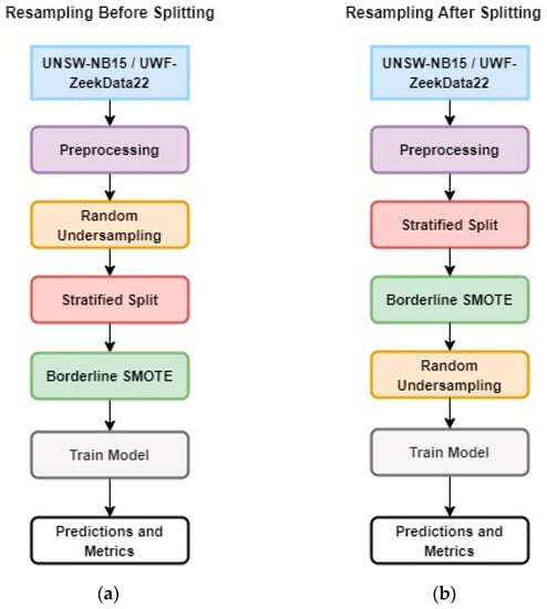
Figure 1.
Experimental design: (a) Resampling Before Splitting; (b) Resampling After Splitting.
Basically, the two approaches differ in the preprocessing sequence prior to the machine learning model execution and have different approaches to creating training and testing data. In the first design, resampling before splitting, the data are preprocessed, and then random undersampling is performed. This is followed by a stratified split and oversampling using borderline SMOTE (B-SMOTE). Finally, these data were used for training and testing the machine learning model using random forest.
In the second design, resampling after splitting, after the initial preprocessing steps, the data are split (using stratified sampling). This method retains the stratified ratio of the majority to minority class since the stratified split was performed on the whole data. This is followed by oversampling using BSMOTE and random undersampling. Finally, these data were used to train and test the machine learning model using random forest.
5.1. The Classifier Used: Random Forest
Random forest (RF) is a highly used machine learning classifier that is basically an ensemble way of classifying records. In the RF algorithm, the decision of multiple decision trees taken together is used to come up with the final classification label [23].
The RF algorithm works by first generating each decision tree by randomly selecting a bootstrap sample. A bootstrap sample is a randomly selected sample from a dataset with replacement [24]. Each decision tree is trained with a separate bootstrap sample. Hence, if a random forest has N trees, N bootstrap samples will be required. Randomization is introduced during tree training. Features are randomly selected when a decision tree node splits, and of the randomly selected features, the best feature is selected based on statistical measures, such as information gain and Gini index [24]. Once forest training is complete, N-trained decision trees are created. A classification is made on one or more samples. RF classifies samples by querying each decision tree with the sample. A tally is kept to aggregate all classifications made by the decision trees [24]. Once all trees have voted with a classification, the label with the most votes is chosen. Hence, RF is basically an ensemble technique based on decision trees.
5.2. Preprocessing
With regard to preprocessing, each dataset was handled differently, but information gain was used on both datasets to identify the relevant features. First, the information gain algorithm is explained, and then the preprocessing performed in each dataset is presented.
5.2.1. Information Gain
Information gain (IG) is used to assess the relative relevance of features in a dataset and is useful for classification. Information gain is calculated by removing the randomness in the dataset, which is measured by a class’s entropy [23].
The following calculations were performed on each feature to produce information gain values for ranking purposes [23].
where
where:
- Info(D) is the average amount of information needed to identify the class level of a tuple in the data, D;
- InfoA(D) is the expected information required to classify a tuple from D based on the partitioning by attribute A;
- pi is the nonzero probability that an arbitrary tuple belongs to a class;
- |Dj|/|D| is the weight of the jth partition;
- V is the number of distinct values in attribute A.
5.2.2. Preprocessing UNSW-NB15
For preprocessing UNSW-NB15, first, the following columns were dropped:
- ct_flw_http_mthd and is_ftp_login;
- Unique identifiers and time stamps;
- IP addresses.
Other preprocessing that was performed:
- The attack categories, NaN, were filled with zeros;
- Categorical data were turned into numeric representation: protocol, state, and attack category;
- A normalization technique was used on continuous data for all numeric variables:
Finally, IG was calculated on the remaining columns of this dataset, and columns with low information gain were not used. Columns dropped due to low information gain were service, dloss, stepd, dtcpb, res_bdy_len, trans_depth, and is_sm_ips_ports.
5.2.3. Preprocessing UWF-ZeekData22
For UWF-ZeekData22, the following preprocessing was performed following [22]:
- Continuous features, duration, orig_bytes, orig_pkts, orig_ip_bytes, resp_bytes, resp_pkts, resp_ip_bytes, and missed_bytes were binned using a moving mean;
- Nominal features, that is, features that contain non-numeric data, were converted to numbers using the StringIndexer method from MLib [25], Apache Spark’s scalable machine learning library. The nominal features in this dataset were proto, conn_state, local_orig, history, and service;
- The IP address columns were categorized using the commonly recognized network classifications [26];
- Port numbers were binned as per the Internet Assigned Numbers Authority (IANA) [27].
Following the binning, IG was calculated on the binned dataset. Attributes with low IG were removed and not used for classification.
6. Hardware and Software Configurations
Table 3 and Table 4 present the hardware and software configurations and python libraries, respectively, used in this research.
Table 3.
Hardware and software configurations.
Table 4.
Python library versions.
6.1. Hardware and Software Used in Random Undersampling before Stratified Splitting
Random undersampling before stratified splitting simulations was run on an x64-based processor with a 64-bit operating system. This Windows Home machine was running version 22H2 build 22621.819 and had an AMD Ryzen 7 5700 with 32 GB of RAM and an RTX 3060 Video card. CUDA for Python was installed; however, none of the trials used the parallel processing abilities of the machine.
6.2. Python Libraries Used in Random Undersampling before Stratified Splitting
Python version 3.9 was used with Jupyter Notebooks on Anaconda version 2022.10. Packages included pandas 1.5.2, scikit-learn 1.9.3, NumPy 1.23.5, and imblearn 0.10.0. The random forest machine learning algorithm was implemented using the scikit-learn RandomForestRegressor module. Borderline SMOTE was implemented using the BorderlineSMOTE module of the imblearn.over_sampling package.
6.3. Hardware and Software Used in Random Undersampling after Stratified Splitting
Random undersampling after stratified splitting simulations was run on a machine with Windows Home version 21H2 with OS build 22000.1219 run by an Intel Core i7 1165G7 processor and 16 GB RAM.
6.4. Python Libraries Used in Random Undersampling after Stratified Splitting
Python version 3.10.4 was used with Jupyter Notebooks on Anaconda version 2021.05. Packages included pandas 1.5.0, scikit-learn 1.0.2, NumPy 1.23.4, and imblearn 0.0.
6.5. Stratified Sampling
Scikit-learn in Python was used to generate the training and testing stratified splits.
7. Metrics Used for the Assessment of Results
The objective of this research is to show how a combination of undersampling and oversampling techniques helps build a model which classifies minority classes more accurately. Two approaches were taken for preparing the data: random undersampling before splitting and random undersampling after splitting, and different proportions of oversampling were used (from 0.1 to 1.0, incremented at intervals of 0.1), while the undersampling was maintained at a constant of 0.5 (50%).
7.1. Classification Metrics Used
For evaluating the classification of the random forest runs, the following matrices were used: accuracy, precision, recall, F-Score, and macro precision.
Accuracy: Accuracy is the number of correctly classified instances (i.e., True Positives and True Negatives) divided by the total number of instances [28].
Accuracy = [True Positives (TP) + True Negatives (TN)]/[TP + False Positives
+ TN + False Negatives]
+ TN + False Negatives]
Precision: Precision is the proportion of predicted positive cases that are correctly labeled as positive [29]. Precision by label considers only one class and measures the number of times a specific label was predicted correctly, normalized by the number of times that label appears in the output.
Precision = Positive Predictive Value = [True Positives]/[True Positives +
False Positives]
False Positives]
Recall: Recall is the ability of the classifier to find all the positive samples, or the True Positive Rate (TPR). Recall is also known as sensitivity, and is the proportion of Real Positive cases that are correctly predicted as Positive (TP) [29].
- All Real Positives = [True Positives + False Negatives]
- All Real Negatives = [True Negatives + False Positives]
Recall = True Positive Rate = [True Positives]/[All Real Positives]
F-Score: The F-score is the harmonic mean of a prediction’s precision and recall metrics. It is another overall measure of the test’s accuracy [29].
F-Score = 2 ∗ [Precision ∗ Recall]/[Precision + Recall]
Recall, sensitivity, and TPR connate the same measure.
Macro Precision: Macro precision finds the unweighted mean of the precision values. This does not take label imbalance into account [30].
7.2. Welch’s t-Tests
Welch’s t-tests were used to find the differences in the means of the different oversampling percentages. When comparing metrics across two successive percentage runs, the increase or decrease in the metric being evaluated has to be determined, and hence a one-tailed Welch’s t-test was used. Welch’s t-test is calculated using the formula:
where and are sample means of the metrics, s12 and s22 are sample variances, n1 and n2 are sample sizes, and the df is calculated using Satterwaite approximation.
The mean of the individual runs for each metric for one oversampling percentage is compared with another, for example, 0.1 vs. 0.2. If the t-score value is high, there is more difference between the two means. In order to determine whether this difference is significant, the p-value was calculated for each t-score. The significance level was kept at 0.1, making the test more sensitive to results and increasing the significance zone. If the p-value is less than the threshold, then the increase or decrease in the t-score value is significant between the two means.
8. Results and Discussion
This section presents the statistical results, followed by a discussion. Since several oversampling techniques are available, the first step was to perform a study to select an oversampling technique. Then, the results of the random undersampling before stratified splitting are presented, followed by the results of the random undersampling after stratified splitting.
8.1. Selection of an Oversampling Technique
An initial analysis was conducted to determine the best synthetic oversampling technique among a few commonly used oversampling techniques, SMOTE, Borderline SMOTE, and ADASYN.
Traditionally, a 70-30 training-testing split is performed on the data. However, in this case, since the occurrences of the minority class are minimal, there is no guarantee that samples from the minority class will be present in both the training data and the testing data without sample stratification by category. Hence, stratified sampling was used to split the data into a 70-30 training-testing ratio.
From the evaluation metrics shown in Figure 2, it is evident that BSMOTE performs better than the other resampling techniques in terms of precision, F-score, and macro precision. SMOTE and ADASYN had better recall than BSMOTE, but the latter performed better overall.
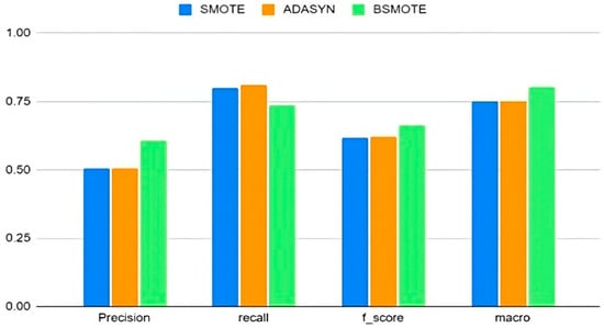
Figure 2.
Comparison of oversampling techniques.
Hence, all future analyses in this work use BSMOTE as the primary oversampling technique, combined with random undersampling. Several researchers have confirmed that neither oversampling nor undersampling alone can successfully classify imbalanced datasets [12,19], let alone identify rare attacks. Hence, this study looks at the effects of varying oversampling percentages.
8.2. Resampling before and after Splitting
For random undersampling before stratified splitting, as well as random undersampling after stratified splitting, the percent of undersampling was kept at 0.5 (50%) and the percent of oversampling varied from 0.1 (10%) of the data to 1.0 (100%) of the data, at increments of 0.1 (10%). That is, 50% of the instances were selected at random from the majority class, and from the minority class, first 0.1 (10%) oversampling was used, then 0.2 (20%), then 0.3 (30%), and so on, until 1.0 (100%).
For UNSW-NB15, the three most minor attack categories, Worms, Shellcode, and Backdoors, were used. Worms, Shellcode, and Backdoors comprise 0.006%, 0.059%, and 0.091% of the total data, respectively. For UWF-ZeekData22, two tactics were used: credential access and privilege escalation. Privilege escalation and credential access were contained in 0.00007 and 0.00016% of the total data respectively.
For each of the attack categories, for random undersampling before stratified splitting, as well as random undersampling after stratified splitting, an average of ten runs were performed. Values are presented for accuracy, precision, recall, F-score, and macro precision for random undersampling of the majority data at 0.5 (50%), and oversampling the minority data using BSMOTE varied from 0.1 (10%) to 1.0 (100%), at increments of 0.1 (10%). The standard deviations (SDs) are also presented. Since only binary classification is performed in this study, the majority of the data were the benign or non-attack data and the minority of the data were the respective attack category, for example, worms or credential access.
8.2.1. Random Undersampling before Stratified Splitting
Table 5 presents the classification results for Random Undersampling Before Stratified Splitting for Worms (UNSW-NB15) for the various oversampling percentages (0.1 to 1.0, at intervals of 0.1). The best results are highlighted in green.
Table 5.
UNSW-NB15: Worms—classification results for random undersampling before splitting.
To determine the best results among the various oversampling percentages, Welch’s t-tests were performed. Results of Welch’s t-tests for UNSW-NB15, Worms Random Sampling before Stratified Splitting (Table 5), are presented in Table 6. The results presented in Table 6 show the t-test comparisons between the results of various oversampling runs. In the first row of comparison between 0.1 and 0.2, we observed that the p-values across all metrics are above 0.1, the significance level. Hence, there is no statistical difference between the compared results. However, in the second row of comparison between 0.1 and 0.3, the recall and F-score had significant differences, and both the t-score values were positive. This implies that 10% oversampling performed better than 30%.
Table 6.
Welch’s t-test results: UNSW-NB15: Worms—random undersampling before splitting.
Hence, based on the analysis in Table 6, the best results were obtained at 0.5 oversampling for Worms (highlighted in green in Table 5). There are, however, sampling ratios that are statistically equivalent to using 0.5, as shown in Table 6. However, an oversampling of 0.5 was chosen as the best since it has the smallest amount of oversampled data and thus would take the least computational time.
Table 7 presents the classification results for Random Undersampling Before Splitting for Shellcode (UNSW-NB15) for the various oversampling percentages (0.1 to 1.0, at intervals of 0.1). The best results are highlighted in green.
Table 7.
UNSW-NB15: Shellcode—classification results for random undersampling before splitting.
Results of Welch’s t-tests for UNSW-NB15 Shellcode Random Undersampling before Splitting (Table 7) are presented in Table 8. Based on the analysis in Table 8, the best results were obtained at 0.4 oversampling for Shellcode (highlighted in green in Table 7).
Table 8.
Welch’s t-test results: UNSW-NB15: Shellcode—random undersampling before splitting.
Table 9 presents the classification results for Random Undersampling Before Splitting for Backdoors (UNSW-NB15) for the various oversampling percentages (0.1 to 1.0, at intervals of 0.1). The best results are highlighted in green.
Table 9.
UNSW-NB15: Backdoors—classification results for random undersampling before splitting.
Results of Welch’s t-tests for UNSW-NB15 Backdoors Random Undersampling before Splitting (Table 9) are presented in Table 10. Based on the analysis in Table 10, the best results were obtained at 0.2 oversampling for Backdoors (highlighted in green in Table 9).
Table 10.
Welch’s t-test results: UNSW-NB15: Backdoors—random undersampling before splitting.
Table 11 presents the classification results for Random Undersampling Before Splitting for Credential Access (UWF-ZeekData22) for the various oversampling percentages (0.1 to 1.0, at intervals of 0.1). The best results are highlighted in green.
Table 11.
UWF-ZeekData22: credential access—classification results for random undersampling before splitting.
Results of Welch’s t-tests for UWF-ZeekData22 Credential Access Random Undersampling before Splitting (Table 11) are presented in Table 12. Based on the analysis in Table 12, the best results were obtained at 0.5 oversampling for credential access (highlighted in green in Table 11).
Table 12.
Welch’s t-test results: UWF-ZeekData22: credential access—random undersampling before splitting.
Table 13 presents the classification results for Random Undersampling Before Splitting for Privilege Escalation (UWF-ZeekData22) for the various oversampling percentages (0.1 to 1.0, at intervals of 0.1). The best results are highlighted in green.
Table 13.
UWF-ZeekData22: privilege escalation—classification results for random undersampling before splitting.
Results of Welch’s t-tests for UWF-ZeekData22 Privilege Escalation Random Undersampling before Splitting (Table 13) are presented in Table 14. Based on the analysis in Table 14, the best results were obtained at 0.1 oversampling for privilege escalation (highlighted in green in Table 13). Though there are sampling ratios that are statistically equivalent to 0.1 (as shown in Table 14), 0.1 was chosen as the best since 0.1 has the smallest amount of oversampled data, thus taking the least computational time.
Table 14.
Welch’s t-test results: UWF-ZeekData22: privilege escalation—random undersampling before splitting.
After analyzing the classification results using Welch’s t-tests, for Random Undersampling Before Stratified Splitting, it appears that a random undersampling of 0.5 of the majority data before stratified splitting gives the best results when the BSMOTE oversampling is also at 0.5 for two datasets: Worms and credential access. The best results for Shellcode were achieved at a random undersampling at 0.5 and a BSMOTE oversampling of 0.4, and at a BSMOTE oversampling of 0.2 and 0.1 for Backdoors and privilege escalation, respectively.
8.2.2. Random Undersampling after Stratified Splitting
Table 15 presents the classification results for Random Undersampling After Splitting for Worms (UNSW-NB15) for the various oversampling percentages (0.1 to 1.0, at intervals of 0.1). The best results are highlighted in green.
Table 15.
UNSW-NB15: Worms—classification results for random undersampling after splitting.
Results of Welch’s t-tests for UNSW-NB15, Worms for Random Undersampling after Splitting (Table 15), are presented in Table 16. Consider the t-test comparison between 0.1 vs. 0.3 in Table 16. It was found that the t-values of precision, recall, and macro precision have statistical significance. Since precision and macro precision have positive t-values, it implies that 0.1 oversampling performed better in these two metrics. However, the recall value was negative, which means that 0.3 had better true positive predictions than 0.1. If the p-value is higher than 0.1, then there is statistically no significant difference between the two means. This is the case in the comparison of 0.1 vs. 0.2 oversampling in Table 16.
Table 16.
Welch’s t-test results: UNSW-NB15: Worms—random undersampling after splitting.
Based on the analysis in Table 16, the best results were obtained at 0.1 oversampling for Worms (highlighted in green in Table 15). Though there are sampling ratios that are statistically equivalent to 0.1 (as shown in Table 16), 0.1 was chosen as the best since it has the smallest amount of oversampled data, thus taking the least computational time.
Table 17 presents the classification results for Random Undersampling After Splitting for Shellcode (UNSW-NB15) for the various oversampling percentages (0.1 to 1.0, at intervals of 0.1). The best results are highlighted in green.
Table 17.
UNSW-NB15: Shellcode—classification results for random undersampling after splitting.
Results of Welch’s t-tests for Random Undersampling after Splitting for Shellcode (UNSW-NB15) (Table 17) are presented in Table 18. Based on the analysis in Table 18, the best results were obtained at 0.1 oversampling for Shellcode (highlighted in green in Table 17). Though there are sampling ratios that are statistically equivalent to 0.1 (as shown in Table 18), 0.1 was chosen as the best since it has the smallest amount of oversampled data, thus taking the least computational time.
Table 18.
Welch’s t-test results: UNSW-NB15: Shellcode—random undersampling after splitting.
Table 19 presents the classification results for Random Undersampling After Splitting for Backdoors (UNSW-NB15) for the various oversampling percentages (0.1 to 1.0, at intervals of 0.1). The best results are highlighted in green.
Table 19.
UNSW-NB15: Backdoors—classification results for random undersampling after splitting.
Results of Welch’s t-tests for UNSW-NB15 Backdoors for Random Undersampling after Splitting (Table 19) are presented in Table 20. Based on the analysis in Table 20, the best results were obtained at 0.1 oversampling for Backdoors (highlighted in green in Table 19). Again, although there are sampling ratios that are statistically equivalent to 0.1 (as shown in Table 20), 0.1 was chosen as the best since it has the smallest amount of oversampled data, thus taking the least computational time.
Table 20.
Welch’s t-test results: UNSW-NB15: Backdoors—random undersampling after splitting.
Table 21 presents the classification results for Random Undersampling After Splitting for Credential Access (UWF-ZeekData22) for the various oversampling percentages (0.1 to 1.0, at intervals of 0.1). The best results are highlighted in green.
Table 21.
UWF-ZeekData22: credential access—classification results for random undersampling after splitting.
Results of Welch’s t-tests for UWF-ZeekData22 Credential Access for Random Undersampling after Splitting (Table 21) are presented in Table 22. Based on the analysis in Table 22, the best results were obtained at 0.5 oversampling for credential access (highlighted in green in Table 21). Again, although there are sampling ratios that are statistically equivalent to 0.5 (as shown in Table 22), 0.5 was chosen as the best since it has the smallest amount of oversampled data, thus taking the least computational time.
Table 22.
Welch’s t-test results: UWF-ZeekData22: credential access—random undersampling after splitting.
Table 23 presents the classification results for Random Undersampling After Splitting for Privilege Escalation (UWF-ZeekData22) for the various oversampling percentages (0.1 to 1.0, at intervals of 0.1). The best results are highlighted in green.
Table 23.
UWF-ZeekData22: privilege escalation—classification results for random undersampling after splitting.
Results of Welch’s t-tests for UNSW-NB15 Backdoors for Random Undersampling after Splitting (Table 23) are presented in Table 24. Based on the analysis in Table 24, the best results were obtained at 0.1 oversampling for privilege escalation (highlighted in green in Table 23). Again, although there are sampling ratios that are statistically equivalent to 0.1 (as shown in Table 24), 0.1 was chosen as the best since it has the smallest amount of oversampled data, thus taking the least computational time.
Table 24.
Welch’s t-test results: UWF-ZeekData22: privilege escalation—random undersampling after splitting.
After analyzing the classification results using Welch’s t-tests, for Random Undersampling After Stratified Splitting, it can be seen that an undersampling of 0.5 for the majority of the data after stratified splitting gives the best results when the oversampling is at 0.1, for four of the five datasets. All the UNSW-NB15 datasets performed better at an oversampling of 0.1 and one of the UWF-ZeekData22 datasets, privilege escalation, also performed better at 0.1. Credential access, however, performed better at 0.5. This means that, for four out of the five datasets, generating more synthetic minority class samples beyond 0.1 will not result in a better prediction by the model.
9. Conclusions
In this paper, two different designs that address the issue of class imbalance in network intrusion or cybersecurity datasets were compared using resampling techniques. The objective was to see how combinations of undersampling and oversampling help to better predict the minority classes in highly imbalanced datasets. Comparing both design approaches, we found that the ratio of 0.5 random undersampling to 0.1–0.5 oversampling using BSMOTE works best (based on the dataset) for random undersampling before stratified splitting of the training and testing data. On the other hand, the ratio of 0.5 random undersampling to 0.1 oversampling using BSMOTE works best (in most cases) for random undersampling after stratified splitting of the training and testing data. Random undersampling after oversampling using BSMOTE allows for the use of lower ratios of oversampled data. However, although the average accuracy would appear comparable for both methods, the average precision, recall, and other measures were higher in the random undersampling before splitting. This can be attributed to stratified train/test splitting before random undersampling, ensuring that the train/test samples mimic the actual ratios of the majority to minority classes.
10. Future Work
For future work, we plan to look at the following. We fixed random undersampling to 0.50% of the original data and varied the percentages of oversampling. Future work would vary both undersampling and oversampling. Additionally, we would like to extend this to other data with small minority classes and compare them against other classifiers.
Author Contributions
This work was conceptualized by S.B. (Sikha Bagui), D.M., S.B. (Subhash Bagui), S.S. and D.W.; methodology was performed by S.B. (Sikha Bagui), D.M., S.B. (Subhash Bagui), S.S. and D.W.; validation was performed by S.B. (Sikha Bagui), S.B. (Subhash Bagui), S.S. and D.W.; formal analysis was performed by S.S. and D.W.; investigation was performed by S.S. and D.W.; resources were provided by S.B. (Sikha Bagui), D.M., S.S. and D.W.; data curation was performed by S.S. and D.W; original draft preparation was performed by S.B. (Sikha Bagui), S.S. and D.W., reviewing and editing was performed by S.B. (Sikha Bagui), D.M., S.B. (Subhash Bagui), S.S. and D.W.; visualizations were performed by S.B. (Sikha Bagui), S.S. and D.W., supervision was performed by S.B. (Sikha Bagui), D.M. and S.B. (Subhash Bagui); project administration was performed by S.B. (Sikha Bagui), D.M., S.B. (Subhash Bagui), S.S. and D.W.; funding acquisition was performed by S.B. (Sikha Bagui), D.M. and S.B. (Subhash Bagui). All authors have read and agreed to the published version of the manuscript.
Funding
The research was funded by 2021 NCAE-C-002: Cyber Research Innovation Grant Program, grant number H98230-21-1-0170.
Data Availability Statement
UWF-ZeekData22 is available at datasets.uwf.edu (accessed on 1 March 2023).
Conflicts of Interest
The authors declare no conflict of interest.
References
- Zippia, How Many People Use the Internet? Available online: https://www.zippia.com/advice/how-many-people-use-the-internet/ (accessed on 1 March 2023).
- CSO, Up to Three Percent of Internet Traffic is Malicious, Researcher Says. Available online: https://www.csoonline.com/article/2122506/up-to-three-percent-of-internet-traffic-is-malicious--researcher-says.html (accessed on 15 February 2023).
- Bagui, S.; Li, K. Resampling Imbalanced Data for Network Intrusion Detection Datasets. J. Big Data 2021, 8, 6. [Google Scholar] [CrossRef]
- Moustafa, N.; Slay, J. UNSW-NB15: A Comprehensive Data Set for Network Intrusion Detection Systems (UNSW-NB15 network data set). In Proceedings of the 2015 Military Communications and Information Systems Conference (MilCIS), Canberra, ACT, Australia, 10–12 November 2015; pp. 1–6. [Google Scholar] [CrossRef]
- UWF-ZeekData22 Dataset. Available online: Datasets.uwf.edu (accessed on 1 February 2023).
- Machine Learning Mastery Random Oversampling and Undersampling for Imbalanced Classification. Available online: https://imbalanced-learn.readthedocs.io/en/stable/generated/imblearn.under_sampling.RandomUnderSampler.html#imblearn.under_sampling.RandomUnderSampler (accessed on 12 December 2022).
- Chawla, N.V.; Bowyer, K.W.; Hall, L.O.; Kegelmeyer, W.P. SMOTE: Synthetic Minority Over-sampling Technique. J. Artif. Intell. Res. 2002, 16, 321–357. [Google Scholar] [CrossRef]
- Han, H.; Wang, W.-Y.; Mao, B.-G. Borderline-SMOTE: A New Over-Sampling Method in Imbalanced Data Sets Learning. In Proceedings of the International Conference on Intelligent Computing, Hefei, China, 23–26 August 2005. [Google Scholar] [CrossRef]
- He, H.; Bai, Y.; Garcia, E.A.; Li, S. ADASYN: Adaptive Synthetic Sampling Approach for Imbalanced Learning. In Proceedings of the 2008 IEEE International Joint Conference on Neural Networks (IEEE World Congress on Computational Intelligence), Hong Kong, China, 1–8 June 2008; pp. 1322–1328. [Google Scholar]
- Abdi, L.; Hashemi, S. To Combat Multi-class Imbalanced Problems by Means of Over-sampling Techniques. IEEE 2016, 28, 238–251. [Google Scholar] [CrossRef]
- Imbalanced-Learn, RandomUnderSampler. Available online: https://imbalanced-learn.org/stable/references/generated/imblearn.under_sampling.RandomUnderSampler.html (accessed on 5 January 2023).
- Shamsudin, H.; Yusof, U.; Jayalakshmi, A.; Akmal Khalid, M. Combining Oversampling and Undersampling Techniques for Imbalanced Classification: A Comparative Study Using Credit Card Fraudulent Transaction Dataset. In Proceedings of the 2020 IEEE 16th International Conference on Control & Automation, Singapore, 9–11 October 2020. [Google Scholar]
- Barandela, R.; Sánchez, J.S.; García, V.; Rangel, E. Strategies for Learning in Class Imbalance Problems. Pattern Recognit. 2003, 36, 849–851. [Google Scholar] [CrossRef]
- Vandewiele, G.; Dehaene, I.; Kovács, G.; Sterckx, L.; Janssens, O.; Ongenae, F.; De Backere, F.; De Turck, F.; Roelens, K.; Decruyenaere, J.; et al. Overly Optimistic Prediction Results on Imbalanced Data: Flaws and benefits of Applying Over-sampling. Artif. Intell. Med. 2020. preprint. [Google Scholar] [CrossRef] [PubMed]
- Bajer, D.; Zonć, B.; Dudjak, M.; Martinović, G. Performance Analysis of SMOTE-based Oversampling Techniques When Dealing with Data Imbalance. In Proceedings of the 2019 International Conference on Systems, Signals and Image Processing (IWSSIP), Osijek, Croatia, 5–7 June 2019; pp. 265–271. [Google Scholar] [CrossRef]
- Bagui, S.; Simonds, J.; Plenkers, R.; Bennett, T.A.; Bagui, S. Classifying UNSW-NB15 Network Traffic in the Big Data Framework Using Random Forest in Spark. Int. J. Big Data Intell. Appl. 2021, 2, 39–61. [Google Scholar] [CrossRef]
- Koziarski, M. CSMOUTE: Combined Synthetic Oversampling and Undersampling Technique for Imbalanced Data Classification. In Proceedings of the 2021 International Joint Conference on Neural Networks (IJCNN), Shenzhen, China, 18–22 July 2021; pp. 1–8. [Google Scholar] [CrossRef]
- Liu, A.Y. The Effect of Oversampling and Undersampling on Classifying Imbalanced Text Datasets. Ph.D. Thesis, The University of Texas at Austin, Austin, TX, USA, 2004. [Google Scholar]
- Estabrooks, A.; Jo, T.; Japkowicz, N. A Multiple Resampling Method for Learning from Imbalanced Data Sets. Comput. Intell. 2004, 20, 18–36. [Google Scholar] [CrossRef]
- Gonzalez-Cuautle, D.; Hernandez-Suarez, A.; Sanchez-Perez, G.; Toscano-Medina, L.K.; Portillo-Portillo, J.; Olivares-Mercado, J.; Perez-Meana, H.M.; Sandoval-Orozco, A.L. Synthetic Minority Oversampling Technique for Optimizing Classification Tasks in Botnet and Intrusion-Detection-System Datasets. Appl. Sci. 2020, 10, 794. [Google Scholar] [CrossRef]
- Bagui, S.S.; Mink, D.; Bagui, S.C.; Ghosh, T.; Plenkers, R.; McElroy, T.; Dulaney, S.; Shabanali, S. Introducing UWF-ZeekData22: A Comprehensive Network Traffic Dataset Based on the MITRE ATT&CK Framework. Data 2023, 8, 18. [Google Scholar] [CrossRef]
- Bagui, S.; Mink, D.; Bagui, S.; Ghosh, T.; McElroy, T.; Paredes, E.; Khasnavis, N.; Plenkers, R. Detecting Reconnaissance and Discovery Tactics from the MITRE ATT&CK Framework in Zeek Conn Logs Using Spark’s Machine Learning in the Big Data Framework. Sensors 2022, 22, 7999. [Google Scholar] [CrossRef] [PubMed]
- Han, J.; Kamber, M.; Pei, J. Data Mining: Concepts and Techniques; Morgan Kaufmann: Burlington, MA, USA, 2022. [Google Scholar]
- Brieman, L. Random Forests. Mach. Learn. 2001, 45, 1. [Google Scholar]
- SparkApache StringIndexer. Available online: https://spark.apache.org/docs/latest/api/python/reference/api/pyspark.ml.feature.StringIndexer.html. (accessed on 1 March 2023).
- Understand TCP/IP Addressing and Subnetting Basics. Available online: https://docs.microsoft.com/en-us/troubleshoot/windows-client/networking/tcpip-addressing-and-subnetting (accessed on 1 March 2023).
- Service Name and Transport Protocol Port Number Registry. Available online: https://www.iana.org/assignments/service-names-port-numbers/service-names-port-numbers.xhtml (accessed on 2 March 2023).
- Scikit Learn 3.3 Metrics and Scoring: Quantifying the Quality of Predictions. Available online: https://scikit-learn.org/stable/modules/model_evaluation.html#accuracy-score. (accessed on 12 February 2023).
- Powders, D.M.W. Evaluation: From Precision, Recall and F-Measure to ROC, Informedness, Markedness & Correlation. J. Mach. Learn. Technol. 2011, 2, 37–63. [Google Scholar]
- sklearn.metrics.precision_recall_fscore_support. Available online: https://scikit-learn.org/stable/modules/generated/sklearn.metrics.precision_recall_fscore_support.html (accessed on 12 February 2023).


Disclaimer/Publisher’s Note: The statements, opinions and data contained in all publications are solely those of the individual author(s) and contributor(s) and not of MDPI and/or the editor(s). MDPI and/or the editor(s) disclaim responsibility for any injury to people or property resulting from any ideas, methods, instructions or products referred to in the content. |
© 2023 by the authors. Licensee MDPI, Basel, Switzerland. This article is an open access article distributed under the terms and conditions of the Creative Commons Attribution (CC BY) license (https://creativecommons.org/licenses/by/4.0/).