A Network Intrusion Detection Method Incorporating Bayesian Attack Graph and Incremental Learning Part

Abstract

For the current stage of complex and changing network environments and correlated and synchronized vulnerability attacks, this study first fuses attack graph technology and Bayesian networks and constructs Bayesian attack graphs toportray the correlation relationships between vulnerabilities and discovering attackers’ intentions. Meanwhile, improving the Bayesian attack graph is difficult because it is difficult to achieve active updates and adapt to the changing network environment and other problems. The study proposed a detection method that integrated the Bayesian attack graph and the XGBoost incremental learning (IL) approach. Experiments showed that the IL model had an accuracy of 0.951, an accuracy of 0.999, a recall of 0.815, an F1 value of 0.898, and an Area Under Curve (AUC) value of 0.907. The prediction ability of this method was better than that of the base model. Bayesian attack graphs fused with IL can detect attacks in the network more efficiently and accurately, so the probability of each node in the network system being attacked can be updated in real time.

1. Introduction

The convenience brought by information and communication can be seen everywhere from human production activities. As the scale of Internet users continues to expand, the implied value of the network is getting bigger and bigger, leading illegal elements to take desperate measures to steal the interests of the majority of Internet users for profit [1]. The resulting network security problems are increasing and causing harm, and the network security situation is becoming severe. In attack graph generation for network intrusion at home and abroad, two points are mainly focused on, namely, eliminating loops in attack graphs and rapidly generating attack graphs in large-scale networks [2]. In attack prediction, by quantifying the attack graph, the most vulnerable nodes in the network and the most likely paths taken by attackers can be calculated, which achieves the purpose of attack prediction [3]. Based on this, the Bayesian network attack graph generation algorithm and quantification method are proposed. An IL-based intrusion detection method is also used, which can detect attacks on the network more efficiently and accurately. The method uses the newly collected intrusion detection data to continue training the original model so that the model can learn useful information quickly from the newly collected data. It tries to optimize the existing attack graph system to adapt it to the current correlated multi-way vulnerability attacks and to make real-time and reasonable predictions of the attacker’s next behavior.

2. Related Works

The application scenarios of wireless sensor technology are becoming increasingly widespread. At this stage, the technology of the intersection of the Internet and the Internet of Things is constantly updated and iterated, which is more evident in detection technology. Manuel Delamo Ramos has built an environmental monitoring application based on TinyOS and IPv6 protocols. The system can monitor the humidity and temperature of the environment through wireless sensors, and clearly demonstrates the structure of the client and server of the application [4]. The application of wireless sensor technology has also promoted the development of smart cities. In the process of urbanization, environmental noise monitoring can also be completed through wireless sensor networks. Jaume Segura Garcia et al. designed and implemented a 5G Internet of Things system for psychoacoustic monitoring. The role of this system is to achieve the measurement and classification of environmental noise. The design of this system shows that the combination of wireless sensor networks and the Internet of Things improves detection technology and has a positive impact on urban healthy life [5]. Kim M et al. proposed a Deep Learning (DL) technique using Conditional Generative Adversarial Nets (CGAN) as meta-learning when facing the problem of insufficient data for Deep Learning of cyber attacks. In the experiments, the authors avoided the problem of insufficient samples of network security data by means of regression analysis [6]. Públio Macedo Lima et al. used the security controllability verification algorithm for the network security module and protection against attacks that observe among the widely used point scenarios in communication networks [7]. Wu Hua proposed an approach based on dynamic Bayesian attack graphs, which were established by the relationships between network resources and vulnerability association relations. The method updated the Bayesian attack graph based on network characteristics, device fingerprints, consistency of host nodes, and network attack and defense events [8]. Kaynar proposed an attack graph parallel distributed generation algorithm that improved the efficiency of generating attack graphs for large-scale networks [9]. Li Heng proposed an attack graph generation algorithm based on super map division, which ensured load balancing across computing agents [10]. Ghazo proposed an A2G2V based on model checking. The attack graph generated by the automated attack graph generator enumerated the set of all possible sequences that can finally combine with the visualization tool A2G2V to display the attack graph visually [11].

Initially, most of the research on intrusion detection technology was based on rule-based detection methods, which analyzed historical security logs in the network through expert experience and built an attack feature library to compare intrusion behaviors in the network. This method relies more on the empirical knowledge of experts and historical log data and has a weak ability to detect unknown security events. The introduction of machine learning-based intrusion detection technology solves the problem of unknown security events that are difficult to detect. This detection technique typically analyzes and extracts features from traffic data in a network and then trains a classifier to identify abnormal traffic. In the network detection model, Garcia Pineda et al. used a high average opinion score indicator to evaluate the quality of the online video. In this study, the author analyzed and measured different variables related to the quality of service, bit stream, and basic video quality indicators for advanced LTE (4G) mobile networks and live video streaming on the server side. Finally, the effective performance of the method was verified through dataset experiments [12]. To address the problems of less negative samples of traffic data, higher false alarm rate, and difficulty in detecting unknown attacks, Chapaneri et al. adopted an unsupervised Gaussian mixture model to learn the statistical features and identify outliers in the data by adaptive thresholding based on interquartile spacing. Experimental results on the dataset showed that this model could accurately detect unknown attacks [13]. Wang Huiwen et al. transformed the original features by logging the marginal density ratio to obtain new features with better feature expressiveness, and then the new features were used to build Support Vector Machine (SVM) based intrusion detection system [14]. Gu Jie et al. proposed an intrusion detection framework based on SVM and Naive Bayes model (NBM) by first using the NBM. The new data were then used to train the classifier [15]. Hakim et al. investigated the role of feature selection in intrusion detection systems by using different feature selection methods in different classification models for testing. The experimental results showed that methods could significantly improve the performance of IDS [16]. Laghrissi et al. constructed an intrusion detection system based on the Long Short-Term Memory (LSTM) DL model and used the Principal Component Analysis (PCA) technique to analyze the data. The PCA technique usedmutual information as a feature selection technique. Experiments on the KDD-99 dataset showed that the model achieved the best training and testing accuracy in both binary and multi-classification [17].

In summary, existing attack graph techniques generally build attack prediction models for static networks, which cannot adapt to changes in the network state. It is difficult to achieve an active update of the attack graph and the purpose of real-time prediction of attackers’ attack behavior. Therefore, the study proposed an IL-based intrusion detection method that enabled the model to learn the features of new data and ensured the prediction capability of the model for new data. The method was then combined with Bayesian attack graphs to achieve real-time prediction of attacker attacks.

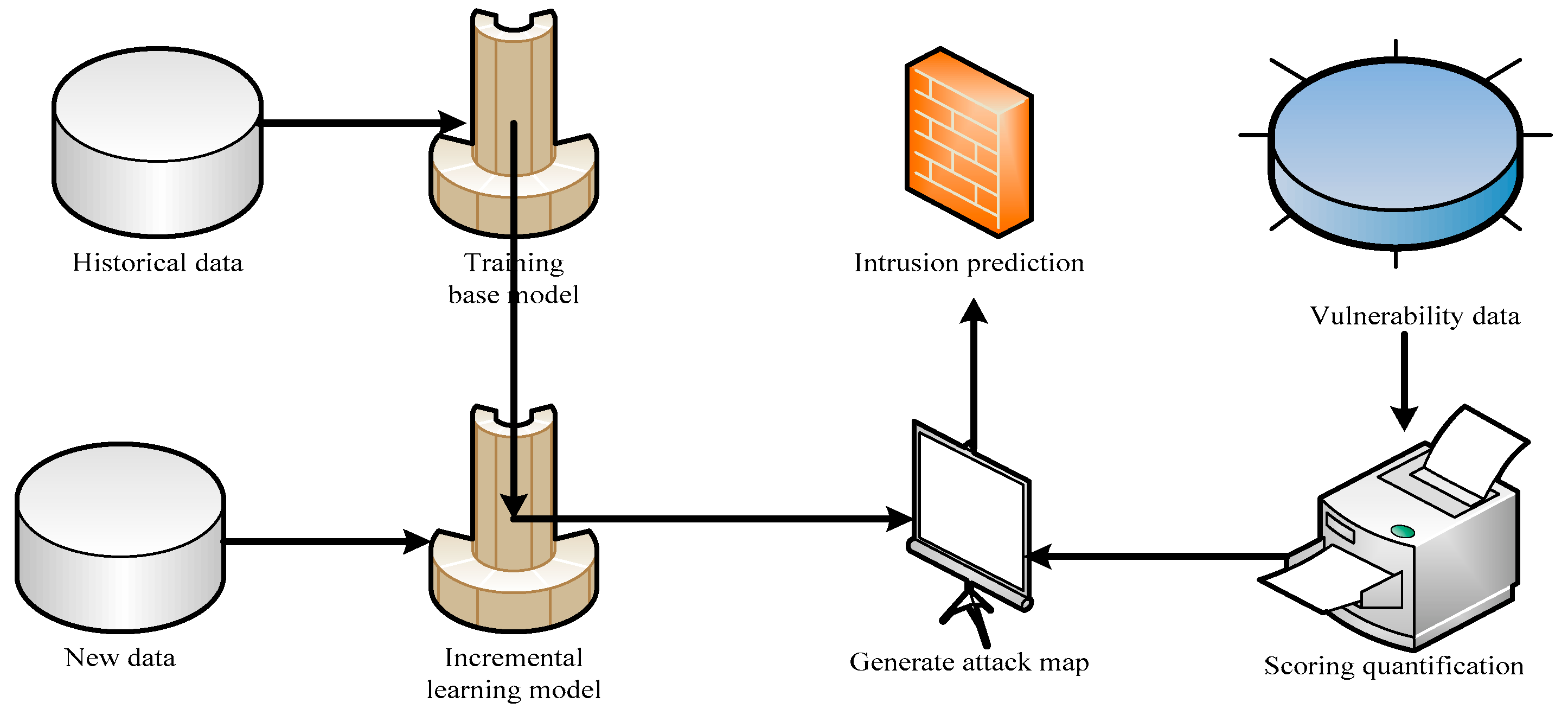
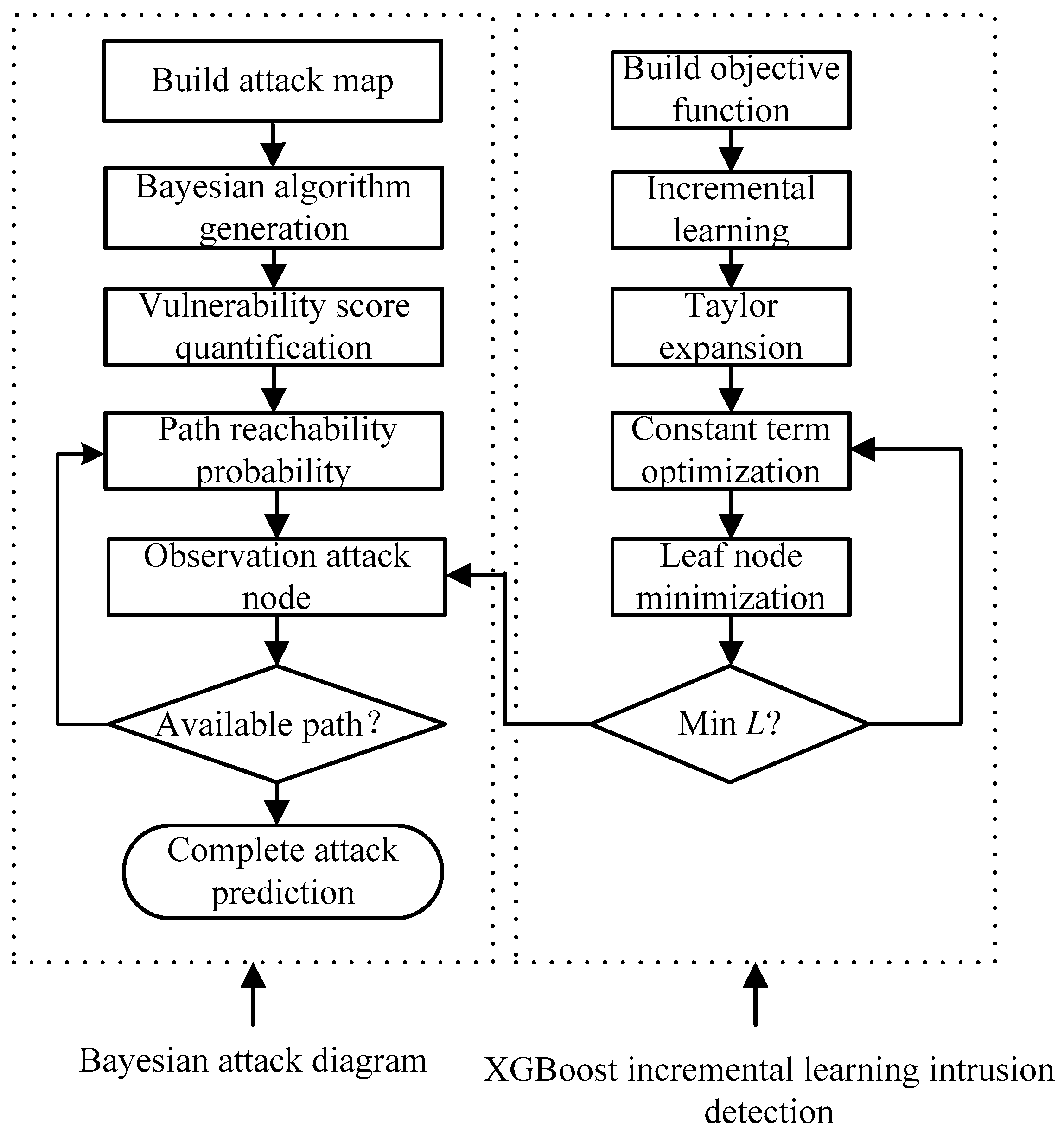
3. A Network Intrusion Detection Method Incorporating a Bayesian Attack Graph and IL

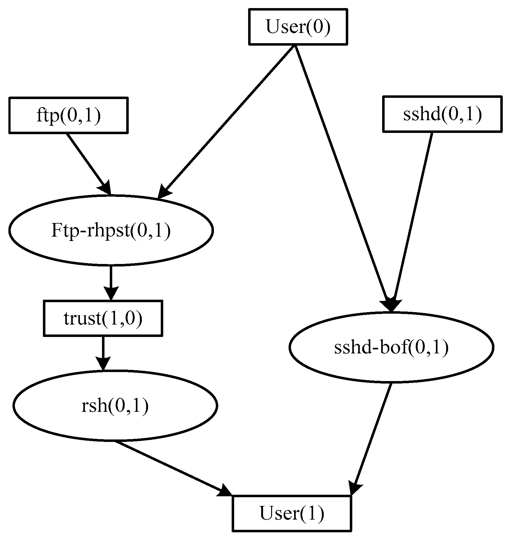
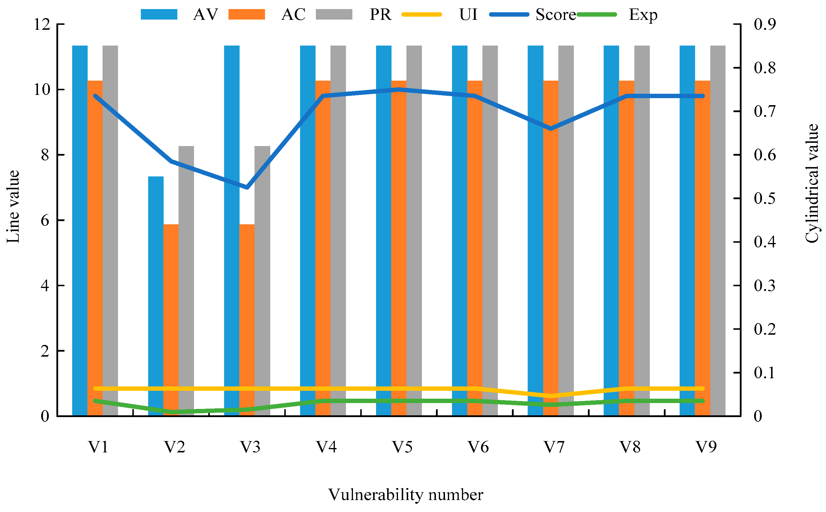
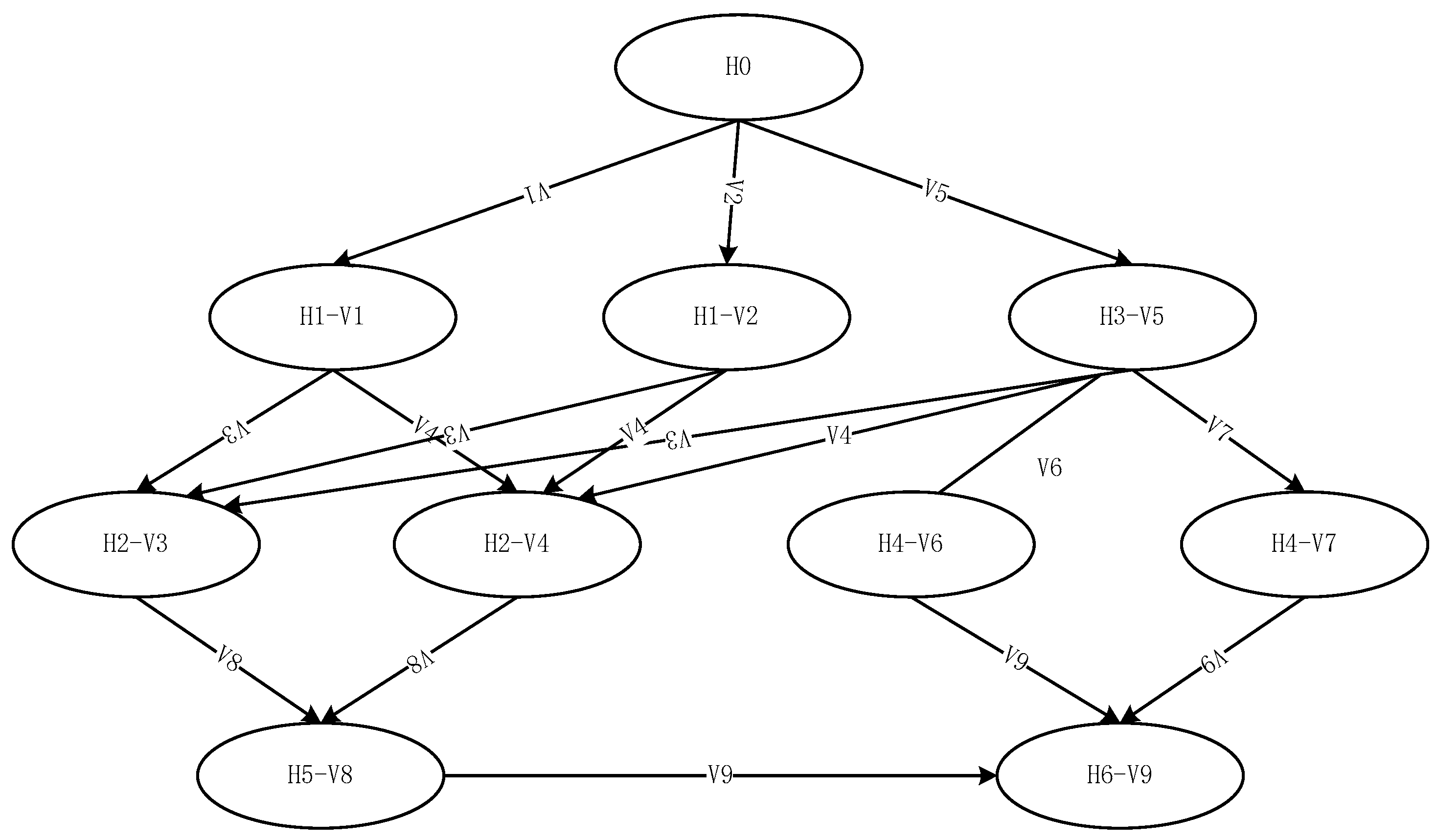
3.1. The Generation of Bayesian Attack Graphs

The computer network system is a complex system composed of a variety of hardware, software, protocols, interfaces, and other components. The software, the hardware system designed for it, and the communication protocols become complex, which resultsin more and more security vulnerabilities. Therefore, attackers often use computer vulnerabilities to carry out attacks. Compared with the past, attacks are not single-step attacks, but multi-step, multi-stage, and multi-target complex attacks. Attackers use the correlation between vulnerabilities to improve their permissions in the system until theyreach their attack goal. The attack graph to be built in this study is the path probability prediction for this vulnerability attack. An attack graph is a kind of directed graph that can show the node’s security and the attacker’s attack path. The state attack diagram contains all possible states of the network system that can be attacked and the transfer relationship among all possible states. The state attack diagram obviously lacks specific state transfer conditions and clear attack paths, which arevery unintuitive. Moreover, with the expansion of the network scale, the global state of the network exponentially expands, and the state attack graph then risks state explosion and is difficult to apply to large-scale networks [18]. The attribute attack graph generally has two types of nodes and edges. The two types of nodes are the conditional node and the vulnerability node. The former indicates the current authority obtained by the attacker and the latter indicates the authority that the attacker can obtain after exploiting the vulnerability of the node. The two types of edges are the edges pointed from the conditional node to the vulnerability node and the edges pointed from the vulnerability node to the conditional node. The former indicates the preconditions required to attack the vulnerability node, and the latter indicates the privileges that can be obtained after attacking the vulnerability. The attribute attack graph is shown in Figure 1.

The rectangular nodes in Figure 1 represent the conditional nodes and the elliptical nodes represent the vulnerability nodes. User (0) and User (1) indicate that the attacker has user access to host 0 and host 1; ftp (0,1) indicates that host 0 can access the ftpd service of host 1; trust (0,1) indicates that host 0 trusts host 1; and Sshd (0,1) indicates that host 0 can access the sshd service of host 1. Bayesian attack graph technology relies on the Bayesian network to show the association relationship between the host nodes of the network system where the attack occurs and is established, and its core lies in the modeling representation, generation, and quantification of the attack graph. To portray the association relationship between vulnerabilities and discover the attacker’s attack intention, a Bayesian attack graph model is proposed in this chapter [19]. The model contains vulnerability exploitation nodes and their weights, directed edges and their weights, relationships of nodes, static reachability probabilities of nodes, and dynamic reachability probabilities of nodes. The above network elements are defined sequentially as $S,E,R,P,P_a,P_b,P_c$. $S=\{S_{begin}\cup S_{other}\}$ is the set of attribute nodes of the network, where $S_{begin}$ denotes the set of starting nodes of the attack graph and $S_{other}$ is the set of nodes other than the starting nodes. $E$ denotes the set of directed edges in the Bayesian attack graph, and $E_{S1:S2}:S1\to S2$ denotes the precondition that the authority of the current attacker at the $S1$ node satisfies the motivating node $S2$. $R=<S_i,R_i>$ denotes the relationship between the antecedent node and the successor node. $R_i\in \{AND,OR\}$ indicates the AND and OR relationships between the antecedent node and the successor node. The AND relationship indicates that the node can be attacked only if all the preconditions of the node are satisfied, while the OR relationship indicates that the node can be attacked as long as any one of the preconditions is satisfied.

In the attack graph, $P$ is the weight on the directed edge that represents the probability of launching an attack on a successor node if the predecessor node has been compromised. $P_a$ denotes the probability of successful exploitation of the node vulnerability in the Bayesian attack graph and thus gaining privileges. $P_b$ denotes the static reachability probability of the node in the representation of the Bayesian attack graph. Its calculation is expressed as Equation (1).

$$P_b(S_i)=\left\{\begin{array}{l}{P}_a(S_i)\cdot {\displaystyle \prod _{j=1}^n{P}_b(S_i)\cdot P(S_i\left|S_j\right.),S_{i}AND{S}_j}\\ P_a(S_i)\cdot [1-{\displaystyle \prod _{j=1}^n(1-P_b(S_i))\cdot P(S_i\left|S_j\right.)}],S_{i}OR{S}_j\end{array}\right.,$$

(1)

In Equation (1), $S_j$ is the parent node. $S_i$ is the child node. $n$ is the number of node setsand $P(S_i\left|S_j\right.)$ represents the probability of attacking a child node among the parent nodes. The first row represents the static reachability probability when the node is an AND relationship, and the second row represents the static reachability probability when the node is an OR relationship. The dynamic reachability probability of the node $P_b$$S_i$ indicates that the reachability probability of its predecessor $S_j$ and successor $S_k$ changes when the node is attacked. Firstly, the dynamic reachability probability of the node $S_i$ is set to one. The calculation for the dynamic reachability probability of the predecessor node is expressed as Equation (2).

$$P_c(S_j\left|S_i\right.)=\frac{P(S_i\left|S_j\right.)\cdot P_b(S_j)}{P_b(S_i)},$$

(2)

In addition, the dynamic reachability probability of $S_k$ is expressed as Equation (3) depending on the relationship between the node $S_i$ and the successor node $S_k$ [20].

$$P_c(S_k\left|S_i\right.)=\left\{\begin{array}{l}{P}_a(S_k)\cdot {\displaystyle \prod _{j=1}^n{P}_b(S_j)}\cdot P(S_k\left|S_j\right.),S_{i}AND{S}_k\\ P_a(S_k)\cdot [1-{\displaystyle \prod _{j=1}^n(1-P_c(S_i)\cdot P(S_k\left|S_j\right.))}],S_{i}OR{S}_k\end{array}\right.,$$

(3)

In Equation (3), the first row represents the dynamic reachability probability when the nodes are AND relations, and the second row represents the dynamic reachability probability when the nodes are OR relations. Meanwhile, this study relies on CVSS3.0 for the calculation of the vulnerability exploitation success rate of the nodes in the Bayesian attack graph. The score of the base dimension of the vulnerability mainly measures the danger of the inherent characteristics of a vulnerability. It is determined by the exploitability indicator of the vulnerability, the impact generated by exploiting the vulnerability, and the impact range of exploiting the vulnerability. Therefore, the calculation for the score of the base dimension of a vulnerability can be expressed as Equation (4).

$$Score=\left\{\begin{array}{l}MIN(\alpha (EXP+imp),10),Scope=changed\\ MIN(EXP+imp,10),Scope=unchanged\end{array}\right.,$$

(4)

In Equation (4), $EXP$ represents the exploitability indicator of the vulnerability, and $imp$ is the impact indicator of the vulnerability. $Scope=changed$ indicates that if the attacker exploits the vulnerability and requires the participation of other users, then $\alpha$ is the scope change weight. $Scope=unchanged$ indicates that the exploited vulnerability only affects the resources in the same environment. Combining the static and dynamic reachability probability in the Bayesian attack graph, the reachability probability of all nodes in the network path can be multiplied cumulatively, and the formula is shown in (5).

$$P(Path)={\displaystyle \prod P_b(S_i)ORP(Path)}={\displaystyle \prod P_c(S_i)\in Path},$$

(5)

By giving the initial node of the attack or the attacked node, it is necessary to find all possible attack paths of the attacker and calculate the reachable probability of each path to find out the most likely attack path to be taken to discover the next attack target of the attacker. Therefore, Bayesian attack graphs can predict the set of potential attack paths for network attacks.

3.2. IL Intrusion Detection Method Based on XGBoost

Although Bayesian attack graphs have been able to perform complete attack prediction, the attack characteristics for intrusions still rely on the professional experience of network security experts and the historical data of the attacked [21]. Therefore, pure Bayesian attack graphs are weak for detecting unknown security events, and it is necessary to combine attack graph techniques with intrusion detection techniques to adapt to the network. When an intrusion detection system detects an attack in the network, the system can perform an active update of the attack graph. Therefore, the study proposes an IL-based intrusion detection method that enables the model to learn the features of new data quickly and ensures the predictive capability of the model for new data. The method is then combined with a Bayesian attack graph to achieve real-time prediction of attacker attacks. The network attack methods targeted by this model mainly include seven types: brute force, Heartbleed, Botnet, Denial of Service (DoS), Distributed Denial of Service (DDoS), Web attacks, and Infiltration of the network from inside. The framework for combining Bayesian attack graphs and IL intrusion detection methods is shown in Figure 2.

As shown in Figure 2, when using the IL approach for intrusion detection with new data to continue training the base model, the amount of new training data is not large and again allows the model to learn the feature distribution of the new data, improving the prediction accuracy of the model. In the intrusion detection method based on IL built in this study, firstly, a Bayesian attack graph is generated through the scoring and correlation of the vulnerability database, and the attack graph is quantified. After the IL is trained with history and new data, the quantitative attack is expressed as the node reachability probability to observe the attack behavior. Finally, the prediction network is analyzed in the section on dynamic reachability probability.

In this study, XGBoost is used as the base model. Firstly, assuming that the loss function of the dataset $T=\{(x_1,y_1),(x_2,y_2),\dots ,(x_n,y_n)\}$ is ${\displaystyle \sum _{i}l(y_i,{\widehat{y}}_i)}$ and the regularization term is $\mathrm{\Omega }(f)$. The overall objective function is expressed as Equation (6).

$$L(\mathrm{\Theta })={\displaystyle \sum _{i}l(y_i,{\widehat{y}}_i)}+{\displaystyle \sum _k\mathrm{\Omega }(f_k)}k,$$

(6)

In Equation (6), $i$ denotes the ith sample. $k$ denotes the krd tree. ${\widehat{y}}_i$ is the predicted value of the ith sample. Formula (6) serves as the base model for XGBoost incremental learning, and its application conditions lie in the training process of intrusion detection methods. In the training, the new data and the old data will train the intrusion detection model together, and after the feature extraction of the new data, the introduction Formula (6) can be used to build a new incremental learning model. Since XGBoost uses the gradient boosting method, the new tree is fitted with the residuals of the previous tree. The predicted value of the ith sample of the tth tree is represented by $x_i$. Then, the predicted value of the model is expressed as Equation (7).

$${\widehat{y}}_i={\displaystyle \sum _{k=1}^t{f}_k(x_i)=}{\widehat{y}}_i^{t-1}+f_t(x_i),$$

(7)

Therefore, the objective function is rewritten as Equation (8).

$$L^{(t)}={\displaystyle \sum _{i=1}^{n}l(y_i,y_i^{t-1}+f_t(x_i))+{\displaystyle \sum _k\mathrm{\Omega }(f_k)}},$$

(8)

Therefore, the task at hand is to find the point $f_t(x_i)$ that minimizes the value of the objective function, and XGBoost obtains an approximation by performing a second-order Taylor expansion of the objective function at the point $f_t(x_i)=0$, i.e.,

$$L^{(t)}\cong {\displaystyle \sum _{i=1}^n[l(y_i,y_i^{(t-1)})+g_i{f}_t(x_i)+\frac{1}{2}{h}_i{f}_t^2(x_i)]+{\displaystyle \sum _k\mathrm{\Omega }(f_k)}},$$

(9)

In Equation (9), $g_i=l^{\prime }(y_i,{\widehat{y}}_i^{(t-1)})$, $h_i=l^{″}(y_i,{\widehat{y}}_i^{(t-1)})$, while the regularization is calculated by $\mathrm{\Omega }(f)=\gamma T+\frac{1}{2}\lambda {‖\omega ‖}^2$. It is known that $l(y_i,{\widehat{y}}_i^{(t-1)})$ is a constant term, so the problem of solving the minimum of the objective function is not related to it. At the same time, since the structure of the previous $t-1$ tree has been determined, the regularization term of the previous $t-1$ tree is a constant, so here the regularization term can be split into a variable and a constant term in the following way. The constant term, which is related to solving the minimum of the objective function, can be deleted. So the objective function expression can be optimized as Equation (10).

$$L^{(t)}={\displaystyle \sum _{i=1}^n[g_i{f}_i(x_i)+\frac{1}{2}{h}_i{f}_t^2(x_i)]+\mathrm{\Omega }(f_t)},$$

(10)

All samples are grouped by leaf nodes.

$$L^{(t)}={\displaystyle \sum _{j=1}^T[({\displaystyle \sum _{i\in I_j}{g}_i})w_j+\frac{1}{2}({\displaystyle \sum _{i\in I_j}{h}_i+\lambda })w_j^2]+\gamma T},$$

(11)

In Equation (11), $I_j$ denotes the set of training samples under the jth leaf node. $G_j={\displaystyle \sum _{i\in I_j}{g}_i}$, $H_j={\displaystyle \sum _{i\in I_j}{h}_i}$, where $G_j$ denotes the cumulative sum of the first-order partial derivatives of all samples in the leaf node $j$, and $H_j$ denotes the cumulative sum of the second-order partial derivatives of all samples in the leaf node $j$. Both of theseare constants, so the expression of the objective function is optimized as Equation (12).

$$L^{(t)}={\displaystyle \sum _{j=1}^T[G_j{w}_j+\frac{1}{2}(H_j+\lambda )w_j^2]}+\gamma T,$$

(12)

At this point, the only variable left in the expression is the weight vector of the tth tree $w$, and finding the min of the objective function is transformed into finding the cumulative sum. In addition, for the leaf node $j$, its objective function expression is a quadratic equation, as shown in Equation (13).

$$f(w_j)=G_j{w}_j+\frac{1}{2}(H_j+\lambda )w_j^2,$$

(13)

Therefore, the minvalue point of the leaf node $j$ is expressed as ${w^{\prime }}_j=-G_j/H_j+\lambda$. When the objective functions of the leaf nodes are taken to the min value, the objective function is taken to the min value expressed as Equation (14).

$$L_{\min }^{(t)}=-\frac{1}{2}{\displaystyle \sum _{j=1}^T\frac{G_j^2}{H_j+\lambda }+\gamma T},$$

(14)

In practical application scenarios, intrusion detection data are constantly being added and the distribution of data is likely to be changing constantly. The most direct way of IL is to train a model with new intrusion detection data and a base model with historical intrusion detection data to identify the base features of the intrusion detection data. Then, it needs to learn the latest data features with recently collected intrusion detection data. XGBoost model is an additive model, which trains $t$ trees from historical data, then the classification result of the model on samples is $t$ trees A weighted fusion of the classification results. When the new historical data are collected, the new intrusion detection data are used to train $m$ trees to learn the features of the new data based on the original $t$ trees. When the training is completed, the classification result of the model on the samples is the weighted fusion of the classification results of $t$ trees of the base model and $m$ trees of the new model, as shown in Equation (15).

$${\widehat{y}}_i={\displaystyle \sum _{k=1}^{t+m}{f}_k(x_i)={\widehat{y}}_i^{(t+m-1)}+f_{(t+m)}(x_i)},$$

(15)

Such classification results consider both data features of historical data and new data, and only new intrusion detection data are used to train the model greatly saving computational resources and reducing training time. The final flow of the intrusion prediction method incorporating the Bayesian attack graph and XGBoost IL is shown in Figure 3.

In Figure 3, this study proposes an IL-based intrusion detection method that enables the model to learn the features of new data quickly and ensures the predictive capability of the model for new data. The method is then combined with a Bayesian attack graph to achieve real-time prediction of attacker attacks.

4. Performance Analysis of Network Intrusion Detection Methods Incorporating Bayesian Attack Graph and IL

4.1. Path Prediction Experiments with Bayesian Attack Graphs

To verify the performance of the proposed Bayesian attack graph-based network attack prediction method in this paper, the study built a network system through a mail server, Apache server, DNS server, personal PC, MySQL server, and FTP server. In addition, an IL-based intrusion detection system was installed on each host to identify attacker attack behavior. Among them, the vulnerability information on each host is shown in

Table 1. Distribution of Cited References.

Literature Field	Literature Number	Sketch
Introduction to Network Attack	[1,2,3]	Network intrusion security literature introduced in the background
Wireless sensor networks	[4,5]	Modern English for Wireless Sensor Networks Introduced as a Background
DL	[6,7]	Application of DL in Network Technology
Network Intrusion Attack Graph Technology	[7,8,9,10,11,20]	Optimization results of attack graph technology by domestic and foreign scholars
Other network security information technology	[12,13,14,15,16,17]	Domestic and foreign scholars’ detection methods for network intrusion
Internet of Things and Computer Communication	[17,18,19,21]	Research on new application of network security technology and information transmission

. For the node vulnerability utilization success rate, this paper used CVSS3.0 general vulnerability scoring system to quantify it here. CVSS3.0 was released by the National Vulnerability Database (NVD) of the United States and kept the vulnerability data updated. CVSS3.0 comprehensively measured the harmfulness of vulnerabilities from three dimensions: the basic dimension of vulnerabilities, the time dimension, and the environment dimension. CVSS3.0 combined these three dimensions to give a specific score for vulnerabilities. The range of the score was [0, 10], where the vulnerability with a score between 0 and 3.9 was a low-risk vulnerability; the vulnerability with a score of 4 to 6.9 was a medium-risk vulnerability; the vulnerability with a score of 7 to 8.9 was a high-risk vulnerability; and the vulnerability with a score of 9 to 10 was a super-risk vulnerability. The Bayesian attack graph is an attack graph model that combines the Bayesiannetwork and attack graph technology. It uses Bayesian networks to represent the correlation between attack behaviors among host nodes in a network system, thereby establishing an attack graph structure. Its core lies in the modeling, generation, and quantification of attack graphs. Research on uncertainty handling during both qualitative and quantitative risk assessment procedures is a growing field. Theoretical contributions, explanatory uncertainty, cognitive uncertainty, and integration of cognitive and interpretative uncertainty processing in scientific and technological literature [22]. At the same time, this experiment needs to quantify the node and edge weight of the Bayesian attack graph, where the node weight represents the current node vulnerability utilization success rate. In addition, the hosts and vulnerabilities are numbered here for the convenience of subsequent presentations.

In

Table 2. Host and Vulnerability Information of Network Framework.

Host Name	Function Description	Host Number	Vulnerability Name	Vulnerability Number
Apache server	Provide Web Server services	H1	CVE-2020-13942	V1
			CVE-2020-15778	V2
Mail server	Be responsible for email sending and receiving management	H2	CVE-2018-19518	V3
			CVE-2018-6789	V4
DNS server	Domain name resolves to IP address	H3	CVE-2020-1350	V5
PC	Personal office machine	H4	CVE-2019-0708	V6
			CVE-2021-1675	V7
FTP server	Provide file storage and access services	H5	CVE-2019-12815	V8
MySQL server	Provide database services	H6	CVE-2016-6662	V9

, the vulnerabilities in V1–V9 are, in order, malicious requests to execute arbitrary code through the server, vulnerabilities that can execute illegal commands, attacks against authentication, code executed in an application context, code that bypasses authentication to execute code with local SYSTEM account privileges, remote code execution vulnerability in Remote Desktop Services, seizing control on a domain controller with SYSTEM privileges code, code that bypasses permission to copy FTP server files, and code that injects malicious environment configuration into My SQL configuration files. The scores of the above nine vulnerabilities are represented by the vulnerability CVSS scores shown in Figure 4.

In Figure 4, AV denotes the attack path score of the vulnerability. AC denotes the attack complexity score of the vulnerability. PR denotes the required privilege score of the vulnerability, and UI denotes the user interaction score of the vulnerability. Exp denotes the exploitable index of the vulnerability, and Score is the composite score calculated by Equation (4) in this paper. Figure 4 shows that V1, V4, V5, V6, V8, and V9 are ultra-dangerous vulnerabilities, and the rest are high-order vulnerabilities. As shown in Figure 4, the vulnerability with the highest comprehensive score was V5. As shown in Figure 4, V1, V4, V5, V6, V8, and V9 were ultra-dangerous vulnerabilities, and the rest were high-order vulnerabilities. Based on the above network system environment and vulnerability information, this study used the Bayesian algorithm to construct the unweighted Bayesian attack graph, as shown in Figure 5.

From Figure 5, nodes H6-V9 are the endpoints of the entire attack graph. The algorithm found all the attack paths from the attacker’s initial node H0 to the endpoints of the attack graph H6-V9 and calculated the reachability probability of each path. The reachability probability of each node and each path in the graph are shown in

Table 3. Bayesian Attack Graph Node Reachability Probability and Path Reachability Probability.

Node	Node Reachability Probability	Path Number	Route	Path Reachability Probability
H1-V1	0.46	Path-A	H0→H1-V1→H2-V3→H5-V8→H6-V9	0.0036
H1-V2	0.1	Path-B	H0→H1-V1→H2-V4→H5-V8→H6-V9	0.0116
H2-V3	0.13	Path-C	H0→H1-V2→H2-V3→H5-V8→H6-V9	0.0008
H2-V4	0.41	Path-D	H0→H1-V2→H2-V4→H5-V8→H6-V9	0.0032
H3-V5	0.47	Path-E	H0→H3-V5→H2-V3→H5-V8→H6-V9	0.0037
H4-V6	0.22	Path-F	H0→H3-V5→H2-V4→H5-V8→H6-V9	0.0116
H4-V7	0.14	Path-G	H0→H3-V5→H4-V6→H6-V9	0.0259
H5-V8	0.24	Path-H	H0→H3-V5→H4-V7→H6-V9	0.0165
H6-V9	0.25	/	/	/

.

From Table 3, the reachability probability of nodes H1-V1, nodes H3-V5, and nodes H2-V4 were higher, so they were more likely to be compromised by attackers. In addition, Path-G had the highest path reachability probability, and the attacker was most likely to execute the attack according to Path-G, which contained the high-risk nodes H3-V5. Combining the node and path reachability probability, the node that the attacker was most likely to attack was H3-V5.

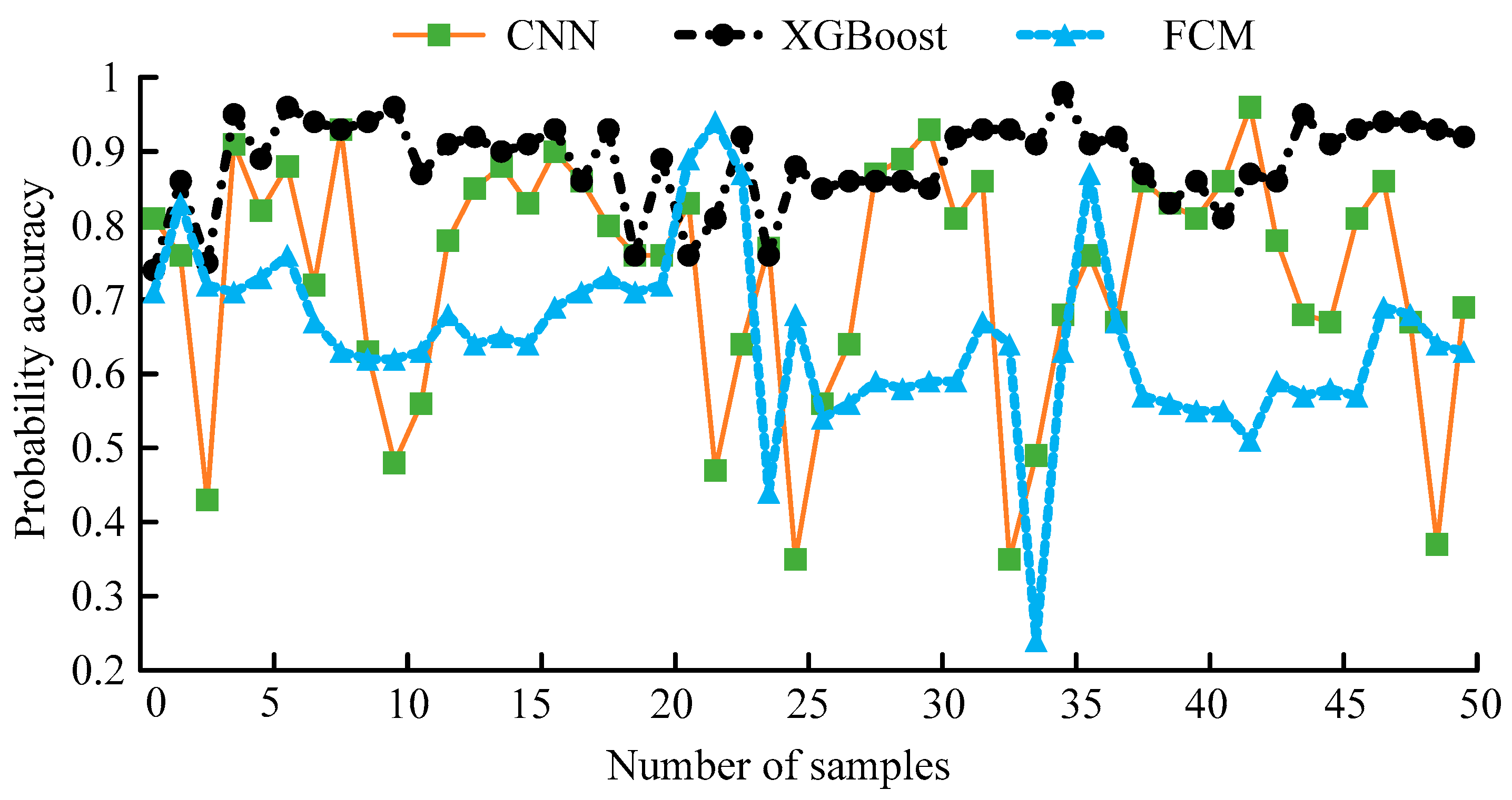
4.2. IL for Intrusion Detection Performance Verification Analysis

To verify that the XGBoost IL algorithm utilized in this study can be effectively applied to network sensor intrusion detection with Bayesian attack graphs, this study was tested by training and simulation with the CSE-CIC-IDS-2018 dataset created jointly by the G Canadian Institute for Cyber Security Research. This dataset contained much information on the network flow duration, the total number of forward-backward packets, and the total number of forward packets. At the same time, the dataset incorporated more advanced and recent attacks. With the change innetwork behavior and mode and the development of intrusion, it is very necessary to change from static and one-time datasets to more dynamic datasets. These datasets not only reflect the traffic combination and intrusion at that time but are also modifiable, scalable, and reproducible. To overcome these shortcomings, the dataset designed a systematic method to generate the dataset to analyze, test, and evaluate the intrusion detection system, focusing on the network-based anomaly detector. The main goal of this project is to develop a systematic method to generate a diversified and comprehensive benchmark dataset for intrusion detection based on the creation of user profiles that contain the abstract representation of events and behaviors seen on the network. These profiles will be combined to generate a different set of datasets. Each dataset has a unique set of characteristics that cover a part of the evaluation domain.

In this experiment, since the XGBoost model is a tree model, there is no need to normalize the data. In addition, the XGBoost model itself can handle missing values, so there is no need to fill or remove missing values. For the outliers, statistical analysis was performed and found to be too small, so they were deleted here. For recurring data records, only their first occurrence was retained, and the rest of the redundant data records were deleted. After preprocessing, the information of the sample dataset is shown in

Table 4. Effective Sample Quantity Information After Data Preprocessing.

Date	Number of Samples	Date	Number of Samples
14 February 2018	392,909	22 February 2018	443,070
15 February 2018	426,094	23 February 2018	445,761
16 February 2018	470,336	28 February 2018	470,336
20 February 2018	3,447,677	1 March 2018	128,073
21 February 2018	522,559	2 March 2018	517,200

.

To conduct experiments on IL, the data from 14 February 2018 to 23 February 2018 in the dataset were used here as the training set for the base model, and the data from 28 February 2018 were used as the incoming training set data to continue training the incremental model on the base model. For comparison with incremental training, the data from 14 February 2018 to 23 February 2018 were used as the training set for full training, and the data from 1 March 2018 and 2 March 2018 were used as the test set data for these three training methods. In this experiment, the conventional confusion matrix values were chosen as the experimental evaluation metrics to evaluate the performance of the IL-based intrusion detection method. The specific results are listed in

Table 5. Evaluation Indicators of Three Models.

/	Acc	Prec	Re	f1-Score	AUC
Base model	0.734	0.602	0.001	0.002	0.500
IL	0.951	0.999	0.815	0.898	0.907
Full training	0.949	0.999	0.807	0.893	0.904

.

In Table 5, the accuracy rate, precision rate, and recall rate were used in this study to evaluate the prediction performance of the model, where AUC represented the area under the ROC and the area surrounding the coordinate axis. In Table 5, the performance of the base model in the test set was very poor, with an accuracy of 0.734 and an accuracy of 0.602 lower than the IL model and the full learning model. In the test set, the proposed IL model had a high accuracy of 0.951, a precision of 0.999, a recall of 0.815, an f1 value of 0.898, and an AUC value of 0.907. These evaluation metrics were not only much higher than the base model, but they were also slightly higher than the full learning model. The main reason for the low recallof the base model in the confusion matrix data was the lower predictive power of the base model for malicious traffic, which was due to the change in the data distribution of malicious traffic in the test set. The training dataset of the base model contained only a small amount of this type of data, so the amount of malicious traffic data of this type was poorly learned, which resulted in little ability to discernnew malicious traffic data in the base model. The f1 and AUC values of the base model indicated that the base model was very poor in the test set. The predictive power of the IL model was slightly higher than that of the full training due to the fact that the distribution of data features in the IL training set was closer to the distribution of data features in the test set. Finally, this study compared different intrusion detection algorithms with the same environment and test data. Fifty samples were randomly selected from the test dataset to compare the intrusion detection performance of Convolutional Neural Networks (CNN), the Fuzzy C-Means (FCM) algorithm, and the XGBoost IL algorithm used in the study, and the specific experimental results are listed in Figure 6.

In Figure 6, among the 50 random samples, the most stable accuracy performance was the XGBoost IL algorithm proposed in the study, followed by the CNN algorithm. In the same data samples, the highest accuracy of CNN network intrusion detection was 0.961, the lowest accuracy was 0.349, and the average accuracy was 0.764. Meanwhile, the highest precision was 0.959, the lowest precision was 0.261, and the average precision was 0.655.

5. Conclusions

To adapt the intrusion detection mechanism to the dynamic changes in the network system, this paper provided an in-depth study of Bayesian attack graph techniques and intrusion detection techniques. The experimental results on the network system vulnerability dataset showed that the IL model had an accuracy of 0.951, a precision of 0.999, a recall of 0.815, an F1 value of 0.898, and an AUC value of 0.907. The performance was much higher than the base model and slightly higher than the full-volume learning model. Meanwhile, among the accuracy performance comparison of different algorithms, the average accuracy of the XGBoost IL algorithm was 0.954, which was higher than that of the CNN network and fuzzy C-mean algorithm. Meanwhile, in the practical application of the attack graph, the model could clearly show the correlation between vulnerabilities, the risk faced by each node, and the next attack movement of the attacker when the node was compromised. The model could update the dynamic reachability probability of each node in real time based on the detection information of the intrusion detection system. The shortcoming of the study is that it is quantified by CVSS scores and the exploitability of its vulnerabilities. However, for the actual network environment, more specific factors should be considered, such as the attacker’s attack frequency.

References

1. Mishra, P.; Varadharajan, V.; Tupakula, U.S.; Pilli, E. A detailed investigation and analysis of using machine learning techniques for intrusion detection. IEEE Commun. Surv. Tutor. 2018, 21, 686–728. [Google Scholar] [CrossRef]
2. Shone, N.; Ngoc, T.N.; Phai, V.D.; Shi, Q. A deep learning approach to network intrusion detection. IEEE Trans. Emerg. Top. Comput. Intell. 2018, 2, 41–50. [Google Scholar] [CrossRef] [Green Version]
3. Gao, X.; Shan, C.; Hu, C.; Niu, Z.; Liu, Z. An adaptive ensemble machine learning model for intrusion detection. IEEE Access 2019, 7, 82512–82521. [Google Scholar] [CrossRef]
4. Ramos, M.D.; Foster, A.D.; Felici, S.; Fos, V.G.; Solano, J.J.P. Gatherer: An environmental monitoring application based on IPv6 using wireless sensor networks. Int. J. Ad Hoc Ubiquitous Comput. 2013, 13, 209–217. [Google Scholar] [CrossRef]
5. Segura-Garcia, J.; Calero, J.M.A.; Pastor-Aparicio, A.; Marco-Alaez, R.; Felici-Castell, S.; Wang, Q. 5G IoT system for real-time psycho-acoustic soundscape monitoring in smart cities with dynamic computational offloading to the edge. IEEE Internet Things J. 2021, 8, 12467–12475. [Google Scholar] [CrossRef]
6. Kim, M. ML/CGAN: Network attack analysis using CGAN as meta-learning. IEEE Commun. Lett. 2020, 25, 499–502. [Google Scholar] [CrossRef]
7. Públio, M.L.; Marcos Vinícius, S.A.; Lilian, K.C.; Marcos, V.M. Security against communication network attacks of cyber-physical systems. J. Control Autom. Electr. Syst. 2019, 30, 125–135. [Google Scholar]
8. Wu, H.; Gu, Y.; Cheng, G.; Zhou, Y. Effectiveness evaluation method for cyber deception based on dynamic bayesian attack graph. In Proceedings of the 2020 3rd International Conference on Computer Science and Software Engineering, Beijing, China, 22–24 May 2020; pp. 1–9. [Google Scholar]
9. Kaynar, K.; Sivrikaya, F. Distributed attack graph generation. IEEE Trans. Dependable Secur. Comput. 2015, 13, 519–532. [Google Scholar] [CrossRef]
10. Li, H.; Wang, Y.; Cao, Y. Searching forward complete attack graph generation algorithm based on hypergraph partitioning. Procedia Comput. Sci. 2017, 107, 27–38. [Google Scholar] [CrossRef]
11. Al Ghazo, A.T.; Ibrahim, M.; Ren, H. A2G2V: Automatic attack graph generation and visualization and its applications to computer and SCADA networks. IEEE Trans. Syst. Man Cybern. Syst. 2019, 50, 3488–3498. [Google Scholar] [CrossRef]
12. Garcia-Pineda, M.; Segura-Garcia, J.; Felici-Castell, S. A holistic modeling for QoE estimation in live video streaming applications over LTE Advanced technologies with Full and Non Reference approaches. Comput. Commun. 2018, 117, 13–23. [Google Scholar] [CrossRef]
13. Chapaneri, R.; Shah, S. Multi-level Gaussian mixture modeling for detection of malicious network traffic. J. Supercomput. 2021, 77, 4618–4638. [Google Scholar] [CrossRef]
14. Wang, H.; Gu, J.; Wang, S. An effective intrusion detection framework based on SVM with feature augmentation. Knowl. Based Syst. 2017, 136, 130–139. [Google Scholar] [CrossRef]
15. Gu, J.; Lu, S. An effective intrusion detection approach using SVM with naïve Bayes feature embedding. Comput. Secur. 2021, 103, 102158. [Google Scholar] [CrossRef]
16. Hakim, L.; Fatma, R. Influence analysis of feature selection to network intrusion detection system performance using nsl-kdd dataset. In Proceedings of the 2019 International Conference on Computer Science, Information Technology, and Electrical Engineering (ICOMITEE), Jember, Indonesia, 16–17 October 2019; pp. 217–220. [Google Scholar]
17. Laghrissi, F.E.; Douzi, S.; Douzi, K.; Hssina, B. Intrusion detection systems using long short-term memory (LSTM). J. Big Data 2021, 8, 65. [Google Scholar] [CrossRef]
18. Alsughayyir, B.; Qamar, A.M.; Khan, R. Developing a network attack detection system using deep learning. In Proceedings of the 2019 International Conference on Computer and Information Sciences (ICCIS), Aljouf, Saudi Arabia, 3–4 April 2019; pp. 1–5. [Google Scholar]
19. Belouch, M.; El Hadaj, S.; Idhammad, M. Performance evaluation of intrusion detection based on machine learning using apache spark. Procedia Comput. Sci. 2018, 127, 1–6. [Google Scholar] [CrossRef]
20. Poolsappasit, N.; Dewri, R.; Ray, I. Dynamic Security Risk Management Using Bayesian Attack Graphs. IEEE Trans. Dependable Secur. Comput. 2012, 9, 61–74. [Google Scholar] [CrossRef]
21. Polatidis, N.; Pimenidis, E.; Pavlidis, M.; Papastergiou, S.; Mouratidis, H. From product recommendation to cyber-attack prediction: Generating attack graphs and predicting future attacks. Evol. Syst. 2020, 11, 479–490. [Google Scholar] [CrossRef] [Green Version]
22. Yazdi, M.; Kabir, S.; Walker, M. Uncertainty handling in fault tree based risk assessment: State of the art and future perspectives. Process Saf. Environ. Prot. 2019, 131, 89–104. [Google Scholar] [CrossRef]
Figure 1. Attribute Attack Graph.
Futureinternet 15 00128 g001
Figure 2. A Framework for the Combination of Bayesian Attack Graph and IL Intrusion Detection Method.
Futureinternet 15 00128 g002
Figure 3. Network Intrusion Detection Process Based on Bayesian Attack Graph and IL.
Futureinternet 15 00128 g003
Figure 4. Vulnerability CVSS Score and Availability Information.
Futureinternet 15 00128 g004
Figure 5. Attack Graph With Node Path Not Weighted.
Futureinternet 15 00128 g005
Figure 6. Testing of Different Intrusion Detection Methods in the Dataset.
Futureinternet 15 00128 g006