
Performance of Path Loss Models over Mid-Band and High-Band Channels for 5G Communication Networks: A Review

 , , and
Abstract
1. Introduction
- We compared the applicability of machine learning models against existing current 5G empirical models at the high-band frequency spectrum.
- We evaluated the applicability of these models in the context of coexistence studies in the selected mid-band and high-band spectrums.
- Considerations for potential scenarios involving additional environmental factors were considered when examining the study of frequency band propagation analysis that are candidates for 6G systems.
2. Channel Propagation Characteristics
2.1. Characteristics of Mid-Band and High-Band Frequency Spectra
2.1.1. Short Wavelength
2.1.2. Abundant Bandwidth
2.1.3. Propagation Loss
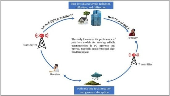
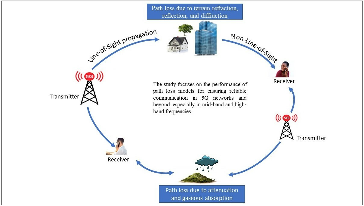
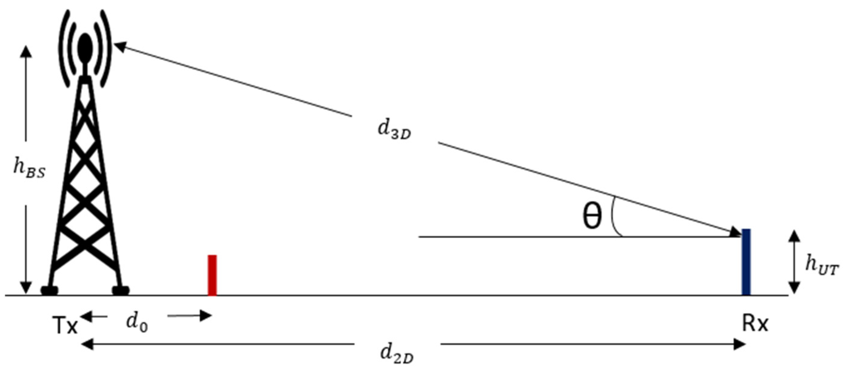
2.2. Path Loss in Wireless Communications
3. Path Loss Models
3.1. Empirical Models
3.1.1. Early Empirical Models
- A.
- Okumura Model
- B.
- Okumura–Hata Model
- C.
- COST-231 Hata Model
3.1.2. Current Empirical Models
- A.
- 3GPP TR 38.901 Model [39]
- i.
- ii.
- B.
- Close-In (CI) Free Space Reference Distance Path Loss Model [23]
- C.
- Alpha–Beta–Gamma (ABG) Model [23]
- D.
- FI Model [46]
3.2. Machine Learning Models
4. Performance Metrics for Path Loss Models
- A.
- Mean Square Error (MSE)
- B.
- Mean Absolute Error (MAE)
- C.
- Mean Error (ME)
- D.
- R2 Score
5. Reviewed Papers on Empirical-Based Path Loss Models
5.1. Performance Evaluation of Empirical Path Loss Models in Urban Environment
5.2. Performance Evaluation of Empirical Path Loss Models in Indoor Environment
6. Reviewed Papers on Machine-Learning-Based Path Loss Models
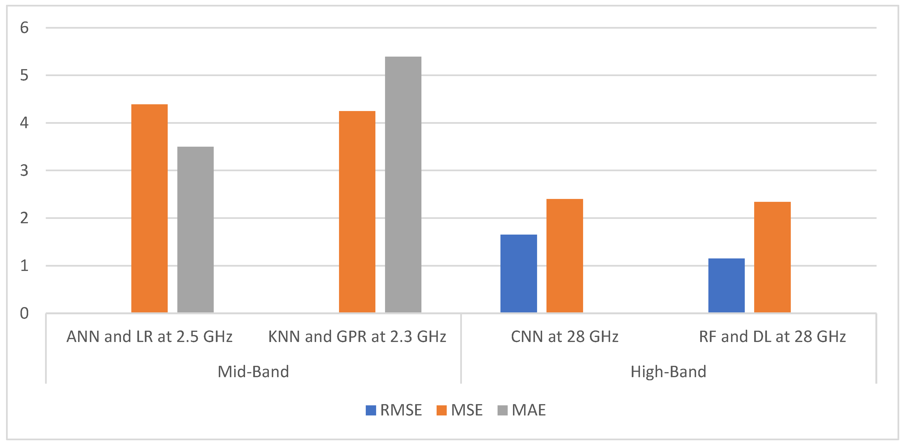
6.1. Assessment of Machine Learning Path Loss Models in Outdoor Urban Environments
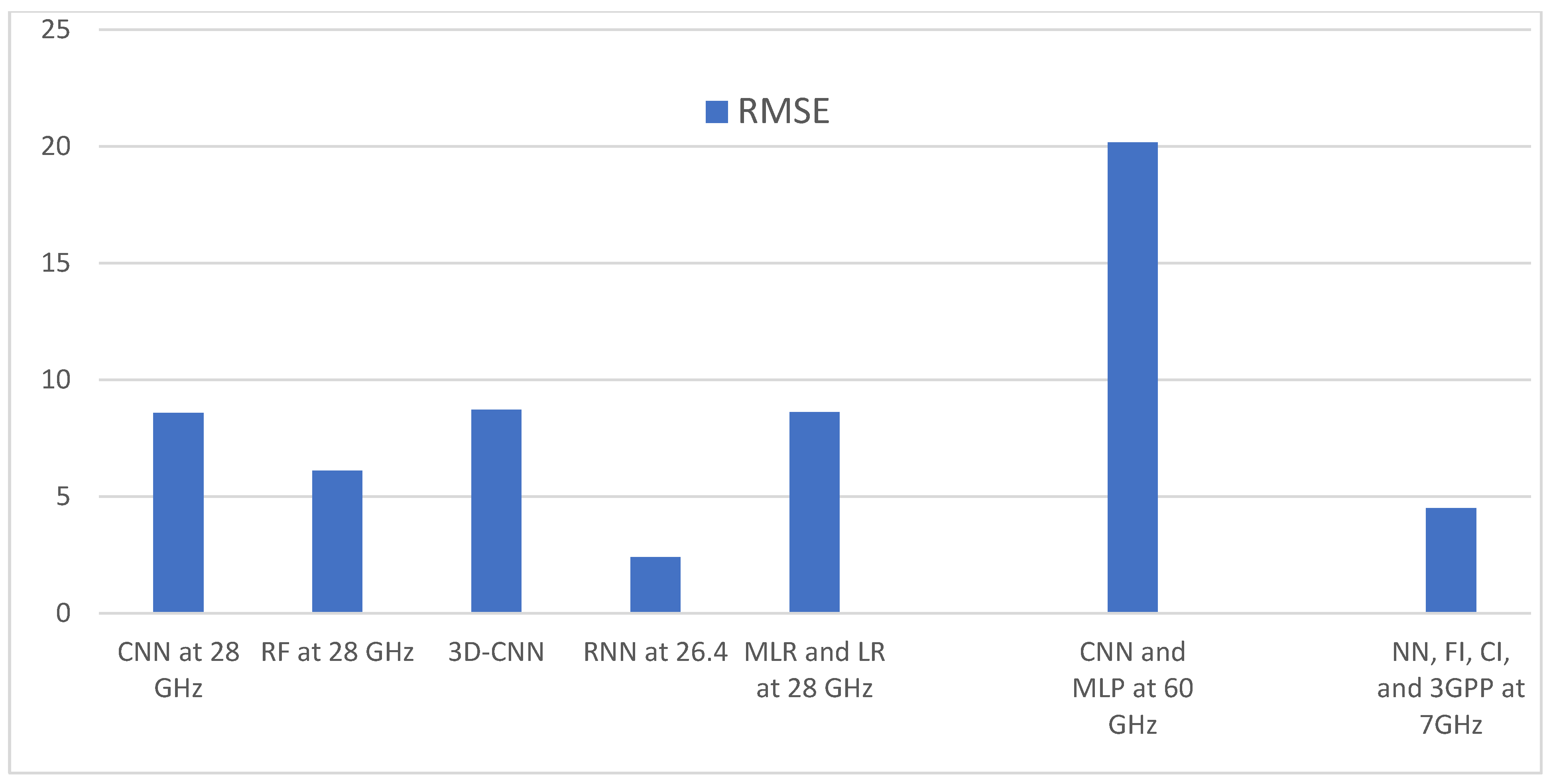
6.2. Evaluation of High-Band Machine Learning Path Loss Models in Urban Environments
6.3. Evaluation of Indoor Machine Learning Path Loss Models
7. Open Research Issues
7.1. Research Gaps
- i.
- Dynamic urban environments: Urban environments are highly dynamic, with changes in building layouts, vegetation, and infrastructure occurring frequently. The current empirical models, such as the ABG, CI, FI, and 3GPP, may not be able to account for these dynamic changes adequately, resulting in inaccuracies in path loss predictions. Integrating real-time or dynamic elements into empirical models is a research gap that needs to be addressed. Hence, they need to be improved to fit the worst-case scenario of the urban environment and to make them reliable in any other urban environment. The current empirical models may not adequately capture or account for these interference and multipath effects, leading to inaccurate predictions.
- ii.
- Inadequate integration of machine learning techniques: Machine learning techniques, such as the random forest model and neural networks, have shown promise in improving path loss prediction accuracy across the considered mid-band and high-band frequency spectrums. However, limited research exists on effectively integrating these techniques into empirical models for path loss in the mid-band frequency spectrum in urban environments. Exploring the potential of machine learning-based approaches and their integration into existing models is an important research gap.
- iii.
- Lack of validation in real-world scenarios: Empirical models developed for predicting path loss in mid-band and high-band frequencies in urban and suburban environments may not have been extensively tested and validated in real-world scenarios. The absence of comprehensive field measurement and validation studies can introduce uncertainties and limit the reliability and accuracy of the models.
- iv.
- Inadequate consideration of complex environment: The empirical models that were used did not sufficiently account for factors such as high-rise buildings, vegetation, and diverse land use patterns, leading to inaccuracies in path loss estimation. Developing models that can accurately capture and incorporate the characteristics of complex urban and suburban environments is a significant research gap.
- v.
- Lack of relevant features on labeled training data: There is a shortage of relevant features on labeled datasets, as in the case of the random forest model that outperformed other chosen models [77,83]. This scarcity of relevant features that greatly impact the prediction poses a significant research gap as it hinders the development and deployment of an accurate model in these scenarios. The result should be modeled with multiple parameters and examined in a commercial environment with more obstructions to accurately determine the stability of the models.
7.2. Future Direction
8. Conclusions
Author Contributions
Funding
Data Availability Statement
Conflicts of Interest
References
- EURESCOM. “5G PPP.” NextMind. Available online: https://5g-ppp.eu/2015/ (accessed on 7 June 2023).
- Husain, S.S.; Kunz, A.; Song, J. 3GPP 5G core network: An overview and future directions. J. Inf. Commun. Converg. Eng. 2020, 20, 1–4. [Google Scholar]
- Moore, M.; McCann, J.; Lumb, D. 5G: Everything You Need to Know. Future US. Available online: https://www.techradar.com/news/what-is-5g-everything-you-need-to-know (accessed on 6 July 2023).
- El-Moghazi, M.A.; Whalley, J. The International Radio Regulations; Springer Science and Business Media LLC: Berlin/Heidelberg, Germany, 2021. [Google Scholar]
- ITU. WRC-19 identifies additional frequency bands for 5G. In ITU News; The UN Specialized Agency for ICT: Geneva, Switzerland, 2020. [Google Scholar]
- Kauranen, A. Industrials. In New 5G Spectrum Auction; Donovan, K., Ed.; The Thomson Reuters Trust Principles, Reuters: London, UK, 2020. [Google Scholar]
- E-Team. 5G Frequency Bands. everythingRF. Available online: https://www.everythingrf.com/community/5g-frequency-bands (accessed on 17 March 2021).
- Thrane, J.; Zibar, D.; Christiansen, H. Model-Aided Deep Learning Method for Path Loss Prediction in Mobile Communication Systems at 2.6 GHz. IEEE Access 2020, 8, 7925–7936. [Google Scholar] [CrossRef]
- Oseni, O.F.; Popoola, S.I.; Enumah, H.; Gordian, A. Radio Frequency Optimization of Mobile Networks in Abeokuta, Nigeria for Improved Quality of Service. Int. J. Res. Eng. Technol. 2014, 3, 174–180. [Google Scholar]
- Bogale, T.E.; Wang, X.; Le, L.B. mmWave communication enabling techniques for 5G wireless systems: A link level perspective. In mmWave Massive MIMO: A Paradigm for 5G; Mumtaz, J.R.S., Dai, L., Eds.; Academic Press: Cambridge, MA, USA, 2017; Chapter 9; pp. 195–225. [Google Scholar]
- Nunez, Y.; Lovisolo, L.; Mello, L.d.S.; Orihuela, C. On the interpretability of machine learning regression for path-loss prediction of millimeter-wave links. Expert Syst. Appl. 2023, 215, 119324. [Google Scholar] [CrossRef]
- Ojo, S.; Sari, A.; Ojo, T.P. Path Loss Modeling: A Machine Learning Based Approach Using Support Vector Regression and Radial Basis Function Models. Open J. Appl. Sci. 2022, 12, 990–1010. [Google Scholar] [CrossRef]
- Notwell, L. Enterprise 5G: Guide to Planning, Architecture, and Benefits. TechTarget. Available online: https://www.techtarget.com/searchnetworking/feature/The-3-different-types-of-5G-technology-for-enterprises (accessed on 6 October 2023).
- Elmezughi, M.K.; Afullo, T.J. Evaluation of Line-of-Sight Probability Models for Enclosed Indoor Environments at 14 to 22 GHz. In Proceedings of the 2021 International Conference on Artificial Intelligence, Big Data, Computing and Data Communication Systems (icABCD), Durban, South Africa, 5–6 August 2021. [Google Scholar]
- Seker, C.; Guneser, M.T.; Arslan, H. Millimeter-wave propagation modeling and characterization at 32 GHz in indoor office for 5G networks. Int. J. RF Microw. Comput. Aided Eng. 2020, 30, e22455. [Google Scholar] [CrossRef]
- Kechiche, S. Spectrum: An Essential Ingredient to Ensure Good 5G Performance. Ookla. Available online: https://www.ookla.com/articles/spectrum-5g-performance-low-band-c-band-mm-wave-q1-2023 (accessed on 6 October 2023).
- Kapur, R. Free Space Path Loss. Available online: https://www.everythingrf.com/rf-calculators/free-space-path-loss-calculator (accessed on 22 January 2023).
- Chathuranga, L. Free Space Path Loss: Details, Formula, Calculator. Wordpress. Available online: https://laahirufernando.wordpress.com/2018/06/27/free-space-path-loss-details-formula-calculator/ (accessed on 18 July 2023).
- Singh, M.; Weidner, K. Types and Pearformance of High Performing Multi-Mode Polymer Waveguides for Optical. In Optical Interconnects for Data Centers; Tekin, T., Pitwon, R., Hakansson, A., Pleros, N., Eds.; Woodhead Publishing: Delhi, India, 2017; Chapter 6; pp. 157–170. [Google Scholar]
- Lin, Z.; Du, X.; Chen, H.-H.; Ai, B.; Chen, Z.; Wu, D. Millimeter-Wave Propagation Modeling and Measurements for 5G Mobile Networks. IEEE Wirel. Commun. 2019, 26, 72–77. [Google Scholar] [CrossRef]
- Oladimeji, T.T.; Kumar, P.; Oyie, N.O. Propagation Path Loss Prediction Modelling in Enclosed Environments for 5G Networks: A Review. Heliyon 2022, 8, e11581. [Google Scholar] [CrossRef]
- Venkataraman, S. Path Loss Definition, Overview and Formula. Tutorilaspoint. Available online: https://www.tutorialspoint.com/path-loss-definition-overview-and-formula (accessed on 14 May 2023).
- Maccartney, G.R.; Rappaport, T.S.; Sun, S. Indoor Office Wideband Millimeter-Wave Propagation Measurements and Channel Models at 28 and 73 GHz for Ultra-Dense 5G Wireless Networks. IEEE Access 2015, 3, 2388–2424. [Google Scholar] [CrossRef]
- De Oliveira Goes, A.S.; De Oliveira, R.C.L. A Process for Human Resources Performance Evaluation Using Computational Intelligence: An Approach Using a Combination of Rule-Based Classifiers and Supervised Learning Algorithms. IEEE Access 2020, 8, 39403–39419. [Google Scholar] [CrossRef]
- Rouphael, T.J. High-Level Requirements and Link Budget Analysis. In RF and Digital Signal Processing for Software-Defined Radio; Rouphael, T.J., Ed.; Elsevier Ltd.: Amsterdam, The Netherlands, 2009; Chapter 4; pp. 87–122. [Google Scholar]
- Stanford University. Signal Propagation and Path Loss Models. Stanford University. Available online: https://web.stanford.edu/class/ee360/previous/lectures/lecture2 (accessed on 18 January 2023).
- Feher, J. Speed of Light. ScienceDirect. Available online: https://www.sciencedirect.com/topics/engineering/speed-of-light (accessed on 18 January 2023).
- Shats, M.; Harris, J.H. Drift-wave-like density fluctuations in the Advanced Toroidal Facility (ATF) torsatron. Phys. Plasmas 1995, 2, 398–413. [Google Scholar] [CrossRef][Green Version]
- Sari, A.; Alzubi, A. Path Loss Algorithms for Data Resilience in Wireless Body Area Networks for Healthcare Framework. In Security and Resilience in Intelligent Data-Centric Systems and Communication Networks; Academic Press: Cambridge, MA, USA, 2018; Chapter 13; Volume 2023, pp. 285–313. [Google Scholar]
- Salous, S.; Gaillot, D.; Molina, J.-M. IRACON Channel Measurements and Models. In Inclusive Radio Communications for 5G and Beyond; Elsevier Ltd.: New York, NY, USA, 2021; pp. 49–105. [Google Scholar]
- Aldossari, S.; Chen, K.-C. Predicting the Path Loss of Wireless Channel Models Using Machine Learning Techniques in mmWave Urban Communication. In Proceedings of the 2019 22nd International Symposium on Wireless Personal Multimedia Communications, Lisbon, Portugal, 24–27 November 2019. [Google Scholar]
- Popoola, S.I.; Adetiba, E.; Atayero, A.A.; Faruk, N.; Calafate, C.T. Optimal model for path loss predictions using feed-forward neural networks. Cogent Eng. 2018, 5, 1444345. [Google Scholar] [CrossRef]
- Okumura, Y. Field strength and its variability in VHF and UHF land-mobile radio service. Rev. Electr. Commun. Lab. 1968, 16, 825–873. [Google Scholar]
- Griva, A.I.; Boursianis, A.D.; Wan, S.; Sarigiannidis, P.; Psannis, K.E.; Karagiannidis, G.; Goudos, S.K. LoRa-Based IoT Network Assessment in Rural and Urban Scenarios. Sensors 2023, 23, 1695. [Google Scholar] [CrossRef] [PubMed]
- Zhang, Y.; Wen, J.; Yang, G.; He, Z.; Wang, J. Path Loss Prediction Based on Machine Learning: Principle, Method, and Data Expansion. Appl. Sci. 2019, 9, 1908. [Google Scholar] [CrossRef]
- Alim, M.A.; Rahman, M.M.; Hossain, M.M.; Al-Nahid, A. Analysis of Large-Scale Propagation Models for Mobile Communications in Urban Area. Int. J. Comput. Sci. Inf. Secur. 2010, 7, 135–139. [Google Scholar]
- Akinbalati, A.; Ajewole, M.O. Investigation of path loss and modeling for digital terrestrial television over Nigeria. Heliyon 2020, 6, e04101. [Google Scholar] [CrossRef]
- Nadir, Z.; Elfadhil, Z.; Touati, F. Path Loss Determination Using Okumura-Hata Model and Spline Interpolation for Missing Data for Oman. In Proceedings of the World Congress on Engineering 2008, London, UK, 2–4 July 2008; Volume 1, pp. 1–6. [Google Scholar]
- Tataria, H.; Haneda, K.; Molisch, A.F.; Shafi, M.; Tufvesson, F. Standardization of Propagation Models for Terrestrial Cellular Systems: A Historical Perspective. Int. J. Wirel. Inf. Netw. 2021, 28, 20–44. [Google Scholar] [CrossRef]
- Nkordeh, N.S.; Atayero, A.A.; Idachaba, F.E. LTE Network Planning using the Hatta-Okumura and the COST-231 Hata Path loss models. In Proceedings of the World Congress on Engineering, WCE 2014, London, UK, 2–4 July 2014; Volume 1, pp. 1–5. [Google Scholar]
- Hoomod, H.K.; Al-Mejibli, I.; Jabboory, A.I. Analyzing Study of Path Loss Propagation Models in Wireless Communications at 0.8 GHz. J.Phys. Conf. Ser. 2018, 1003, 012028. [Google Scholar] [CrossRef]
- Omoze, E.L.; Edeko, F.O. Statistical Tuning of COST 231 Hata Model in Deployed 1800 MHz GSM Networks for a Rural Environment. Niger. J. Technol. 2020, 39, 1216–1222. [Google Scholar] [CrossRef]
- Sun, S.; Maccartney, G.R.; Rappaport, T.S. Millimeter-wave distance-dependent large-scale propagation measurements and path loss models for outdoor and indoor 5G systems. In Proceedings of the 2016 10th European Conference on Antennas and Propagation, Davos, Switzerland, 10–15 April 2016. [Google Scholar]
- Zhu, M.Q.; Wang, C.-X.; Hua, B.; Kai, M.; Jiang, S.; Yao, M. 3GPP TR.901 Channel Model. In 5G Ref; Wiley: Hoboken, NJ, USA, 2021. [Google Scholar]
- Endovitskiy, E.; Kureev, A.; Khorov, E. Reducing Computational Complexity for the 3GPP TR 38.901 MIMO Channel Model. IEEE Wirel. Commun. Lett. 2022, 11, 1133–1136. [Google Scholar] [CrossRef]
- Hinga, S.K.; Atayero, A.A. Deterministic 5G mmWave Large-Scale 3D Path Loss Model for Lagos Island, Nigeria. IEEE Access 2021, 9, 134270–134288. [Google Scholar] [CrossRef]
- Elmezughi, M.K.; Afullo, T.J.; Oyie, N.O. Performance Study of Path Loss Models at 14, 18, and 22 GHz in an Indoor Corridor Environment for Wireless Communications. SAIEE Afr. Res. J. 2021, 112, 32–45. [Google Scholar] [CrossRef]
- Jo, H.-S.; Park, C.; Lee, E.; Choi, H.K.; Park, J. Path Loss Prediction Based on Machine Learning Techniques: Principal Component Analysis, Artificial Neural Network, and Gaussian Process. Sensors 2020, 20, 1927. [Google Scholar] [CrossRef] [PubMed]
- Iwuji, P.C.; Okoro, R.C.; Idajor, J.A.; Amajama, J.; Ibrahim, A.T.; Echem, C.O. Performance Analysis and Development of Path Loss Model for Television Signals in Imo State, Nigeria. Eurasian Phys. Tech. J. 2023, 62, 87–98. [Google Scholar] [CrossRef]
- Zakaria, Y.A.; Hamad, E.K.I.; Elhamid, A.S.A.; El-Khatib, K.M. Performance Evaluation of Channel Modelling and Path Loss Measurements for Wireless Communication Systems in Urban and Rural Territories. Mansoura Eng. J. 2022, 47, 1–11. [Google Scholar] [CrossRef]
- Alnatoor, M.; Omari, M.; Kaddi, M. Path Loss Models for Cellular Mobile Networks Using Artificial Intelligence Technologies in Different Environments. Appl. Sci. 2022, 12, 12757. [Google Scholar] [CrossRef]
- Faruk, N.; Bello, O.W.; Oloyede, A.A.; Obiyemi, O.; Olawoyin, L.A.; Ali, M.; Jimoh, A.; Surajudeen-Bakinde, N.T. Clutter and Terrain Effects on Path Loss in the VHF/UHF Bands. IET Microw. Antennas Propag. 2017, 12, 69–76. [Google Scholar] [CrossRef]
- Zhou, T.; Sharif, H.; Hempel, M.; Mahasukhon, P.; Wang, W.; Ma, T. A Deterministic Approach to Evaluate Path Loss Exponents in Large-Scale Outdoor 802.11 WLANs. In Proceedings of the 2009 IEEE 34th Conference on Local Computer Networks, Zurich, Switzerland, 20–23 October 2009. [Google Scholar]
- Sridhar, B.; Khan, M.Z.A. RMSE Comparison of Path Loss Models for UHF/VHF Bands in India. In Proceedings of the 2014 IEEE REGION 10 SYMPOSIUM, Kuala Lumpur, Malaysia, 14–16 April 2014. [Google Scholar]
- Popoola, S.I.; Jefia, A.; Atayero, A.A.; Faruk, N.; Oseni, O.F.; Abolade, R.O. Determination of Neural Network Parameters for Path Loss Prediction in Very High Frequency Wireless Channel. IEEE Access 2019, 7, 150462–150483. [Google Scholar] [CrossRef]
- Padhman, M. End-to-End Introduction to Evaluating Regression Models. Analytics Vidhya. Available online: https://www.analyticsvidhya.com/blog/2021/10/evaluation-metric-for-regression-models/ (accessed on 6 October 2023).
- Kharwal, A. R2 Score in Machine Learning. Thecleverprogrammer. Available online: https://thecleverprogrammer.com/2021/06/22/r2-score-in-machine-learning/ (accessed on 6 October 2023).
- Idogho, J.; George, G. Path Loss Prediction Based on Machine Learning Techniques: Support Vector Machine, Artificial Neural Network, and Multilinear Regression Model. Open J. Phys. Sci. 2022, 3, 1–20. [Google Scholar] [CrossRef]
- Aldossari, S.A. Predicting Path Loss of an Indoor Environment Using Artificial Intelligence in the 28-GHz Band. Electronics 2023, 12, 497. [Google Scholar] [CrossRef]
- Adegoke, E.I.; Kampert, E.; Higgins, M.D. Empirical Indoor Path Loss Models at 3.5 GHz for 5G Communications Network Planning. In Proceedings of the 2020 International Conference on UK-China Emerging Technologies (UCET), Glasgow, UK, 20–21 August 2020. [Google Scholar]
- Phaiboon, S.; Phokharatkul, P. mmWave Path Loss Prediction Model Using Grey System Theory for Urban Areas. In Proceedings of the International Conference on Radar, Antenna, Microwave, Electronics, and Telecommunication (ICRAMET), Tangerang, Indonesia, 18–20 November 2020. [Google Scholar]
- Phaiboon, S.; Phokharatkul, P. Accurate Empirical Path Loss Models with Route Classification for mmWave Communications. Int. J. Antennas Propag. 2022, 9, 2022. [Google Scholar] [CrossRef]
- Support, P.T. Line of Sight (LOS) and Non Line of Sight (NLOS); Proxim Wireless: San Jose, CA, USA, 2015; pp. 4–29. [Google Scholar]
- Khan, M.M.; Abbasi, Q.H.; Alomainy, A.; Hao, Y. Study of line of sight (LOS) and none line of sight (NLOS) ultra wideband off-body radio propagation for body centric wireless communications in indoor. In Proceedings of the 5th European Conference on Antennas and Propagation (EUCAP), Rome, Italy, 11–15 April 2011; IEEE: Piscataway, NJ, USA, 2011; pp. 110–114. [Google Scholar]
- Sun, S.; Rappaport, T.S.; Rangan, S.; Thomas, T.A.; Ghosh, A.; Kovacs, I.Z. Propagation Path Loss Models for 5G Urban Micro- and Macro-Cellular Scenarios. In Proceedings of the 2016 IEEE 83rd Vehicular Technology Conference (VTC Spring), Nanjing, China, 15–18 May 2016. [Google Scholar]
- Saba, N.; Mela, L.; Sheikh, M.U.; Salo, J.; Ruttik, K.; Jantti, R. Rural Macrocell Path Loss Measurements for 5G Fixed Wireless access at 26 GHz. In Proceedings of the 4th 5G World Forum (5GWF), Montreal, QC, Canada, 13–15 October 2021. [Google Scholar]
- Daho, A.; Yamada, Y.; Al-Samman, A. Proposed path loss model for outdoor environment in tropical climate for the 28 GHz 5G system. In Proceedings of the 1st International Conference on Emerging Smart Technologies and Applications (eSmarTA), Sana’a, Yemen, 10–12 August 2021. [Google Scholar]
- Bedda-Zekri, A.; Ajgou, R. Statistical Analysis of 5G/6G Millimeter Wave Channels for Different Scenarios. J. Commun. Technol. Electron. 2022, 67, 854–875. [Google Scholar] [CrossRef]
- Juan-Llácer, L.; Molina-García-Pardo, J.M.; Sibille, A.; Torrico, S.A.; Rubiola, L.M.; Martínez-Inglés, M.T.; Rodríguez, J.V.; Pascual-García, J. Path Loss Measurements and Modelling in a Citrus Plantation in the 1800 MHz, 3.5 GHz and 28 GHz in LoS. In Proceedings of the 2022 16th European Conference on Antennas and Propagation (EuCAP), Madrid, Spain, 27 March–1 April 2022. [Google Scholar]
- Zhou, L.; Zhang, J.; Zhang, J.; Cetinkaya, O.; Jubb, S. A Fast Path Loss Model for Wireless Channels Considering Environmental Factors. arXiv 2023, arXiv:2303.12441. [Google Scholar]
- Zekeri, H.; Shirazi, R.S.; Moradi, G. An Accurate Model to Estimate 5G Propagation Path Loss for the Indoor Environment. arXiv 2023, arXiv:2303.12441. [Google Scholar]
- Shakir, Z.; Al-Thaedan, A.; Alsabah, R.; Salah, M.; Alsabbagh, A.; Zec, J. Performance analysis for a suitable propagation model in outdoor with 2.5 GHz band. Bull. Electr. Eng. Inform. 2023, 12, 1478–1485. [Google Scholar] [CrossRef]
- Pokorny, K. Top 10 Stories of 2022 Cover a Wide Range of Topics. Oregon State University. Available online: https://today.oregonstate.edu/news/top-10-stories-2022-cover-wide-range-topics (accessed on 22 January 2023).
- Chen, H.; Ma, S.; Lee, H. CNN-Based mmWave Path Loss Modelling for Fixed Wireless Access in Suburban Scenarios. IEEE Antennas Wirel. Propag. Lett. 2020, 19, 1694–1698. [Google Scholar] [CrossRef]
- Alam, M.Z.; Ates, H.F.; Baykas, T.; Gunturk, B.K. Analysis of Deep Learning Based Path Loss Prediction from Satellite Images. In Proceedings of the 29th Signal Processing and Communications Applications Conference (SIU), Istanbul, Turkey, 9–11 June 2021. [Google Scholar]
- He, R.; Gong, Y.; Bai, W.; Li, Y. Random Forest Based Path Loss Prediction in Mobile Communication Systems. In Proceedings of the 2020 IEEE 6th International Conference on Computer and Communications (ICCC), Chengdu, China, 11–14 December 2020. [Google Scholar]
- Moraitis, N.; Tsipi, L.; Vouyioukas, D. Machine-Learning Based Methods for Path Loss Prediction in Urban Environment for LTE Networks. In Proceedings of the 16th International Conference on Wireless and Mobile Computing, Networking and Communications (WiMob), Thessaloniki, Greece, 12–14 October 2020. [Google Scholar]
- Wang, P.; Lee, H. Indoor Path Loss Modeling for 5G Communications in Smart Factory Scenarios Based on Meta-Learning. In Proceedings of the 2021 12th International Conference on Ubiquitos and Future Networks (ICUFN), Jeju Island, Republic of Korea, 17–20 August 2021. [Google Scholar]
- Wu, L.; He, D.; Ai, B.; Wang, J.; Qi, H.; Guan, K.; Zhong, Z. Artificial Neural Network Based Path Loss Prediction for Wireless Communication Network. IEEE Access 2020, 8, 199523–199538. [Google Scholar] [CrossRef]
- Chen, H.; Ma, S.; Lee, H.; Cho, M. Millimeter Wave Path Loss Modeling for 5G Communication Using Deep Learning with Dilated Convolution and Attention. IEEE Access 2021, 9, 62867–62879. [Google Scholar] [CrossRef]
- Vergos, G.; Sotiroudis, S.P.; Athanasiadou, G.; Tsoulos, G.V.; Goudos, S.K. Comparing Machine Learning Methods for Air-to-Ground Path Loss Prediction. In Proceedings of the 10th International Conference on Modern Circuits and Systems Technologies (MOCAST), Thessaloniki, Greece, 5–7 July 2021. [Google Scholar]
- Sasaki, M.; Kuno, N.; Nakahira, T.; Inomata, M.; Yamada, W.; Moriyama, T. Deep Learning Based Channel Prediction at 2–26 GHz Band Using Long Short-Term Memory Network. In Proceedings of the 15th European Conference on Antenna and Propagation (EuCAP), Dusseldorf, Germany, 22–26 March 2021. [Google Scholar]
- Sotiroudis, S.P.; Siakavara, K.; Koudouridis, G.P.; Sarigiannnidis, P.; Goudos, S.K. Enhancing Machine Learning Models for Path Loss Prediction Using Image Texture Techniques. IEEE Antennas Wirel. Propag. Lett. 2021, 20, 1443–1447. [Google Scholar] [CrossRef]
- Juang, R.-T.; Lin, J.-Q.; Lin, H.-P. Machine Learning-Based Path Loss Modeling in Urban Propagation Environments. In Proceedings of the 30th Wireless and Optical Communications Conference (WOCC), Taipei, Taiwan, 7–8 October 2021. [Google Scholar]
- Sotiroudis, S.P.; Sarigiannnidis, P.; Siakavara, K. Fusing Diverse Input Modalities for Path Loss Prediction. IEEE Access 2021, 9, 30441–30451. [Google Scholar] [CrossRef]
- Kim, H.; Jin, W.; Lee, H. mmWave Path Loss Modeling for Urban Scenarios Based on 3D-Convolutional Neural Networks. In Proceedings of the International Conference on Information Networking (ICOIN), Jeju-Si, Republic of Korea, 12–15 January 2022. [Google Scholar]
- Kuno, N.; Yamada, W.; Inomata, M.; Sasaki, M. Evaluation of Characteristics for NN and CNN in Path Loss Prediction. In Proceedings of theInternational Symposium on Antennas and Propagation (ISAP), Osaka, Japan, 25–28 January 2021. [Google Scholar]
- Ahmad, K.; Hussain, S. Machine Learning Approaches for Radio Propagation Modeling in Urban Vehicular Channels. IEEE Access 2022, 10, 113690–113698. [Google Scholar] [CrossRef]
- Rafie, I.F.M.; Lim, S.Y.; Chung, M.J.H. Path Loss Prediction in Urban Areas: A Machine Learning Approach. IEEE Antennas Wirel. Propag. Lett. 2022, 22, 809–813. [Google Scholar] [CrossRef]
- Mohammadadjafari, S.; Roginsky, S.; Kavurmacioglu, E.; Cevik, M.; Ethier, J.; Bener, A.B. Machine Learning-Based Radio Coverage Prediction in Urban Environments. IEEE Trans. Netw. Serv. Manag. 2020, 17, 2117–2130. [Google Scholar] [CrossRef]
- Raj, N. Indoor RSSI Prediction Using Machine Learning for Wireless Networks. In Proceedings of the 13th International Conference on Communication Systems and Networks (COMSNETS), Bangalore, India, 5–9 January 2021. [Google Scholar]
- Jang, K.J.; Park, S.; Kim, J.; Yoon, Y.; Kim, C.-S.; Chong, Y.-J.; Hwang, G. Path Loss Model Based on Machine Learning Using Multi-Dimensional Gaussian Process Regression. IEEE Access 2022, 10, 115061–115073. [Google Scholar] [CrossRef]
- Nguyen, T.T.; Yoza-Mitsuishi, N.; Caromi, R. Deep Learning for Path Loss Prediction at 7 GHz in Urban Environment. IEEE Access 2023, 11, 33498–33508. [Google Scholar] [CrossRef]
- Sukemi, S.; Oklilas, A.F.; Fadli, M.W.; Alfaresi, B. Path Loss Prediction Accuracy Based on Random Forest Algorithm in Palembang City Area. J. Nas. Tek. Elektro 2023, 20, 1–7. [Google Scholar] [CrossRef]
- Barcellos, A.L.d.C.; Duarte, J.C.; Mendes, A.C. Radio Frequency Signal Levels Prediction Using Machine Learning Models. IEEE Lat. Am. Trans. 2023, 21, 351–357. [Google Scholar] [CrossRef]
- Zhang, Y.P.; Hwang, Y. Measurements of the characteristics of indoor penetration loss. In Proceedings of the IEEE Vehicular Technology Conference (VTC), Stockholm, Sweden, 8–10 June 1994; IEEE: Piscataway, NJ, USA, 1994; Volume 3, pp. 1741–1744. [Google Scholar] [CrossRef]
- Rodriguez, I.; Nguyen, H.C.; Jorgensen, N.T.K.; Sorensen, T.B.; Mogensen, P. Radio Propagation into Modern Buildings: Attenuation Measurements in the Range from 800 MHz to 18 GHz. In Proceedings of the 2014 IEEE 80th Vehicular Technology Conference (VTC2014-Fall), Vancouver, BC, Canada, 14–17 September 2014. [Google Scholar]


| Abbreviation | Definition |
|---|---|
| Angle of elevation | |
| 3GPP | 3rd Generation Partnership Project |
| 5G | 5th Generation |
| ABG | Alpha–Beta–Gamma |
| CI | Close-In reference |
| 2D distance between Tx and Rx | |
| 3D distance between Tx and Rx | |
| Reference distance | |
| dB | Decibel |
| Central frequency | |
| FI | Float intercept |
| FSPL | Free space path loss |
| GHz | Gigahertz |
| Antenna height for the base station | |
| Antenna height for the user terminal | |
| IMT | International mobile telecommunication |
| ITU | International Telecommunication Union |
| LOS | Line-of-sight |
| MHz | Megahertz |
| mm-Wave | Millimeter wave |
| MIMO | Multiple-input multiple-output |
| NLOS | Non-line-of-sight |
| PL | Path loss |
| Path loss for urban macro and line-of-sight scenario | |
| Path loss for urban macro and non-line-of-sight scenario | |
| Rx | Receiver |
| T-R | Transmitter to receiver |
| Tx | Transmitter |
| User terminal | |
| WRC | World Radio Communication Conference |
| Country/Region | Frequency Band | Frequency | Auction Status |
|---|---|---|---|
| China | n41 | 2.515–2.675 GHz | Auctioned |
| n78 | 3.4–3.6 GHz | Auctioned | |
| n79 | 4.8–4.9 GHz | Auctioned | |
| n258 | 24.75–27.5 GHz | Upcoming | |
| Finland | n78 | 3.41–3.8 GHz | Auctioned |
| n258 | 25.1–27.5 GHz | Auctioned | |
| France | n78 | 3.4–3.8 GHz | Auctioned |
| n257 | 26.5–27.5 GHz | Upcoming | |
| Germany | n78 | 3.4–3.7 GHz | Auctioned |
| n258 | 24.25–27.5 GHz | Upcoming | |
| Ireland | n78 | 3.4–3.8 GHz | Auctioned |
| n258 | 26 GHz | Upcoming | |
| Italy | n78 | 3.6–3.8 GHz | Auctioned |
| n258 | 26.5–27.5 GHz | Auctioned | |
| - | 700 MHz | Auctioned | |
| Russia | n40 | 2.3–2.4 GHz | Upcoming |
| n79 | 4.4–4.99 | Auctioned | |
| n248 | 24.25–27.5 GHz | Upcoming | |
| Spain | n78 | 3.4–3.6 GHz | Auctioned |
| n78 | 3.6–3.8 GHz | Upcoming | |
| United Kingdom | n78 | 3.4–3.8 GHz | Auctioned |
| n258 | 24.25–27.5 GHz | Upcoming | |
| USA | n258 | 27.5–28.35 GHz | Auctioned |
| n258 | 24–47 GHz | Auctioned | |
| Japan | n78 | 3.6–3.8 GHz | Auctioned |
| n79 | 4.4–4.9 GHz | Auctioned | |
| n258 | 27.5–29.5 GHz | Upcoming | |
| Republic of Korea | n78 | 3.4–3.7 GHz | Auctioned |
| n258 | 26.5–29.5 GHz | Upcoming | |
| n79 | 4.8–5.0 GHz | Auctioned |
| Ref. | Freq. (GHz) | Model | Scenario | Environment | Area of Focus/Methodology | Important Results | Drawback |
|---|---|---|---|---|---|---|---|
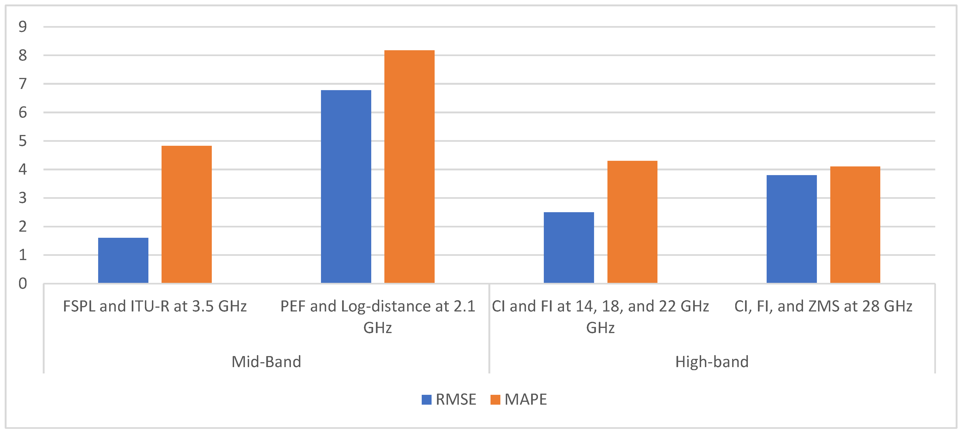
| [61] | 3.5 | Model fit, FSPL, and ITU-R | LOS and NLOS | Indoor | Conduction of large-scale fading, using an omnidirectional antenna and a spectrum analyzer under two different scenarios. | The FSPL overestimates path loss whereas the ITU-R model performed better, therefore recommended to be used. | It will be necessary to conduct extensive measurement campaigns across similar structures to obtain a representative model. |
| [62] | 28 | Grey model, 5GCM, 3GPP, METIS, and mmMAGIC | LOS and NLOS | Outdoor–urban | The suggested path loss model was tested against four 5G empirical models after being trained using measured path loss data. | In contrast to the linear regression model, it is discovered that the proposed model has a good prediction. | There is need to test the comparative analysis beyond the mean absolute error (MAE) |
| [48] | 14, 18, and 22 | CI and FI | LOS and NLOS | Indoor | Measurement campaigns were carried out to examine the models and path loss exponent (PLE). | The LoS comparison demonstrates that for the chosen frequency bands, the two models produce precise estimates that fit the actual measured data. | The impact of the materials surrounding the symmetry of the environment were not considered. |
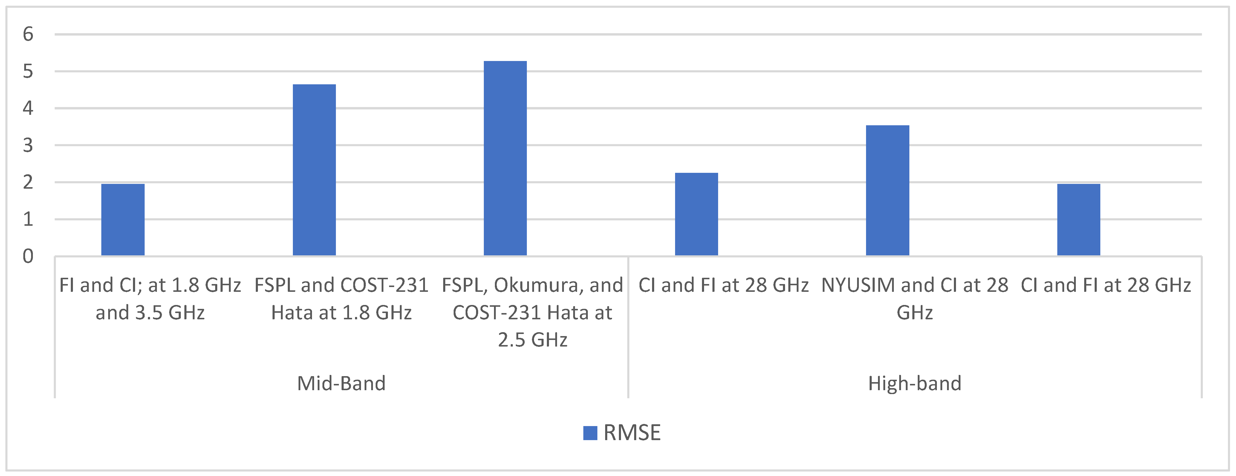
| [47] | 28 | CI, FI, and RMSE | LOS and NLOS | Outdoor–urban | Two 5G models were employed to evaluate the best path loss model. Additionally, five distinct path loss scenarios were analyzed during this process. | The FI model performed better with the lowest value of RMSE. | A live measurement campaign should be carried out for proper investigation |
| [66] | 26 | 3GPP, ABG, and CI | LOS and NLOS | Outdoor–rural | A comprehensive measurement campaign was conducted in two rural areas using a crane to assess path loss at transmite antenna heights of 30, 50, and 70 m. | The height of the cell site antenna appears to be a crucial design factor for network planning. | There is need to test the models in another frequency to know the stability at multiple frequencies. |
| [67] | 28 | FSPL, CIB, and CI | LOS | Outdoor–urban | Based on the data collected during measurement campaigns, some selected models were employed to look into the channel loss for the 5G system. | The CIB path loss model is suitable for the LOS scenarios as it aligns with the data from the environment. | There is a need to investigate the effect of return and mismatch losses along the feed line. |
| [68] | 28, 38, 60, 73, 100, and 120 | NYUSIM and CI | LOS and NLOS | Urban microcell | Large-scale simulation analysis on geometric parameters and environmental conditions for the proposed millimeter wave channels. | Geometric parameters and external factors affect the statistical channel modeling’s parameters. | For the suggested model’s performance to be verified and assessed, more experimental data are needed. |
| [69] | 1.8, 3.5, and 28 | FI and CI | LOS | Outdoor–urban | Modeling of path loss from wideband measurement campaign. | A guiding effect was noticed in the 1.8 GHz frequency band, which is not observed in other bands. | To check the stability of the models, a non-line-of-sight (NLoS) scenario should be taken into account. |
| [70] | PEF and Log-distance | LOS | Suburban | The “drive test” and “walk test” experiments were conducted to investigate propagation loss along distinct paths. | With an RMSE that was 1.4 dB lower, the suggested model performed better than the log-distance model. | The proposed model needs to be tested on other frequency bands to accurately determine the stability of the models. | |
| [71] | 28 | CI, FI, and ZMS | LOS and NLOS | Indoor | Simulation for all possible polarization at NLoS and LoS scenarios per meter over 47 m. | The straightforward model that is suggested, which only has one parameter called ZMS, can forecast expansive path loss across distance. | To develop a model that is representative, a comprehensive measuring campaign across comparable buildings will be necessary. |
| [42] | 1.8 | FSPL and COST-231 Hata | LOS | Urban | With the dataset gathered from drive tests, the proposed model was tuned using the magnetic optimization algorithm (MOA). | With a lower RMSE value, the proposed augmented model outperformed and was more representational of the data than its traditional counterparts. | The magnetic optimization algorithm that was used has deficiencies in handling non-linearity and may suffer from convergence issues to provide an accurate model. |
| [72] | 2.5 | FSPL, SUI, Okumura, and COST-231 Hata. | LOS | Urban | Five different empirical models were tested with actual data measurements to find the most performed model to predict path loss. | The COST-231 Hata model proved to be more suitable than the other chosen models, with a minimal RMSE of 5.27 dB. | The COST-231 Hata model needs to be fine-tuned to suit the special scenario of the urban environment that comprises old and modern buildings. |
| Reference | Freq. (GHz)/Scenario | ML. Algorithm | Input Features | Performance Indicators | Important Results | Limitations/Area of Improvement |
|---|---|---|---|---|---|---|
| [74] | 28/ Urban | CNN | Tx, Rx, floor plan image matrix | RMSE | The proposed model outperformed the chosen models, demonstrating a root mean square error of 8.59 dB. | To accurately determine the model stability, the result should be modeled with multiple parameters. |
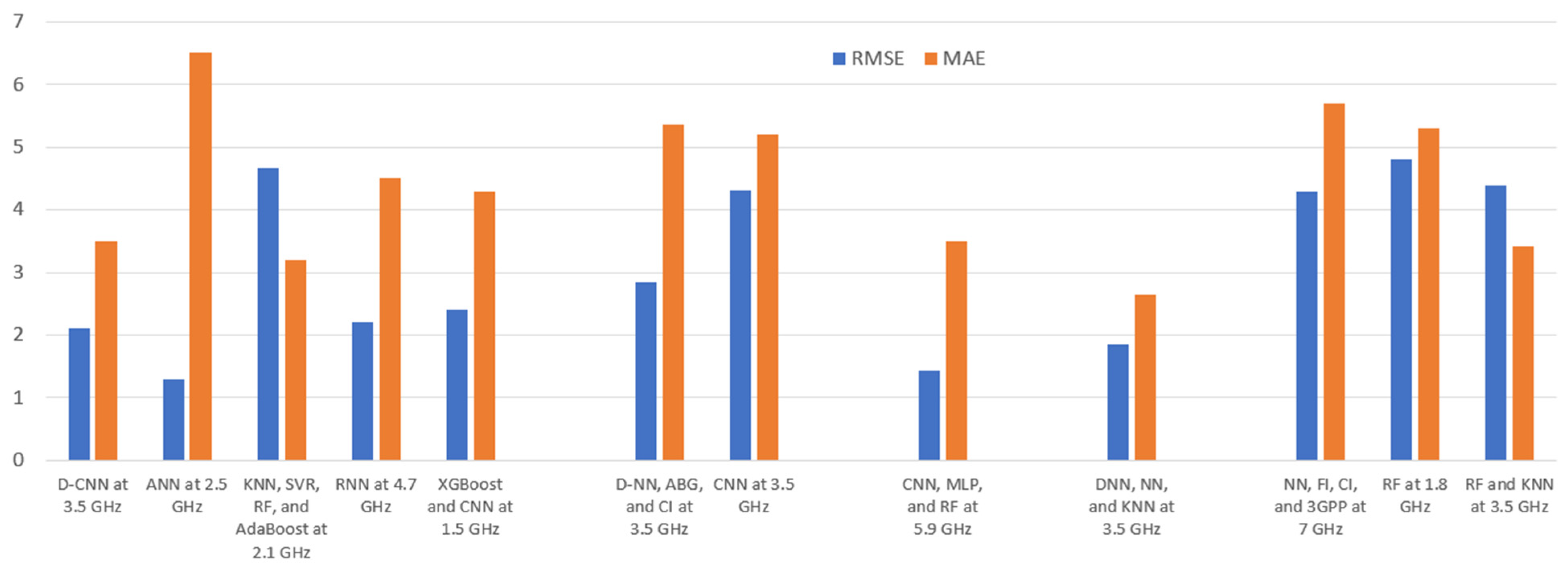
| [75] | 3.5/ Urban | D-CNN | Satellite image, pl exponent, and shadow factor | MSE | The results made public demonstrate a high degree of real-time channel parameter prediction accuracy. | In commercial environments with more impediments, the path loss model needs to be tested. |
| [76] | 28/ Urban | RF | Tx power, Tx antenna gain, terrain profile, and site coordinates | RMSE and cost time | This study recommends employing the RF model, as it was proven to be reliable with high accuracy. | There is a need to compare the proposed model with any of the widely used models in the same environment to test its validity. |
| [77] | 3.7/ Rural | ANN, RF, SVR, and B-kNN | Distance between Tx and Rx, Tx height, and Rx height | RMSE, ME, MAPE, MAE, and σ | The ML models outperformed the empirical ones with remarkably low RMSE on the order of 4.2 to 4.3 dB after a comparison between the proposed ML models and those of the chosen empirical models. | It only takes path loss and distance into consideration. Another important element that must be taken into consideration is frequency. |
| [78] | 28/ Indoor | CNN | LAMS images | RMSE | The suggested model solved the few-shot data problem and implemented path loss prediction in a smart factory. | There is a need to test the proposed model in a non-line-of-sight scenario to deduce its stability in the indoor environment. |
| [79] | 2.5/Suburban, Urban | ANN | 3D locations, frequency, transmitted and receiver power, antenna information, and feeder loss | AME, MAE, STD, and TR | These PL prediction models become more accurate and stable when environmental data are included, with unweighted rectangular environmental features performing better. | The suggested model’s viability needs to be examined in a commercial environment with a higher level of obstruction. |
| [80] | 28/Suburban, Urban | AE—CNN | GPS Tx and Rx coordinates, DE-LAMS image size, and Google map image matrix | RMSE | Modern deterministic and empirical techniques cannot match the proposed innovative AE-CNN path loss model in suburban environments. | Improvements must be made to the suggested model’s performance in the line-of-sight (LoS) situation. |
| [81] | 2.1/ Urban | KNN, SVR, RF, and AdaBoost | Vertical and horizontal coordinates (x,y) for FBS height | RMSE, MAE, and MAPE | The most accurate predictions came from the tree-based ensemble models, with AdaBoost achieving the lowest MAPE value of 2.72%. | Distinct scenarios should be examined for the comparative examination of the models. |
| [82] | 2.2, 4.7, and 26.4/Urban | RNN | Path loss and gate layer | RMSE | With an RMSE of 2dB, the suggested method outperformed the standard method for predicting path loss using LSTM, a type of RNN utilized in time series prediction. | To verify the performance of the suggested model at various frequencies, more performance indicators should be implemented. |
| [83] | 1.5/ Urban | XGBoost, CNN | Data in tabular form, pictures (Tr_to_R_area), and pseudo images. | MAE, MAPE, and RMSE | The proposed strategy produced superior results than prior fusion methods, with an MAE value of 3.07 dB as opposed to the 3.15 dB of the traditional bimodal approaches. | For the performance of the suggested model to be verified, more experimental data are needed. |
| [84] | 3.5/ Urban | D-NN, ABG, and CI | Tx height, Tx-Rx pair separation, and path profile. | RMSE | According to simulation data, the proposed model performs better than traditional models and has an accuracy of 72%. | There is a need to investigate the applicability of the proposed model in a commercial environment. |
| [85] | 2.5/ Urban | DL | 3D image | MAE, MAPE, and RMSE | It has been demonstrated that for lower transmitter heights, texture’s influence is more significant. The features are consistently provided by the SFTA algorithm. | It will be necessary to conduct an extensive measurement campaign to obtain a representable model. |
| [86] | 28/ Urban | 3D—CNN | 3D—LAMS image | RMSE | When the data were extracted into a 40 m square, the best performance was attained. | To know the stability at multiple frequencies, the result should be modeled with more input features. |
| [87] | 3.5/ Urban | CNN | Building height, image, and distance from Tx and Rx | RMSE | The region where the NN model’s estimation accuracy declined was concentrated close to Tx, according to the proposed CNN model, which was built using the same principle as the NN model. | To validate the performance of the suggested model at various frequencies, performance measures should go beyond RMSE. |
| [88] | 5.9/ Urban | MLP, CNN, and RF | Coordinates for Tx and Rx, the number of buildings on the path, the distances covered inside and outside of structures, the widths of the streets where Tx and Rx are located, and the separations between Tx and Rx from side corners | MAE, MAPE, and RMSE | RF performed better than the MLP model, which had a maximum RMSE value of 11 ns, among the machine learning models used to characterize the impacts of radio wave propagation in dynamic vehicle situations. | Testing the proposed model in an environment with more obstacles, such as a commercial one, is necessary. |
| [31] | 28/ Urban | LR, MLR1, and MLR2 | Distance between T and R, time delay, received power, RMS delay spread, azimuth and elevation AoDs, and elevation AoAs | MAE, MSE, RMSE, and R-squared | Prediction of the model for new communication scenarios with the reduction in the required number of measurements and complexity. | For the proposed model’s performance to be verified, more input features are needed. |
| [89] | 60/ Urban | CNN and MLP | 3D image | MAE, RMSE, and RMSLE | The suggested model, which utilizes building footprint and top-view photos to forecast path loss, was presented. | Training features from a physical measurement campaign are required to validate the performance of the model. |
| [90] | 3.5/ Urban | GLMs, NNs, and k-NN | Image, TX power, and coordinates of the transmitter | MAE | Simpler models with higher performance and lower computational cost are GLM and KNN. | More performance indicators should be used to validate each model’s performance for comparison. |
| [91] | 2.5/ Indoor | LR and ANN | Reflections of the ground, ceiling, and walls | MSE and MAE | With the lowest MSE and MAE values, the ANN model outperformed the linear model in terms of performance. | It just takes into account the surface of the reflection area. Another important factor that needs to be taken into account is obstruction. |
| [92] | 2.3/ Indoor | GPR, LG, and KNN | Received power, T-R separation distance, elevation, and azimuth AoD | MSE and MAE | A multi-dimensional GPR-based model that is capable of estimating path loss was proposed. | Varied environments need to be used to test the stability of the proposed model. |
| [93] | 7/ Urban | NN, FI, CI, WINNER II, and 3GPP | 3D distance between Tx and Rx, center frequency, Tx height, Rx height, latitude, longitude, and satellite image | RMSE | When compared to the selected traditional models, the proposed model provided superior accuracy in predicting path loss. | The model needs to be improved in the context of the environment with more obstructions. |
| [94] | 1.8/ Urban | RF | Cell distance, vertical angle, horizontal angle from Rx, total height of Tx, total height of Rx, road width, and height of nearby buildings | MAPE and RMSE | Employing hyperparameter tuning for the suggested model leads to enhanced predictive accuracy performance. | Exploratory data analysis (EDA) is important and should be improved on the available data. |
| [95] | 3.5/ Urban | RF | Geographical coordinates, distance, azimuth, and antenna gain | MAE and RMSE | The use of an RF model with the given attributes presents better prediction accuracy | Enhancing the model’s performance requires the inclusion of supplementary input features. |
Disclaimer/Publisher’s Note: The statements, opinions and data contained in all publications are solely those of the individual author(s) and contributor(s) and not of MDPI and/or the editor(s). MDPI and/or the editor(s) disclaim responsibility for any injury to people or property resulting from any ideas, methods, instructions or products referred to in the content. |
© 2023 by the authors. Licensee MDPI, Basel, Switzerland. This article is an open access article distributed under the terms and conditions of the Creative Commons Attribution (CC BY) license (https://creativecommons.org/licenses/by/4.0/).
Share and Cite
Shaibu, F.E.; Onwuka, E.N.; Salawu, N.; Oyewobi, S.S.; Djouani, K.; Abu-Mahfouz, A.M. Performance of Path Loss Models over Mid-Band and High-Band Channels for 5G Communication Networks: A Review. Future Internet 2023, 15, 362. https://doi.org/10.3390/fi15110362
Shaibu FE, Onwuka EN, Salawu N, Oyewobi SS, Djouani K, Abu-Mahfouz AM. Performance of Path Loss Models over Mid-Band and High-Band Channels for 5G Communication Networks: A Review. Future Internet. 2023; 15(11):362. https://doi.org/10.3390/fi15110362
Chicago/Turabian StyleShaibu, Farouq E., Elizabeth N. Onwuka, Nathaniel Salawu, Stephen S. Oyewobi, Karim Djouani, and Adnan M. Abu-Mahfouz. 2023. "Performance of Path Loss Models over Mid-Band and High-Band Channels for 5G Communication Networks: A Review" Future Internet 15, no. 11: 362. https://doi.org/10.3390/fi15110362
APA StyleShaibu, F. E., Onwuka, E. N., Salawu, N., Oyewobi, S. S., Djouani, K., & Abu-Mahfouz, A. M. (2023). Performance of Path Loss Models over Mid-Band and High-Band Channels for 5G Communication Networks: A Review. Future Internet, 15(11), 362. https://doi.org/10.3390/fi15110362