
Seeing through Wavy Water–Air Interface: A Restoration Model for Instantaneous Images Distorted by Surface Waves

Abstract
:1. Introduction
2. Optical Analysis of Imaging through Refractive Media
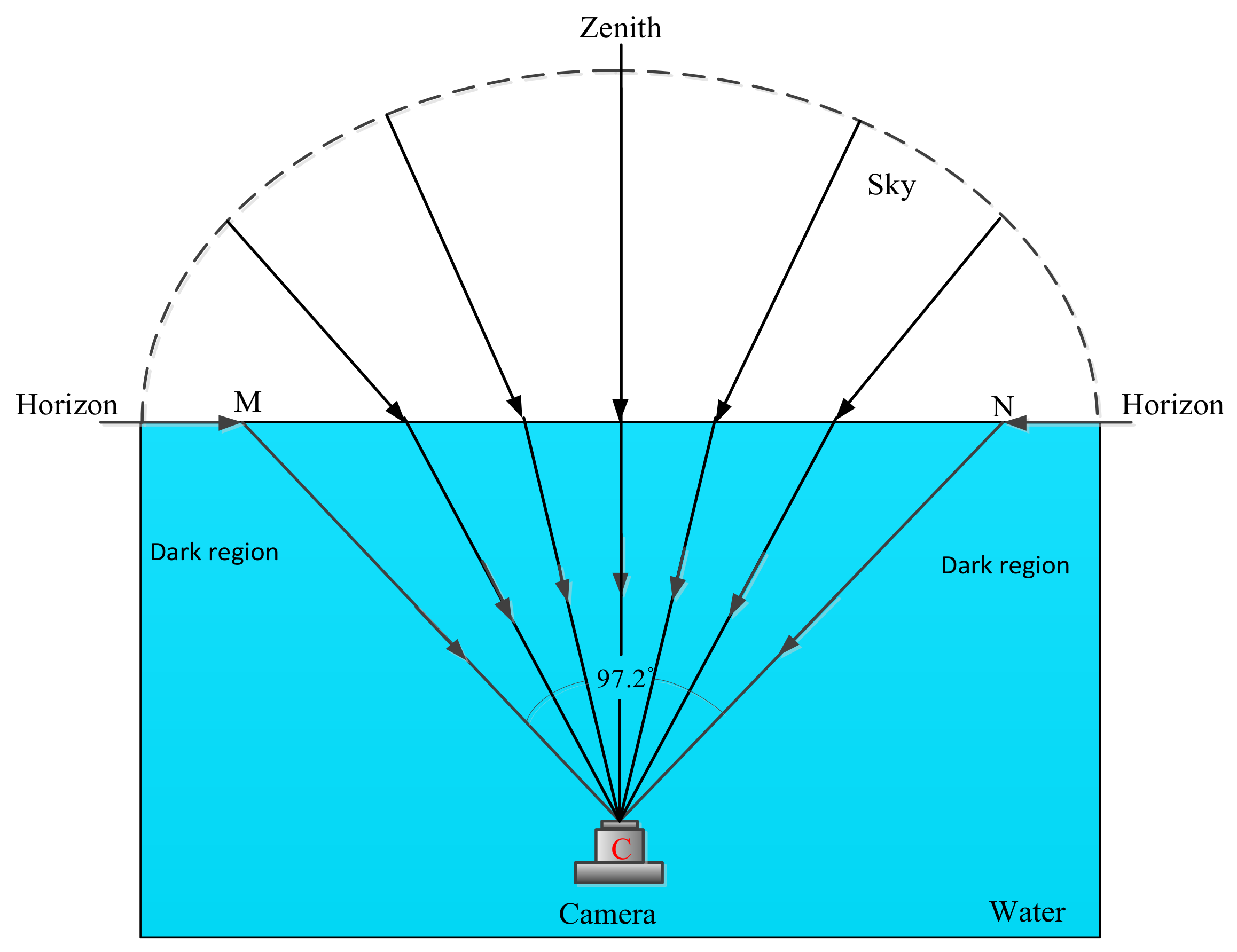
2.1. Snell’s Window
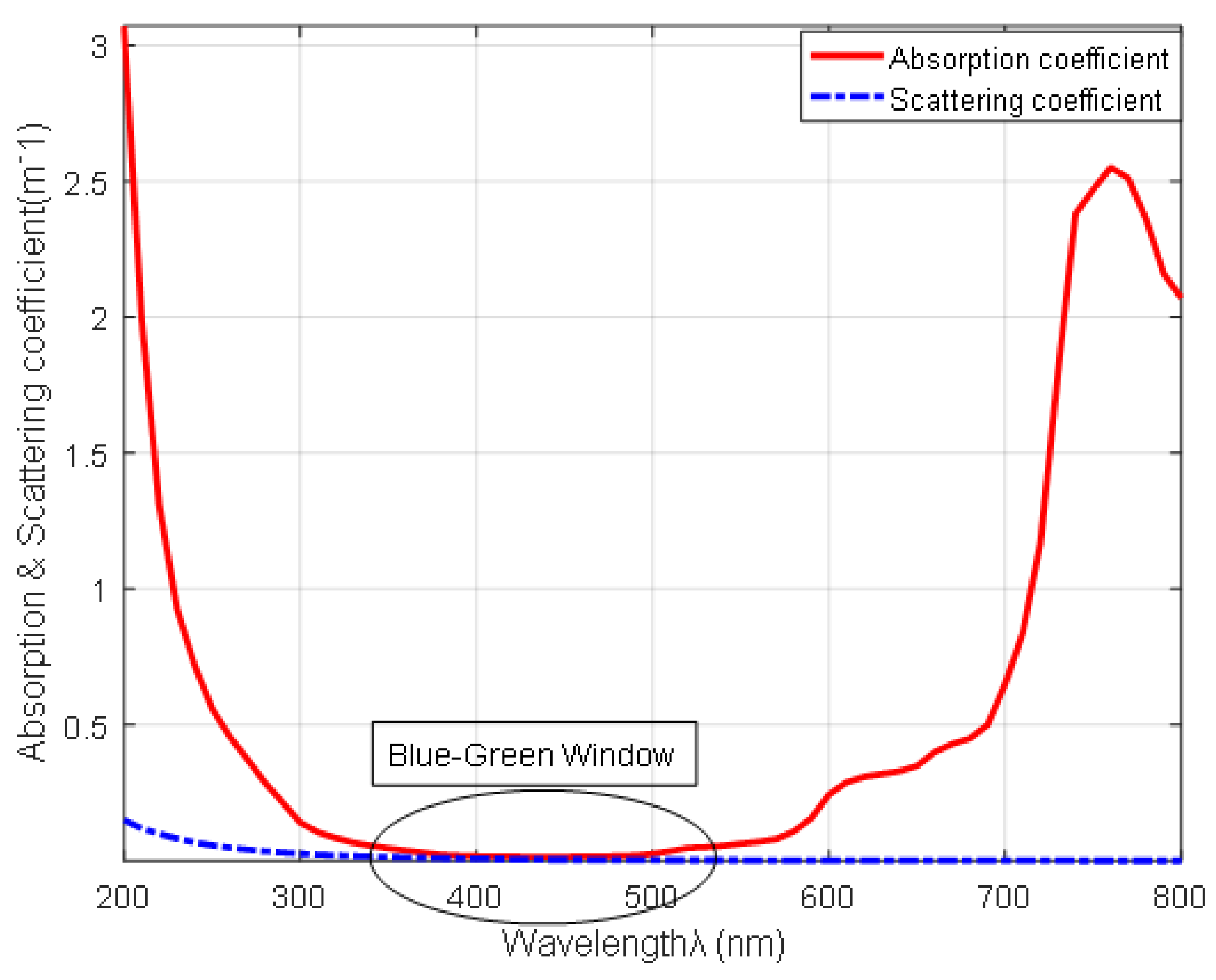
2.2. Optical Properties of Sea Water
3. Materials and Methods
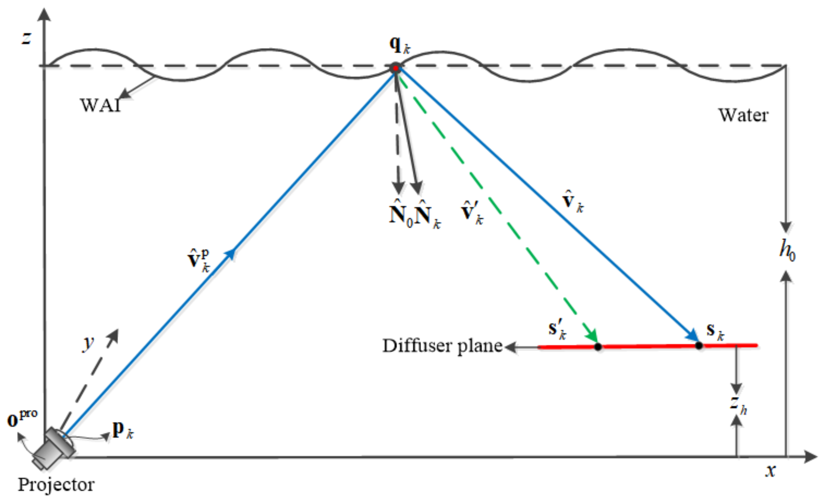
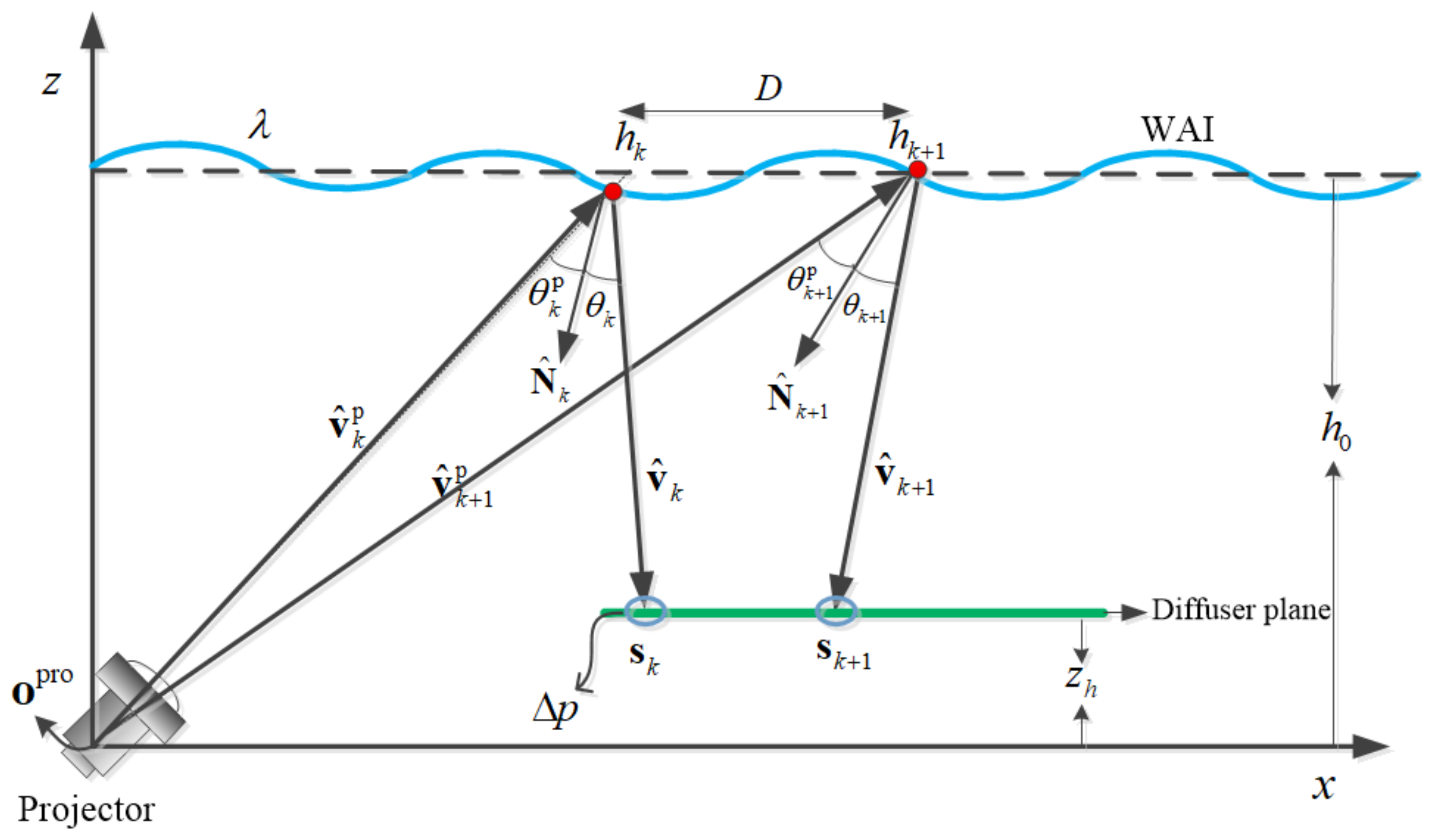
3.1. Model Descriptions
3.2. WAI Reconstruction Algorithm Based on Finite Difference
3.2.1. Sampling of WAI Normals
3.2.2. Reconstruction of the WAI
3.3. Image Restoration Algorithm through Ray Tracing
4. Limitations
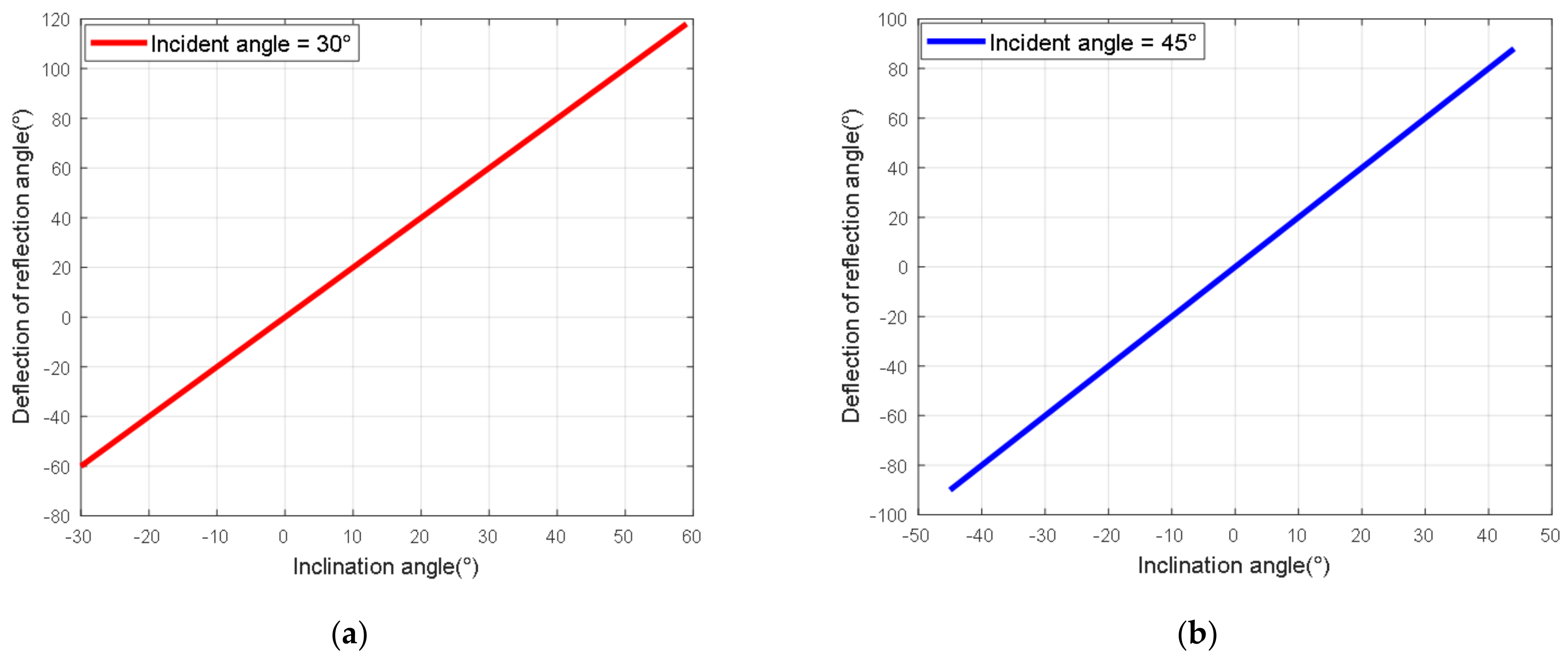
4.1. Sensitivity to Variations in for Structured Light
4.2. Resolution Analysis
5. Results
5.1. System Parameters
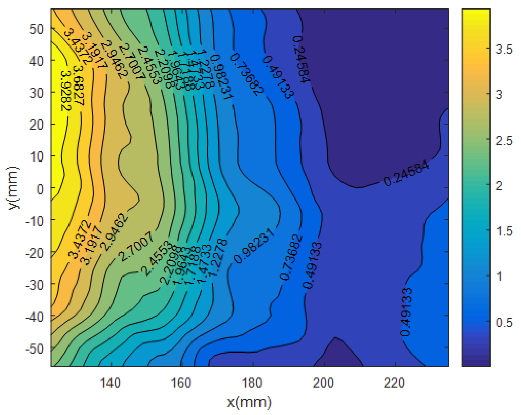
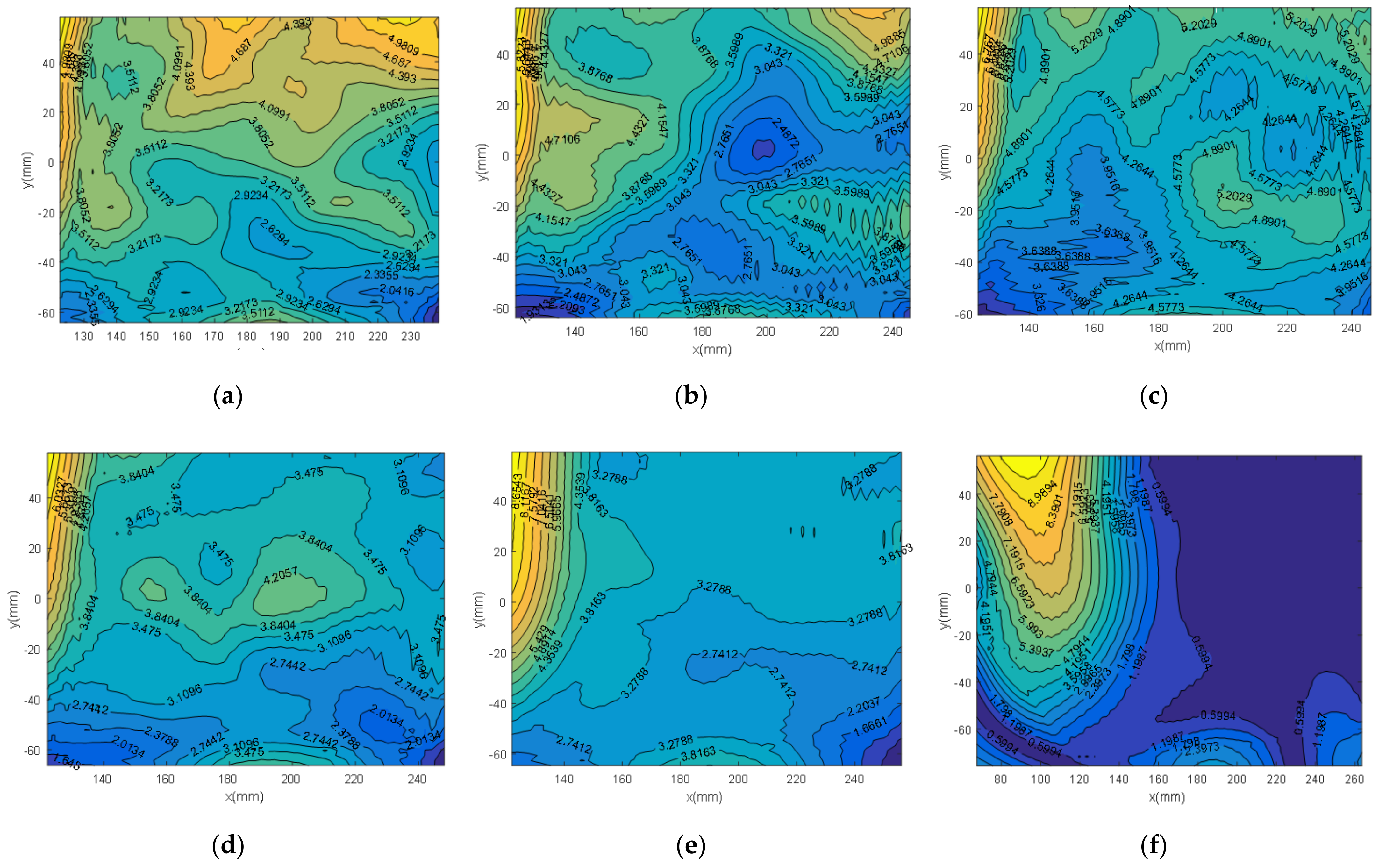
5.2. WAI Reconstruction
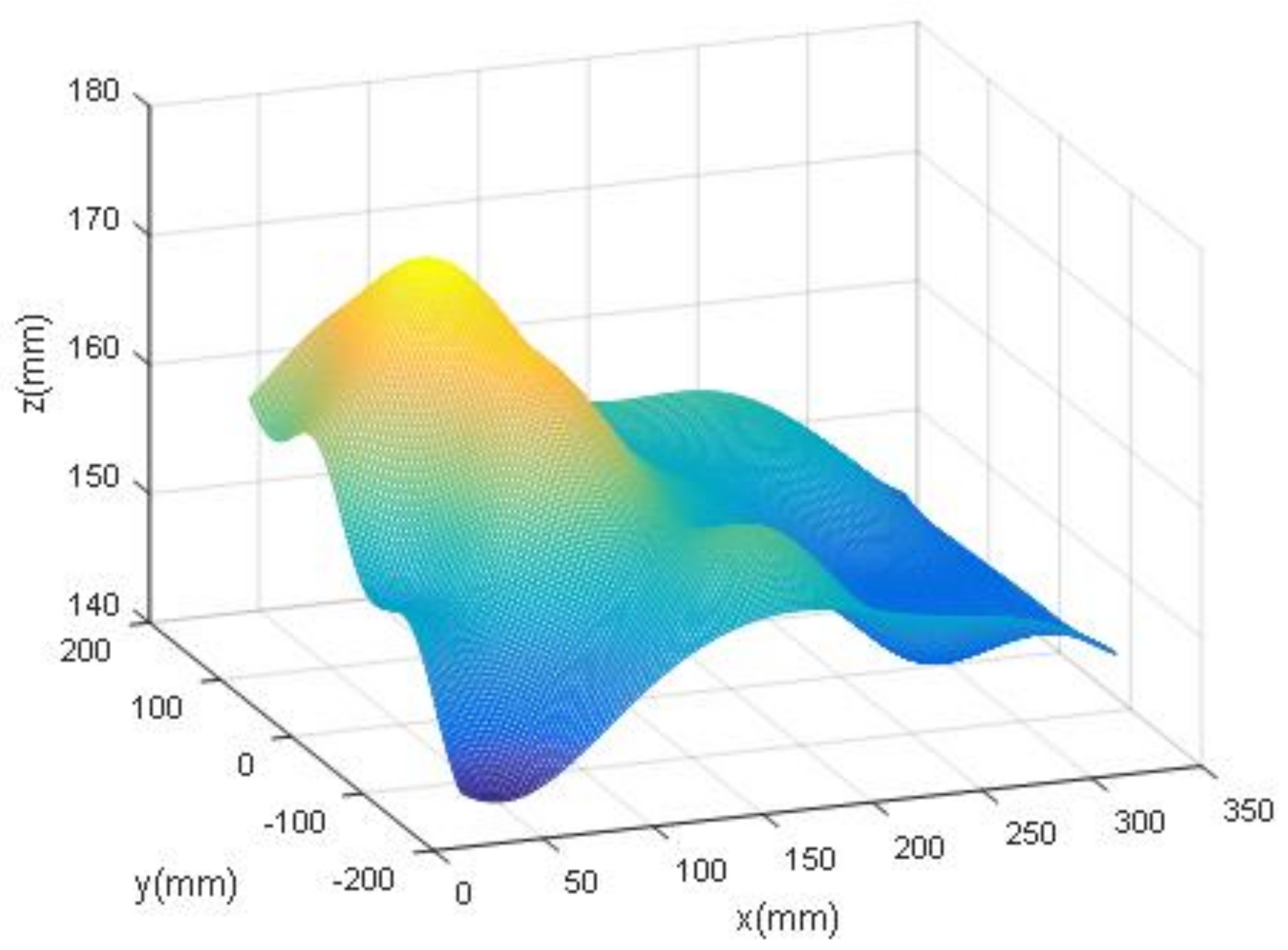
5.2.1. WAI Simulation
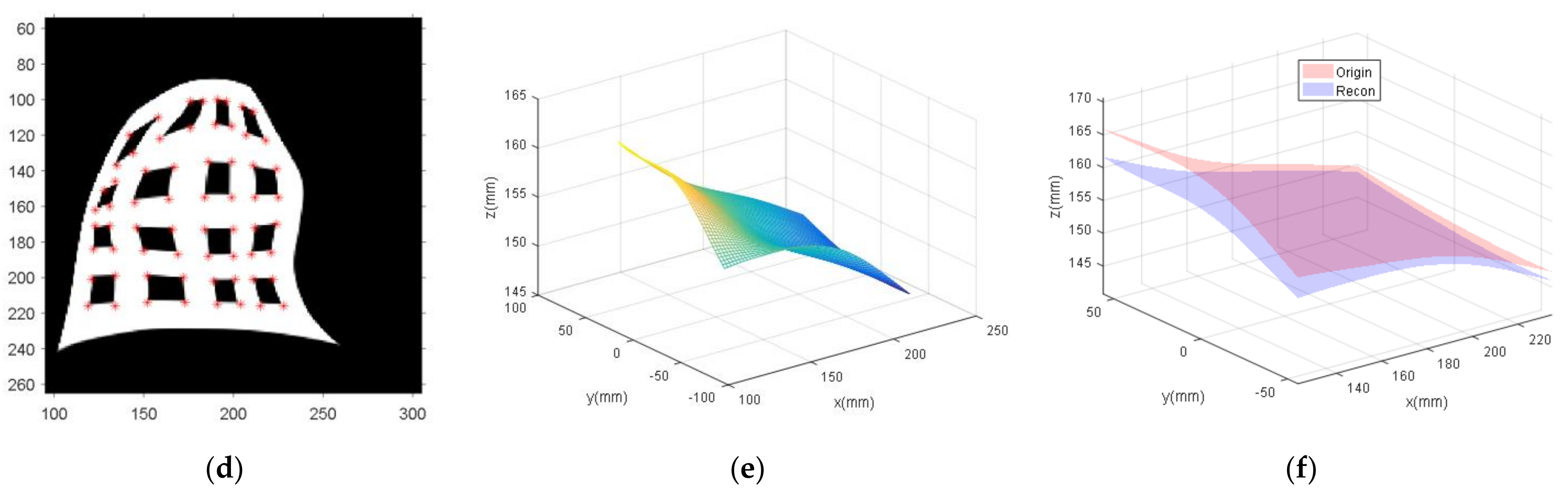
5.2.2. Reconstruction of the WAI
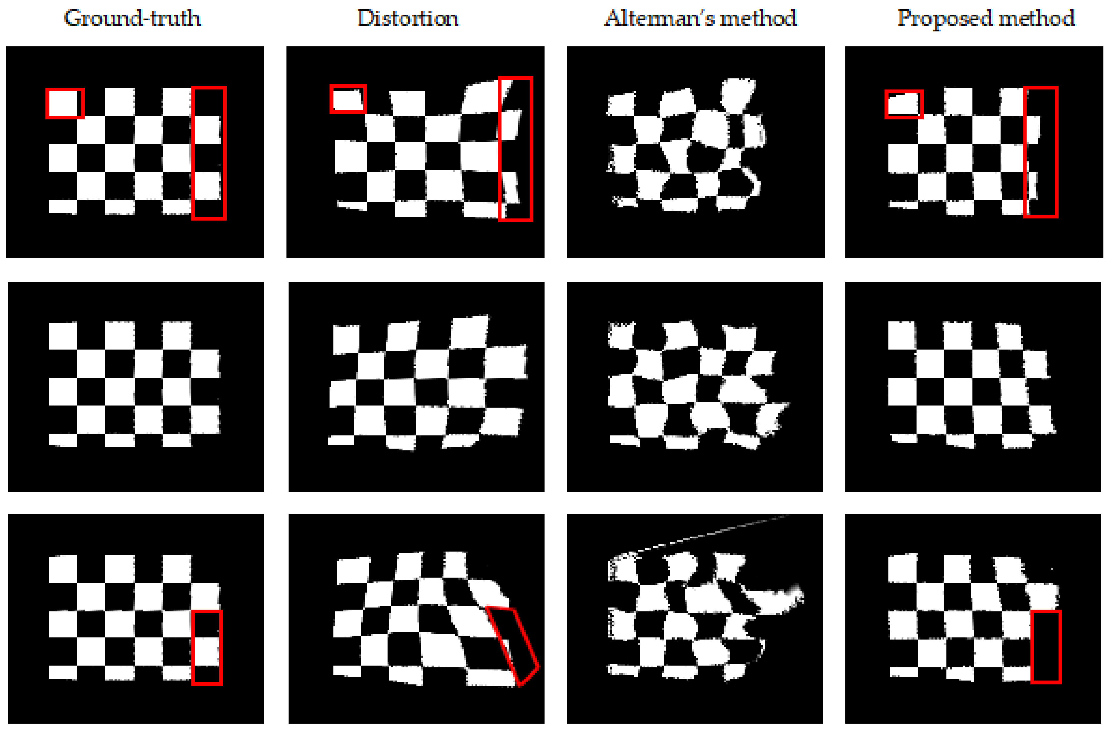
5.2.3. Comparative Analysis with Alterman’s Method
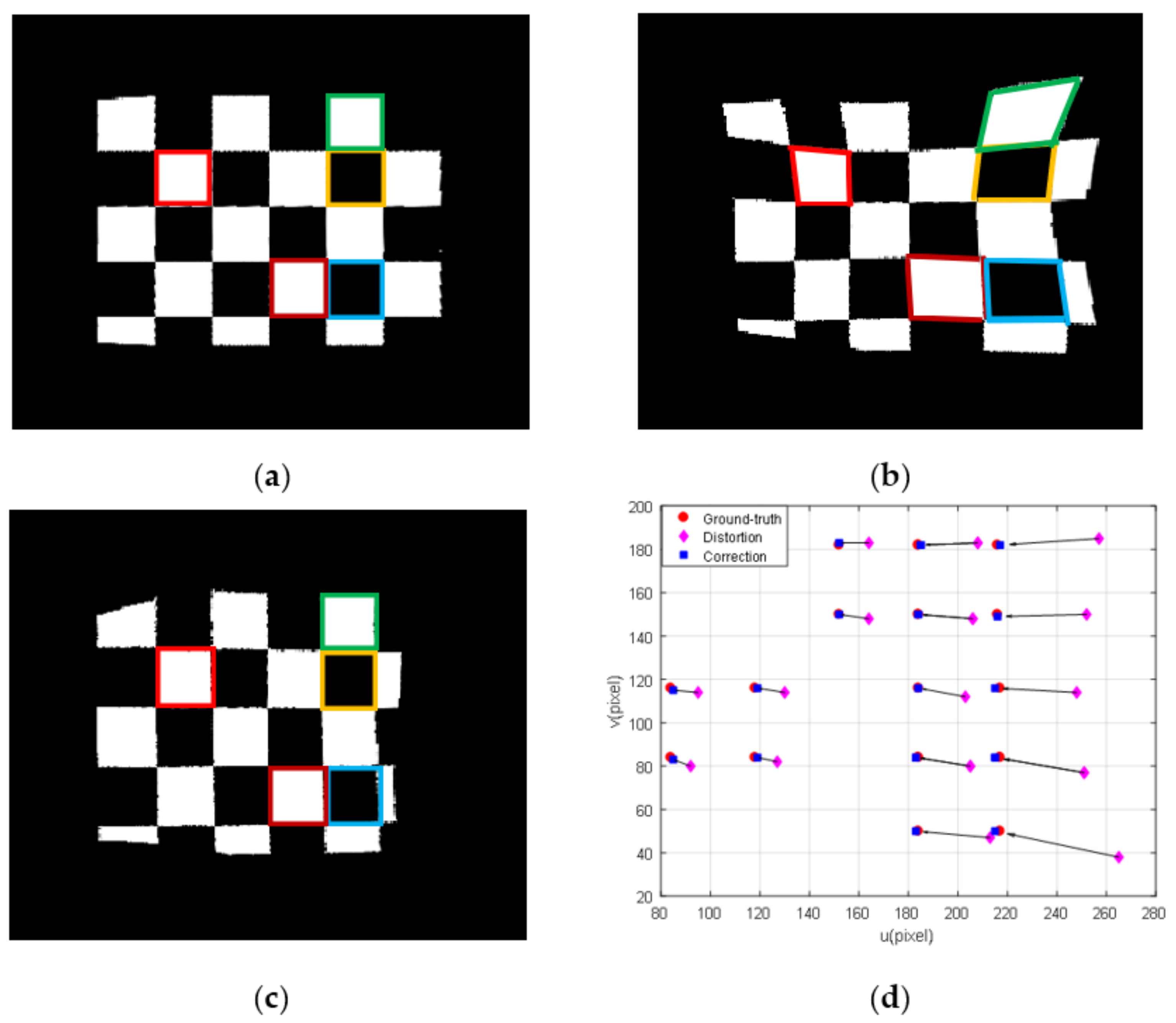
5.3. Image Restoration
5.3.1. Image Quality Metrics
5.3.2. Results of Quantitative Analysis
6. Conclusions
Author Contributions
Funding
Data Availability Statement
Conflicts of Interest
References
- Alterman, M.; Schechner, Y.Y.; Perona, P.; Shamir, J. Detecting motion through dynamic refraction. IEEE Trans. Pattern Anal. Mach. Intell. 2012, 35, 245–251. [Google Scholar] [CrossRef] [PubMed] [Green Version]
- Zhang, R.; He, D.; Li, Y.; Bao, X. Synthetic imaging through wavy water surface with centroid evolution. Opt. Express 2018, 26, 26009–26019. [Google Scholar] [CrossRef] [PubMed]
- Molkov, A.A.; Dolin, L.S. The Snell’s window image for remote sensing of the upper sea layer: Results of practical application. J. Mar. Sci. Eng. 2019, 7, 70. [Google Scholar] [CrossRef] [Green Version]
- Cai, C.; Meng, H.; Qiao, R.; Wang, F. Water–air imaging: Distorted image reconstruction based on a twice registration algorithm. Mach. Vis. Appl. 2021, 32, 64. [Google Scholar] [CrossRef]
- Tian, Y.; Narasimhan, S.G. Seeing through water: Image restoration using model-based tracking. In Proceedings of the IEEE 12th International Conference on Computer Vision, Kyoto, Japan, 27 September–4 October 2009. [Google Scholar]
- Tian, Y.; Narasimhan, S.G. Globally optimal estimation of nonrigid image distortion. Int. J. Comput. Vis. 2012, 98, 279–302. [Google Scholar] [CrossRef] [Green Version]
- Halder, K.K.; Tahtali, M.; Anavatti, S.G. An Artificial Neural Network Approach for Underwater Warp Prediction. In Proceedings of the 8th Hellenic Conference on Artificial Intelligence, Ioannina, Greece, 15–17 May 2014; Springer: Cham, Switzerland, 2014; pp. 384–394. [Google Scholar]
- Seemakurthy, K.; Rajagopalan, A.N. Deskewing of Underwater Images. IEEE Trans. Image Process. 2015, 24, 1046–1059. [Google Scholar] [CrossRef]
- Li, Z.; Murez, Z.; Kriegman, D.; Ramamoorthi, R.; Chandraker, M. Learning to see through turbulent water In Proceedings of the 2018 IEEE Winter Conference on Applications of Computer Vision (WACV) (2018). Lake Tahoe, NV, USA, 12–15 March 2018; pp. 512–520. [Google Scholar]
- James, J.G.; Agrawal, P.; Rajwade, A. Restoration of Non-rigidly Distorted Underwater Images using a Combination of Compressive Sensing and Local Polynomial Image Representations. In Proceedings of the IEEE International Conference on Computer Vision, Seoul, Korea, 27 October–2 November 2019. [Google Scholar]
- James, J.G.; Rajwade, A. Fourier Based Pre-Processing for Seeing through Water. In Proceedings of the IEEE Winter Conference on Applications of Computer Vision, Snowmass, CO, USA, 1–5 March 2020. [Google Scholar]
- Thapa, S.; Li, N.; Ye, J. Learning to Remove Refractive Distortions from Underwater Images. In Proceedings of the IEEE/CVF International Conference on Computer Vision, Montreal, BC, Canada, 11–17 October 2021; pp. 5007–5016. [Google Scholar]
- Cox, C.; Munk, W. Slopes of the sea surface deduced from photographs of sun glitter. Bull. Scripps Inst. Oceanogr. 1956, 6, 401–479. [Google Scholar]
- Zapevalov, A.; Pokazeev, K.; Chaplina, T. Simulation of the Sea Surface for Remote Sensing; Springer: Cham, Switzerland, 2021. [Google Scholar]
- Milder, D.M.; Carter, P.W.; Flacco, N.L.; Hubbard, B.E.; Jones, N.M.; Panici, K.R.; Platt, B.D.; Potter, R.E.; Tong, K.W.; Twisselmann, D.J. Reconstruction of through-surface underwater imagery. Waves Random Complex Media 2006, 16, 521–530. [Google Scholar] [CrossRef]
- Schultz, H.; Corrada-Emmanuel, A. System and Method for Imaging through an Irregular Water Surface. U.S. Patent 7,630,077, 8 December 2009. [Google Scholar]
- Levin, I.M.; Savchenko, V.V.; Osadchy, V.J. Correction of an image distorted by a wavy water surface: Laboratory experiment. Appl. Opt. 2008, 47, 6650–6655. [Google Scholar] [CrossRef]
- Weber, W.L. Observation of underwater objects through glitter parts of the sea surface. Radiophys. Quantum Electron. 2005, 48, 34–47. [Google Scholar] [CrossRef]
- Dolin, L.S.; Luchinin, A.G.; Turlaev, D.G. Algorithm of reconstructing underwater object images distorted by surface waving. Izv. Atmos. Ocean. Phys. 2004, 40, 756–764. [Google Scholar]
- Luchinin, A.G.; Dolin, L.S.; Turlaev, D.G. Correction of images of submerged objects on the basis of incomplete information about surface roughness. Izv. Atmos. Ocean. Phys. 2005, 41, 247–252. [Google Scholar]
- Dolin, L.; Gilbert, G.; Levin, I.; Luchini, A. Theory Imaging Through Wavy Sea Surf; IAP RAS: Nizhny Novgorod, Russia, 2006. [Google Scholar]
- Dolin, L.S.; Luchinin, A.G.; Titov, V.I.; Turlaevm, D.G. Correcting images of underwater objects distorted by sea surface roughness. In Current Research on Remote Sensing, Laser Probing, and Imagery in Natural Waters; Society of Photo-Optical Instrumentation Engineers: Bellingham, DC, USA, 2007; Volume 66150, pp. 181–192. [Google Scholar]
- Alterman, M.; Swirski, Y.; Schechner, Y.Y. STELLA MARIS: Stellar marine refractive imaging sensor. In Proceedings of the 2014 IEEE International Conference on Computational Photography (ICCP), Santa Clara, CA, USA, 2–4 May 2014. [Google Scholar]
- Alterman, M.; Schechner, Y.Y. 3D in Natural Random Refractive Distortions; Javidi, B., Son, J.-Y., Eds.; International Society for Optics and Photonics: Bellingham, DC, USA, 2016; Volume 9867. [Google Scholar]
- Gardashov, R.H.; Gardashov, E.R.; Gardashova, T.H. Recovering the instantaneous images of underwater objects distorted by surface waves. J. Mod. Opt. 2021, 68, 19–28. [Google Scholar] [CrossRef]
- Suiter, H.; Flacco, N.; Carter, P.; Tong, K.; Ries, R.; Gershenson, M. Optics near the snell angle in a water-to-air change of medium. In Proceedings of the OCEANS 2007, Vancouver, BC, Canada, 29 September–4 October 2007; IEEE: Piscataway Township, NJ, USA, 2008. [Google Scholar]
- Lynch, D.K. Snell’s window in wavy water. Appl. Opt. 2015, 54, B8–B11. [Google Scholar] [CrossRef] [Green Version]
- Gabriel, C.; Khalighi, M.-A.; Bourennane, S.; Leon, P.; Rigaud, V. Channel modeling for underwater optical communication. In Proceedings of the 2011 IEEE GLOBECOM Workshops (GC Wkshps), Houston, TX, USA, 5–9 December 2011; IEEE: Piscataway Township, NJ, USA, 2011. [Google Scholar]
- Martin, M.; Esemann, T.; Hellbrück, H. Simulation and evaluation of an optical channel model for underwater communication. In Proceedings of the 10th International Conference on Underwater Networks & Systems, Arlington, VA, USA, 22–24 October 2015. [Google Scholar]
- Ali Mazin, A.A. Characteristics of optical channel for underwater optical wireless communication based on visible light. Aust. J. Basic Appl. Sci. 2015, 9, 437–445. [Google Scholar]
- Morel, A.; Gentili, B.; Claustre, H.; Babin, M.; Bricaud, A.; Ras, J.; Tièche, F. Optical properties of the “clearest” natural waters. Limnol. Oceanogr. 2007, 52, 217–229. [Google Scholar] [CrossRef]
- Born, M.; Wolf, E. Principles of Optics: Electromagnetic Theory of Propagation, Interference and Diffraction of Light; Elsevier: Amsterdam, The Netherlands, 2013. [Google Scholar]
- Sonka, M.; Hlavac, V.; Boyle, R. Image Processing, Analysis, and Machine Vision; Cengage Learning: Boston, MA, USA, 2014. [Google Scholar]
- Hartley, R.; Zisserman, A. Multiple View Geometry in Computer Vision; Cambridge University Press: Cambridge, UK, 2003. [Google Scholar]
- Ma, C.; Sun, Y.; Ao, J.; Jian, B.; Qin, F. A Centroid-Based Corner Detection Method for Structured Light. CN113409334A, 17 September 2021. [Google Scholar]
- Richard, L.; Burden, J.; Faires, D.; Annette, M.B. Numerical Analysis; Cengage Learning: Boston, MA, USA, 2015. [Google Scholar]
- Levenberg, K. A method for the solution of certain non-linear problems in least squares. Q. Appl. Math. 1944, 2, 164–168. [Google Scholar] [CrossRef] [Green Version]
- Gao, S.; Gruev, V. Bilinear and bicubic interpolation methods for division of focal plane polarimeters. Opt. Express 2011, 19, 26161–26173. [Google Scholar] [CrossRef]
- Jian, B. A Restoration Model for the Instantaneous Images Distorted by Surface Waves, version 2022. Available online: https://doi.org/10.6084/m9.figshare.20264520.v2 (accessed on 7 July 2022).
- Longuet-Higgins, M.S.; Stewart, R.W. Radiation stresses in water waves; a physical discussion, with applications. Deep.-Sea Res. Oceanogr. Abstr. 1964, 11, 529–562. [Google Scholar] [CrossRef]
- Neumann, G. On Ocean Wave Spectra and a New Method of Forecasting Wind-Generated Sea; Coastal Engineering Research Center: Vicksburg, MS, USA, 1953. [Google Scholar]
- Mitsuyasu, H.; Tasai, F.; Suhara, T.; Mizuno, S.; Ohkusu, M.; Honda, T.; Rikiishi, K. Observations of the directional spectrum of ocean WavesUsing a cloverleaf buoy. J. Phys. Oceanogr. 1975, 5, 750–760. [Google Scholar] [CrossRef] [Green Version]
- Hasselmann, K.; Barnett, T.P.; Bouws, E.; Carlson, H. Measurements of wind-wave growth and swell decay during the Joint North Sea Wave Project (JONSWAP). Ergaenzungsheft Zur Dtsch. Hydrogr. Z. Reihe A 1973, 12, 1–95. [Google Scholar]
- Poser, S.W. Applying Elliot Wave Theory Profitably; John Wiley & Sons: New York, NY, USA, 2003; Volume 169. [Google Scholar]
- Willard, J.P., Jr.; Moskowitz, L. A proposed spectral form for fully developed wind seas based on the similarity theory of SA Kitaigorodskii. J. Geophys. Res. 1964, 69, 5181–5190. [Google Scholar]
- Quan, H.T.; Ghanbari, M. Scope of validity of PSNR in image/video quality assessment. Electron. Lett. 2008, 44, 800–801. [Google Scholar]
- Hore, A.; Ziou, D. Image quality metrics: PSNR vs. SSIM. In Proceedings of International Conference on Pattern Recognition (ICPR), Istanbul, Turkey, 23–26 August 2010. [Google Scholar]
- Efros, A.; Isler, V.; Shi, J.; Visontai, M. Seeing through Water. In Advances in Neural Information Processing Systems; MIT Press: Cambridge, MA, USA, 2005; pp. 393–400. [Google Scholar]
- Wen, Z.; Lambert, A.; Fraser, D.; Li, H. Bispectral analysis and recovery of images distorted by a moving water surface. Appl. Opt. 2010, 49, 6376–6384. [Google Scholar] [CrossRef]
- Kanaev, A.V.; Hou, W.; Woods, S. Multi-frame underwater image restoration. In Electro-Optical and Infrared Systems: Technology and Applications VIII; International Society for Optics and Photonics: Bellingham, DC, USA, 2011. [Google Scholar]
- Kanaev, A.V.; Hou, W.; Restaino, S.R.; Matt, S.; Gładysz, S. Correction methods for underwater turbulence degraded imaging. In SPIE Remote Sensing; International Society for Optics and Photonics: Bellingham, DC, USA, 2014. [Google Scholar]
- Boyer, K.L.; Kak, A.C. Color-Encoded Structured Light for Rapid Active Ranging. IEEE Trans. Pattern Anal. Mach. Intell. 1987, PAMI-9, 14–28. [Google Scholar] [CrossRef]
- Barron, J.; David, L.; Fleet, J.; Beauchemin, S.S. Performance of optical flow techniques. Int. J. Comput. Vis. 1994, 12, 43–77. [Google Scholar] [CrossRef]


| System Parameters | Projector | Camera v | Camera s |
|---|---|---|---|
| CCD/LCD size | mm | mm | mm |
| Image resolution | |||
| 4.2 mm | 3.0 mm | 2.0 mm | |
| Rotation matrix | |||
| Translation vector |
| SSIM (H) | MSE (L) | PSNR (H) | |||||||
|---|---|---|---|---|---|---|---|---|---|
| Data 1 | Data 2 | Data 3 | Data 1 | Data 2 | Data 3 | Data 1 | Data 2 | Data 3 | |
| Distortion | 0.5584 | 0.6558 | 0.6140 | 0.1367 | 0.0653 | 0.0914 | 8.6414 | 11.8538 | 10.3925 |
| Alterman [23] | 0.6814 | 0.6784 | 0.6270 | 0.0520 | 0.0441 | 0.0514 | 12.8389 | 13.5571 | 12.8878 |
| Proposed method | 0.7630 | 0.7877 | 0.7434 | 0.0317 | 0.0461 | 0.0297 | 15.00 | 13.4651 | 15.2656 |
Publisher’s Note: MDPI stays neutral with regard to jurisdictional claims in published maps and institutional affiliations. |
© 2022 by the authors. Licensee MDPI, Basel, Switzerland. This article is an open access article distributed under the terms and conditions of the Creative Commons Attribution (CC BY) license (https://creativecommons.org/licenses/by/4.0/).
Share and Cite
Jian, B.; Ma, C.; Zhu, D.; Sun, Y.; Ao, J. Seeing through Wavy Water–Air Interface: A Restoration Model for Instantaneous Images Distorted by Surface Waves. Future Internet 2022, 14, 236. https://doi.org/10.3390/fi14080236
Jian B, Ma C, Zhu D, Sun Y, Ao J. Seeing through Wavy Water–Air Interface: A Restoration Model for Instantaneous Images Distorted by Surface Waves. Future Internet. 2022; 14(8):236. https://doi.org/10.3390/fi14080236
Chicago/Turabian StyleJian, Bijian, Chunbo Ma, Dejian Zhu, Yixiao Sun, and Jun Ao. 2022. "Seeing through Wavy Water–Air Interface: A Restoration Model for Instantaneous Images Distorted by Surface Waves" Future Internet 14, no. 8: 236. https://doi.org/10.3390/fi14080236
APA StyleJian, B., Ma, C., Zhu, D., Sun, Y., & Ao, J. (2022). Seeing through Wavy Water–Air Interface: A Restoration Model for Instantaneous Images Distorted by Surface Waves. Future Internet, 14(8), 236. https://doi.org/10.3390/fi14080236