
Analytical Modeling and Empirical Analysis of Binary Options Strategies


Abstract
1. Introduction
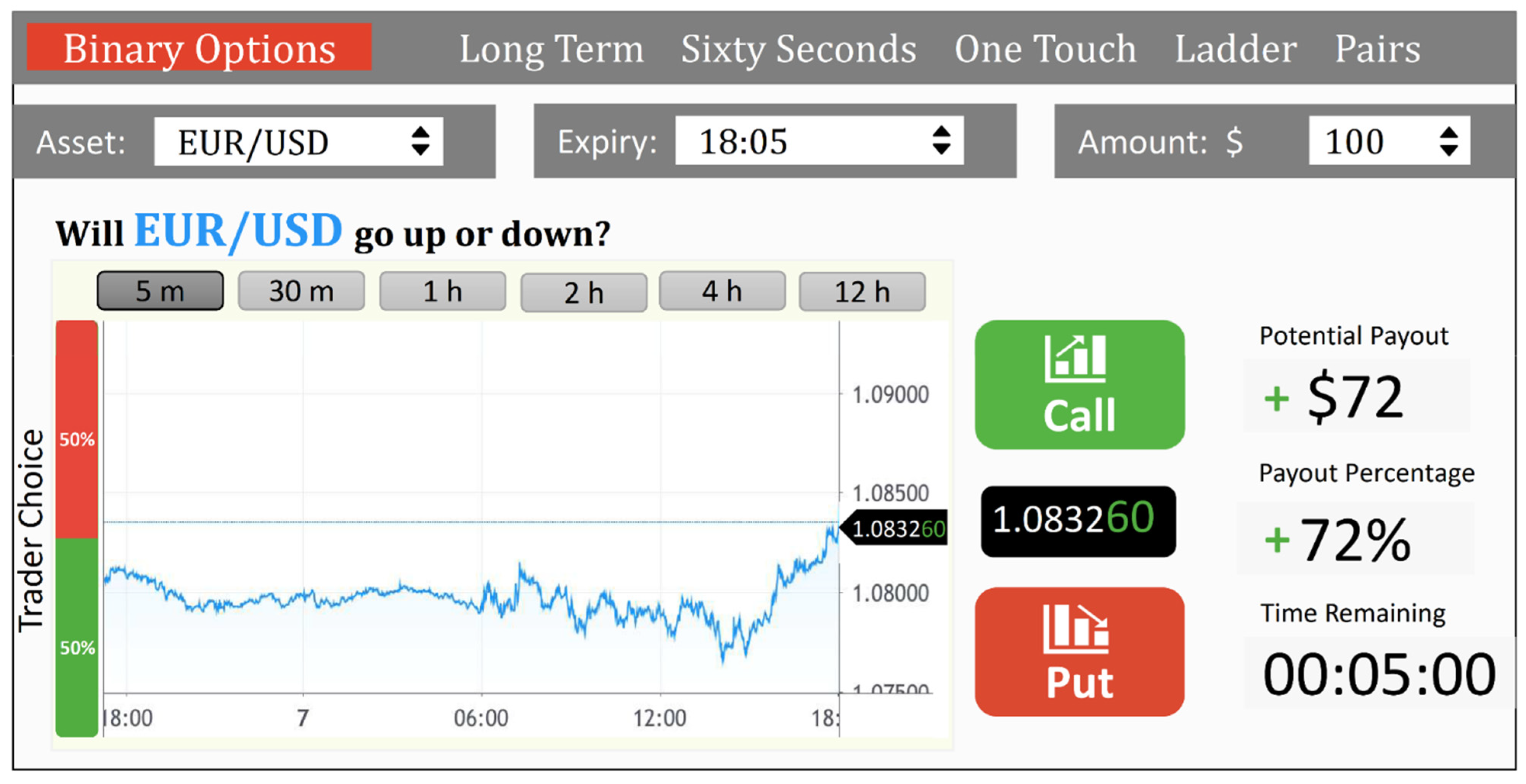
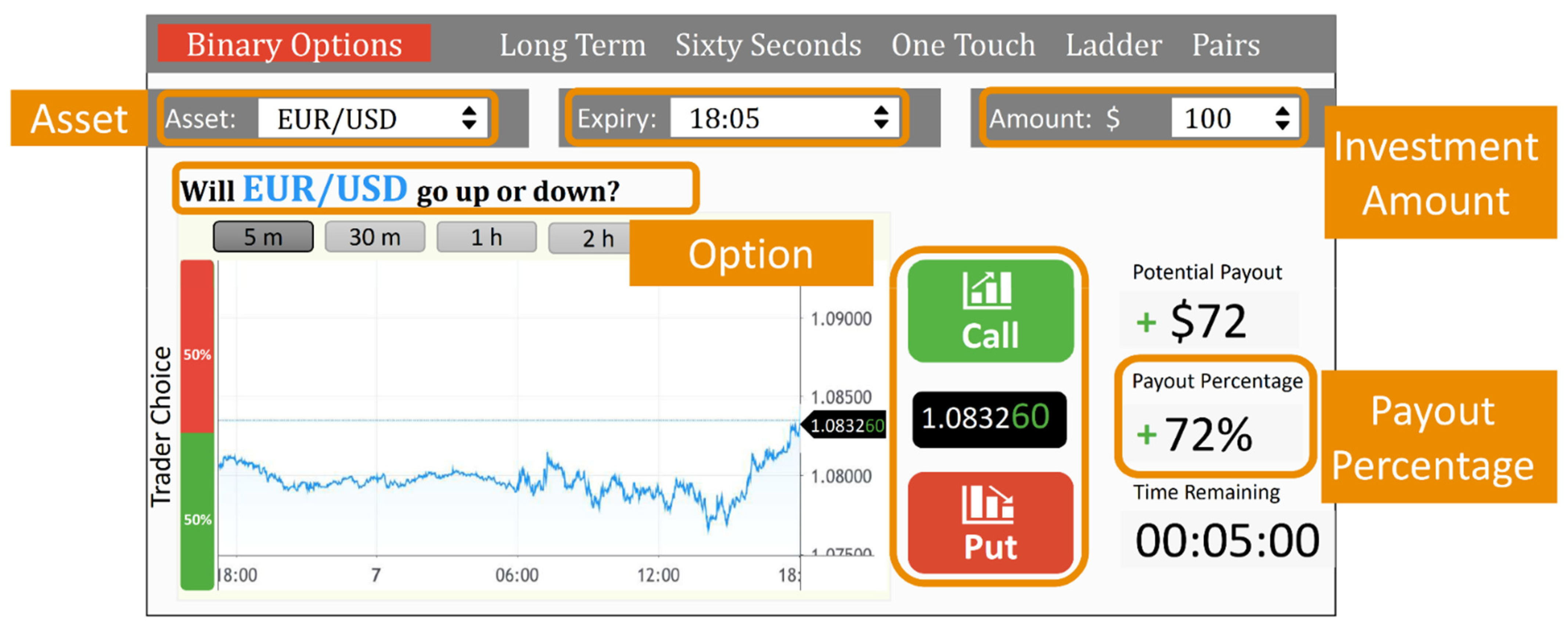
1.1. Binary Options
1.2. Literature Review Methodology
1.3. Literature Review
1.3.1. Exotic and Binary Options
1.3.2. Operational Mechanisms
1.3.3. Trading Algorithms
1.3.4. Options Pricing
1.3.5. Portfolio Management
1.3.6. Risks and Mitigation
1.4. Research Motivation, Design, and Contribution
1.4.1. Motivation
1.4.2. Design
1.4.3. Contributions
2. Materials and Methods
2.1. Monte Carlo Simulation
2.2. Statistical Measures
2.3. Visual Analytics
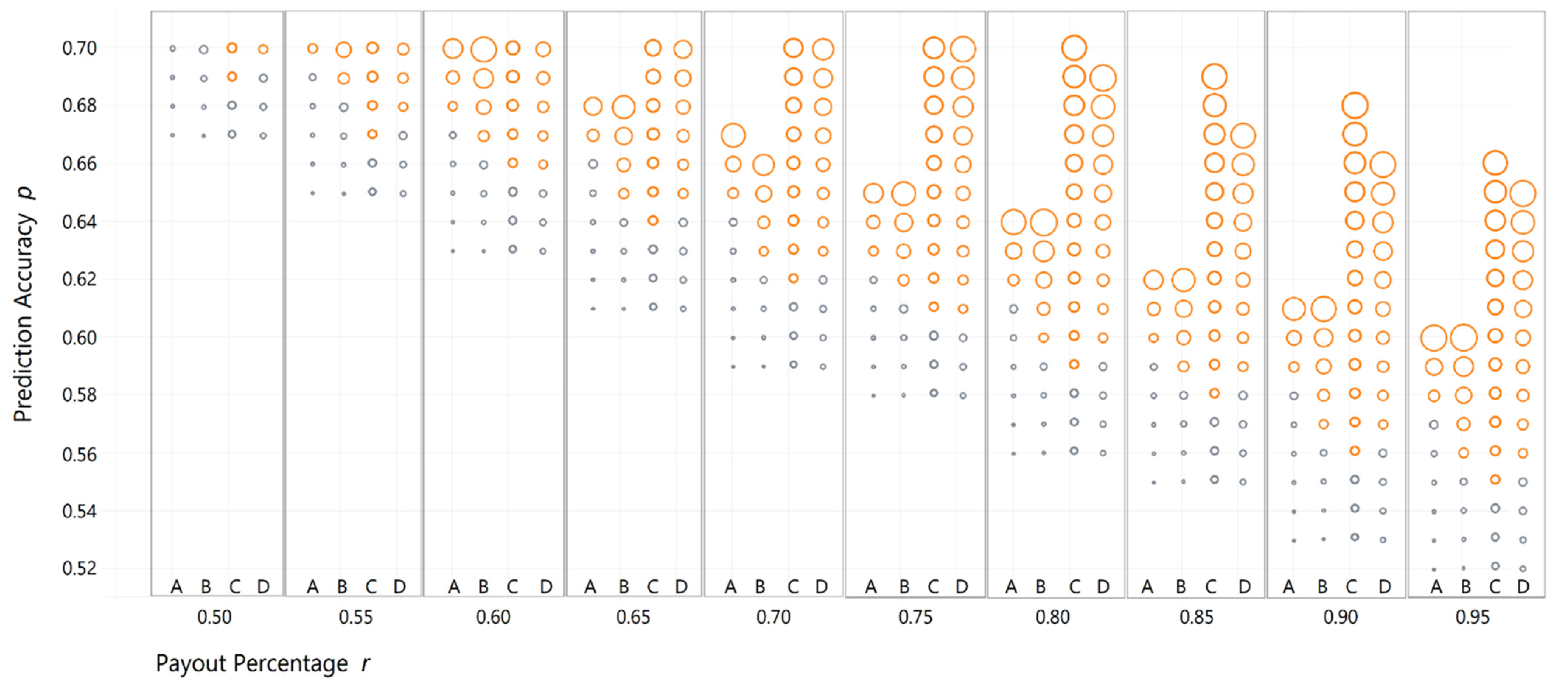
- In Figure 4, the scatter plot matrix shows the effects of prediction accuracy (y-axis) and payout percentage (x-axis) on (average of median) for each of the four strategies (columns in each box). Each circle’s (bubble’s) size linearly represents , and the color denotes whether the strategy results in (orange) or (gray);
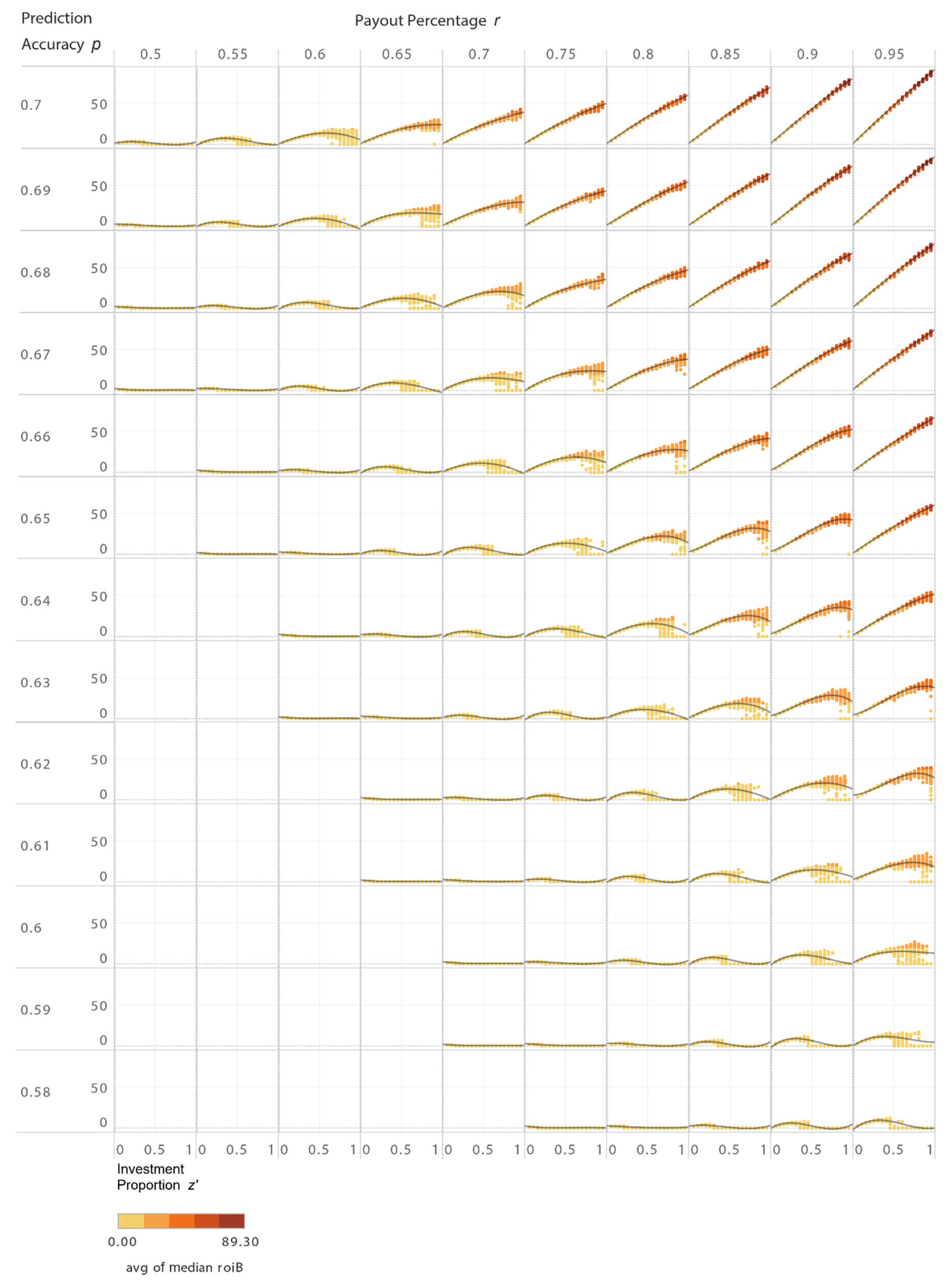
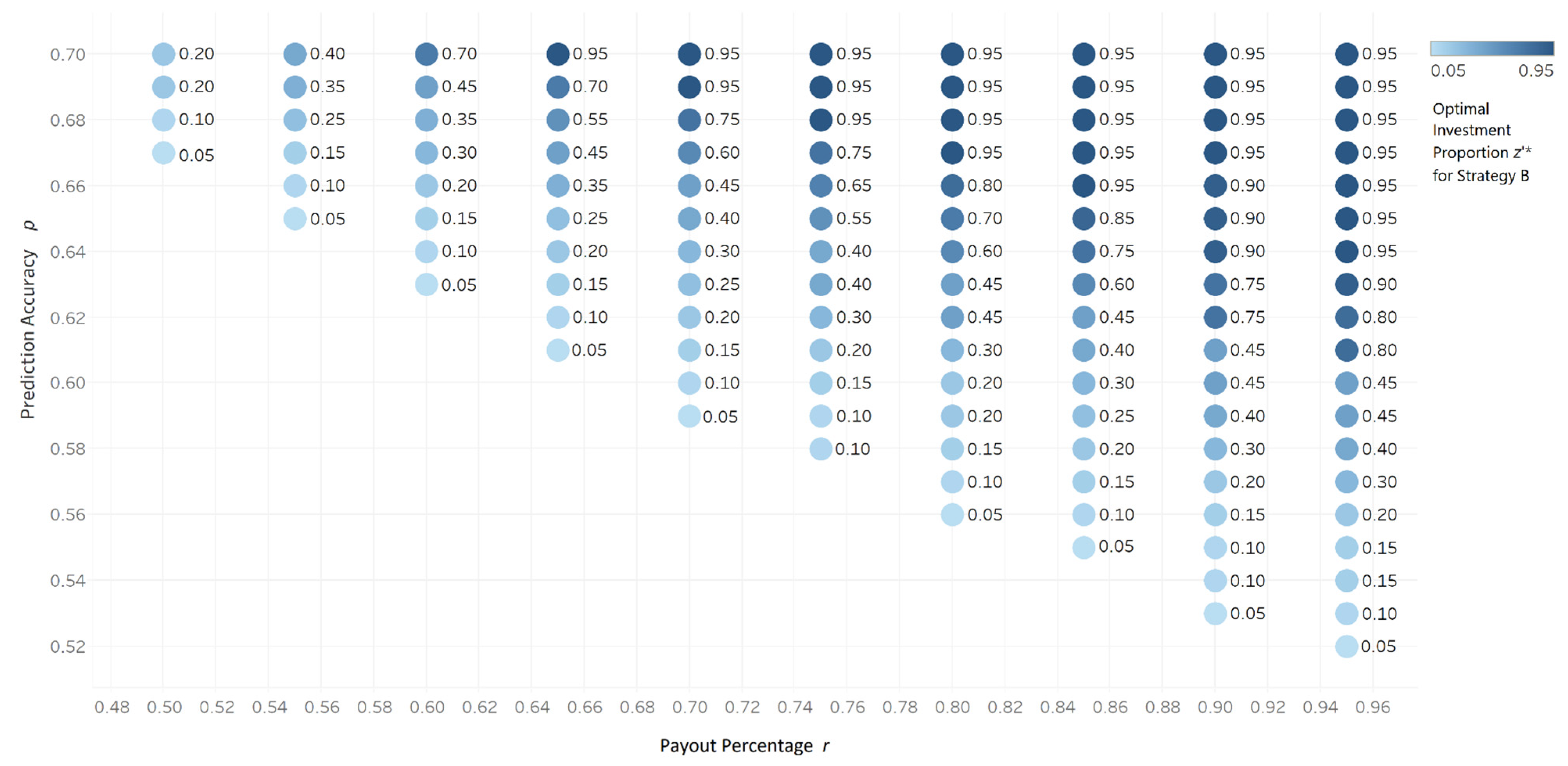
- Similarly, the scatter plot matrix in Figure 9 analyzes the impact of prediction accuracy, payout percentage, and investment proportion on (average of median) for strategy B. As a further visual clue, for strategy B is also mapped to color, and darker colors denote higher returns. To strengthen the results and insights, Figure 9 also displays best-fitted nonlinear regression curves for each plot in the matrix, where a mathematical equation is established between the factor on the x-axis and the response on the y-axis. For each pair, the equations for the curves in Figure 9 are provided in full in Supplementary File S7.
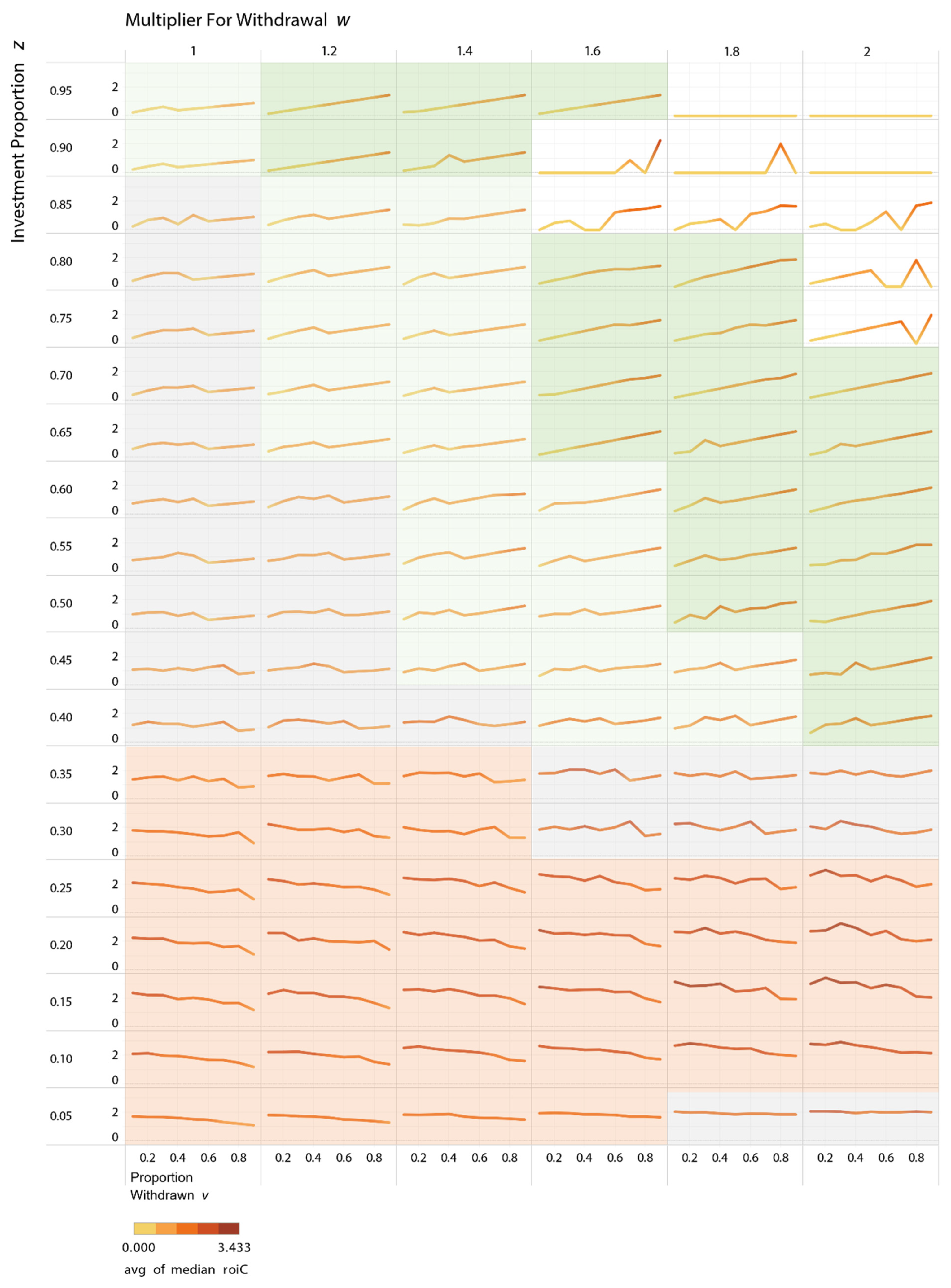
- For more than two factors, the scatter plot matrix can still be constructed by setting constant values for the additional factors. The scatter plot matrix in Figure 11 sets fixed values for prediction accuracy and payout percentage (). It also analyzes the impact of other factors—investment proportion (), on the y-axis of the matrix, the withdrawal multiplier () on the x-axis of the matrix, and the proportion withdrawn () on the x-axis of each plot—on (average of median) for strategy C. This impact is displayed on the y-axis of each plot and is denoted by color.
2.4. Regression Modeling
2.5. Modeling Binary Options
2.5.1. Metrics, Parameters, and Decision Variables
2.5.2. Assumptions
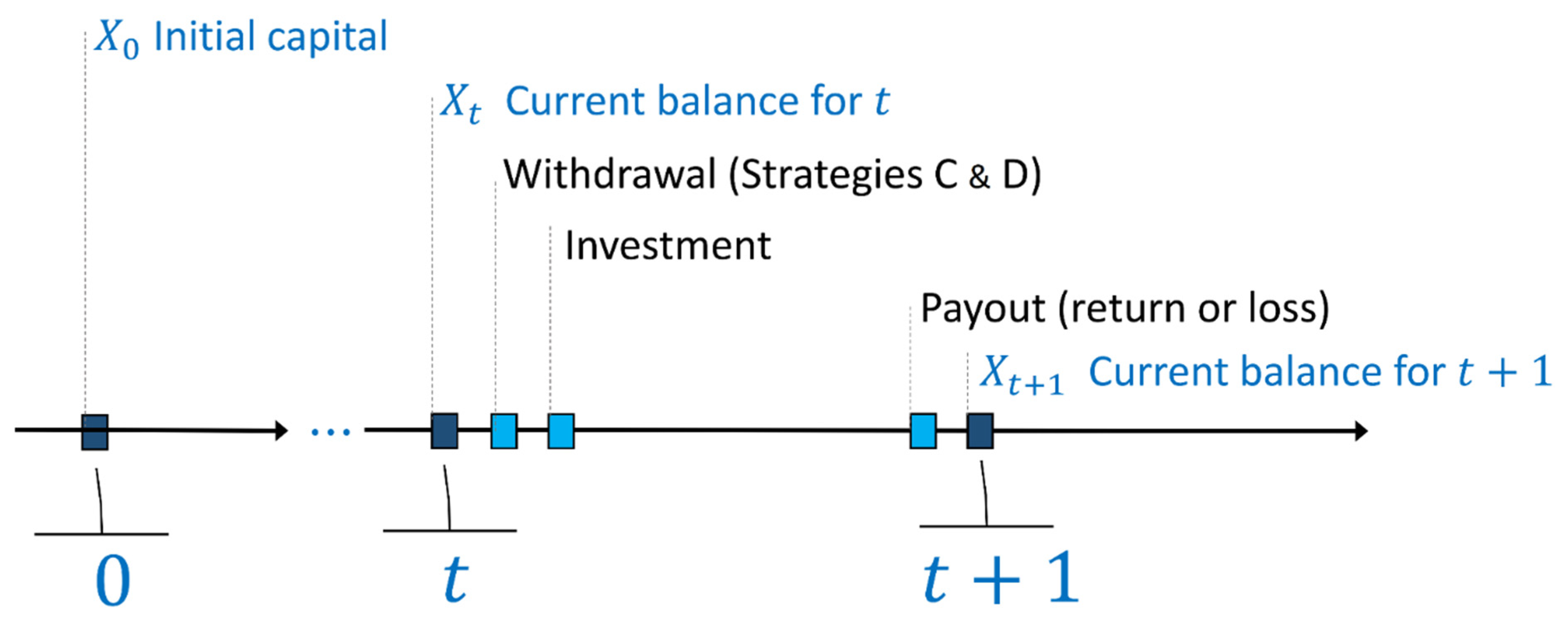
- dark blue boxes indicate the beginning of each period;
- light blue boxes indicate events during a period;
- denotes the balance at the beginning of each period: is the initial investment (), is the balance at the beginning of period , is the balance at the beginning of period , and so on;
- withdrawals (for investment strategies C and D) occur right when period begins and before any other event;
- investments for trade in each period can occur in the beginning or after any withdrawals;
- payout for each period occurs right before the end of that period and before the next period begins; and
- balance after the period payout results in the beginning balance for period .
2.5.3. Mathematical Notation
- set of periods, , where is the trading horizon.
- : initial capital available in period before the series of successive investments begins.
- : prediction accuracy, ; probability that a prediction (put or call) correctly predicts the future.
- : payout percentage, ; percentage of initial investment received if the prediction is correct.
- : trading horizon, number of periods for which successive investments are made.
- : balance available at (beginning of) period .
- : investment proportion (proportion of the current balance invested in each period) in Strategies A, C, and D, ;
- : investment proportion (proportion of the initial balance invested in each period) in Strategy B, ;
- : multiplier for withdrawal; multiplier of initial capital in deciding whether to withdraw money in Strategies C and D, ;
- : withdrawal proportion (proportion of current balance withdrawn) in Strategy C, ;
- : withdrawal proportion (proportion of surplus withdrawn) in Strategy D, .
2.5.4. Feasibility Condition
2.6. Investment Strategies
2.7. Experimental Setup and Computations
3. Results
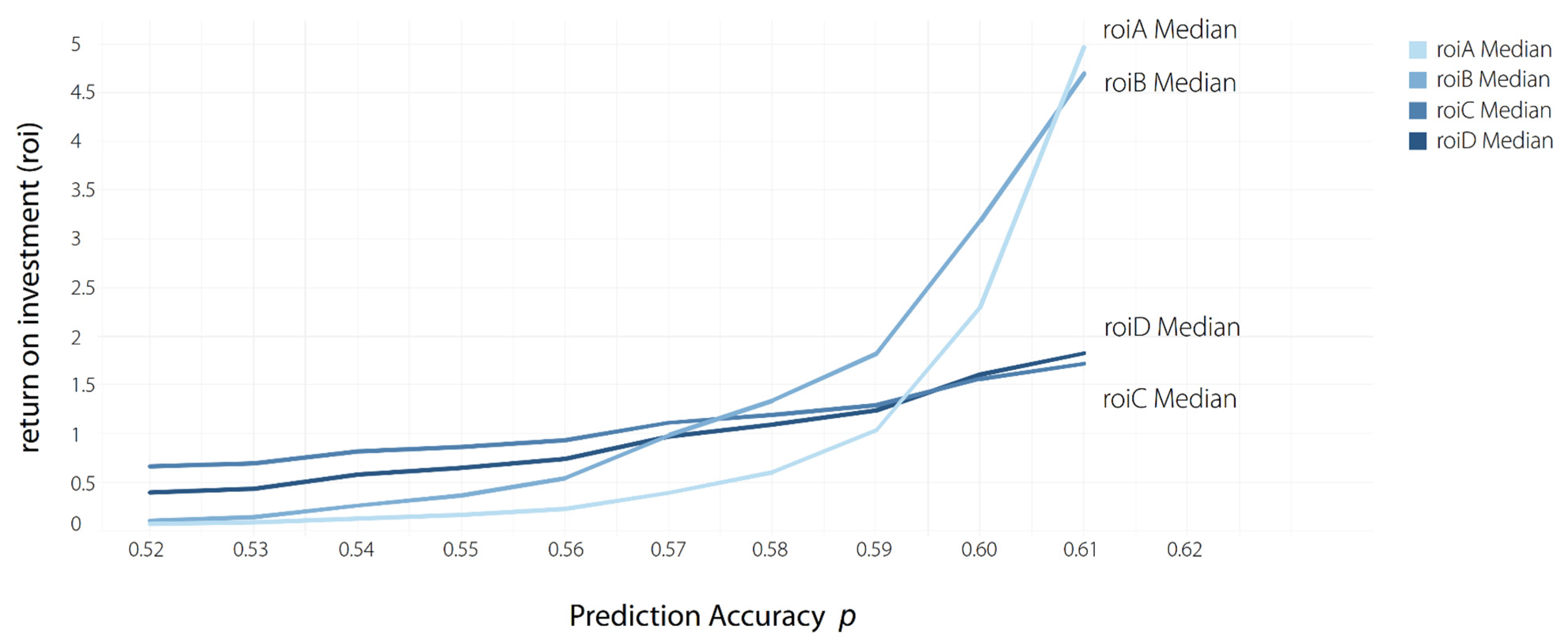
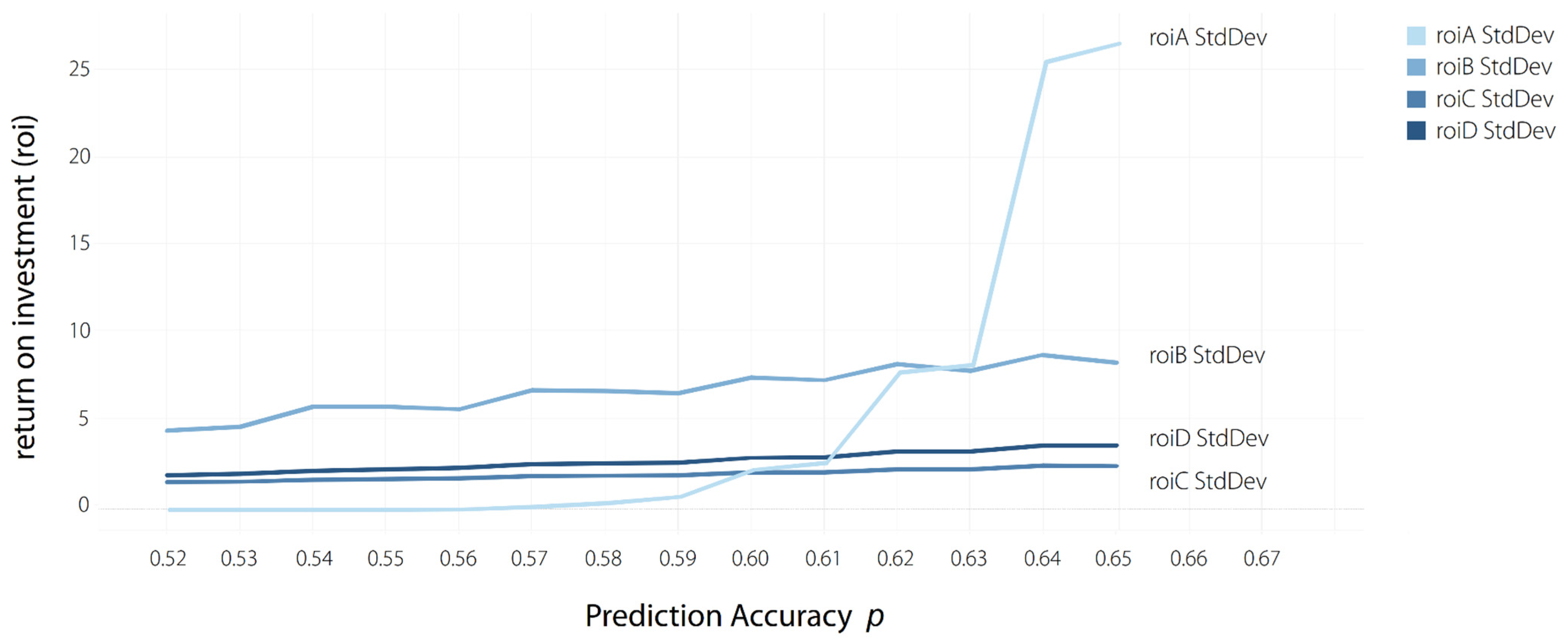
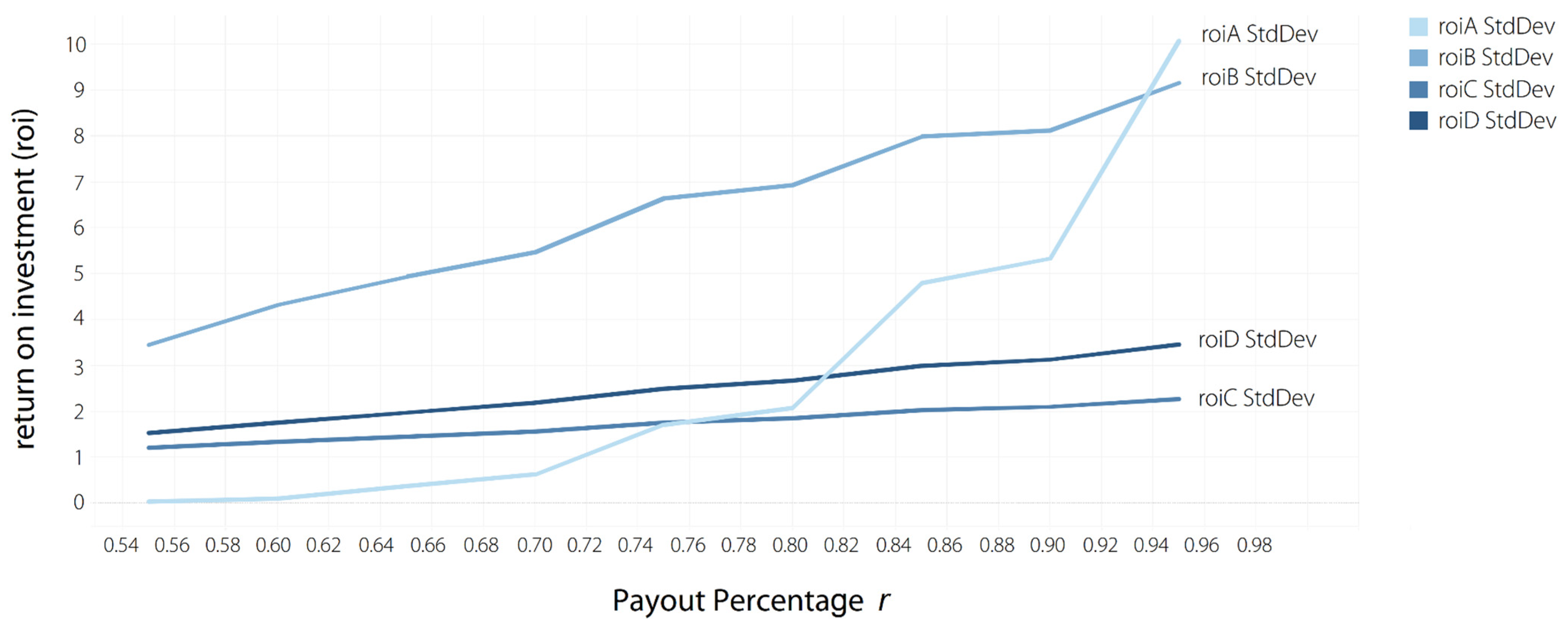
- Figure 4 analyzes the relation between the binary option parameters and across all four strategies.
- Figure 9 analyzes the relation between the binary option parameters and investment proportion in Strategy B as factors versus return on investment () as the response. For each , the figure also plots the best-fit nonlinear regression model, for which is a function of investment proportion . Supplementary File S7 of the Supplement document provides in full a nonlinear regression model and equations for the best-fit curves in Figure 9 for each pair.
- Figure 11 considers a specific binary option parameter value pair () as constant and subsequently analyzes the relation between the decision variables of Strategy C and return on investment (). A subsequent analysis was conducted for Strategy C for each pair, and the near-optimal values for the decision variables of Strategy C were computed. Supplementary File S8 provides these near-optimal values for the decision variables of Strategy C for each pair.
3.1. All Strategies
3.2. Strategy B
3.3. Strategy C
- Pink background denotes scenarios in which decreases.
- Gray background denotes scenarios in which stays mostly constant.
- Light green background denotes scenarios in which increases slightly.
- Darker green background denotes scenarios in which increases considerably, with the increasing values of the proportion withdrawn v. Meanwhile, a white background denotes scenarios in which no consistent patterns exist.
- The following observations are made from Figure 11.
- Pink plots: Not making any withdrawals at all () is typically more profitable (higher ) when the investment proportion has low values, less than ;
- Gray plots: For certain value ranges, is insensitive to changes in ;
- Green plots: The return typically increases as the values of the proportion withdrawn increase when the investment proportion is , and the multiplier for withdrawal is . In other words, higher values of are preferred for higher with higher values of and
4. Conclusions
4.1. Research Scope
4.2. Findings
4.3. Future Work
Supplementary Materials
Author Contributions
Funding
Data Availability Statement
Acknowledgments
Conflicts of Interest
References
- Page, L.; Siemroth, C. How Much Information Is Incorporated into Financial Asset Prices? Experimental Evidence. Rev. Financ. Stud. 2020, 34, 4412–4449. [Google Scholar] [CrossRef]
- Cofnas, A.; Wiggin, A. Trading Binary Options: Strategies and Tactics; John Wiley & Sons, Incorporated: Hoboken, NJ, USA, 2016. [Google Scholar]
- Harmon, G. Trading Options: Using Technical Analysis to Design Winning Trades; Wiley: Hoboken, NJ, USA, 2014. [Google Scholar]
- Raw, H. Binary Options: Fixed Odds Financial Bets; Harriman House Limited: Petersfield, UK, 2011. [Google Scholar]
- Šitavanc, J. Exotic Options and Their Feasible Usage as Investment Instrument. Master’s Thesis, Brno University of Technology, Brno, Czech Republic, 2010. [Google Scholar]
- Cboe. Available online: http://www.cboe.com/institutional/pdf/listedbinaryoptions.pdf (accessed on 26 March 2021).
- Martinkute-Kauliene, R. Exotic Options: A Chooser Option and Its Pricing. Business. Manag. Educ. 2012, 10, 289–301. [Google Scholar] [CrossRef]
- Muravyev, D.; Pearson, N.D. Options Trading Costs Are Lower than You Think. Rev. Financ. Stud. 2020, 33, 4973–5014. [Google Scholar] [CrossRef]
- Gogol, E.; Glinberg, D.; Michaels, D. Processing Binary Options in Future Exchange Clearing. U.S. Patent No. 8,224,742, 2012. [Google Scholar]
- Jaycobs, R.; Glantz, N.; Les Walker, J. Systems and Methods for Computing an Index for a Binary Options Transaction. U.S. Patent US20120221456A1, 2019. [Google Scholar]
- Genzer, Y.; Avraham, G. Binary Options Trading System. U.S. Patent No. 2017/0076370, 7 July 2017. [Google Scholar]
- Montanaro, D.A.; Bickford, M.T.; Burns, J.P.; Masciale, C.P.; Ebner, S.R. Binary Options on an Organized Exchange and the Systems and Methods for Trading the Same. U.S. Patent No. 8,738,499, 27 May 2014. [Google Scholar]
- Mitsuhiro, M.; Ota, Y. Recovery of Foreign Interest Rates from Exchange Binary Options. Comput. Technol. Appl. 2015, 190, 76–88. [Google Scholar] [CrossRef][Green Version]
- Jaycobs, R.; Bradshaw, T.D.; Poulos, J. Binary Options on Selected Indices. U.S. Patent No. 2017/0053350, 8 October 2017. [Google Scholar]
- Bigiotti, A.; Navarra, A. Optimizing Automated Trading Systems. In Advances in Intelligent Systems & Computing 2019; The 2018 International Conference on Digital Science; Springer: Cham, Switzerland, 2018; pp. 254–261. [Google Scholar] [CrossRef]
- Rumpa, L.D.; Limbongan, M.E.; Biringkanae, A.; Tammu, R.G. Binary Options Trading: Candlestick Prediction Using Support Vector Machine (SVM) on M5 Time Period. In Proceedings of the IOP Conference Series. Materials Science and Engineering, Annual Conference on Computer Science and Engineering Technology (AC2SET), Medan, Indonesia, 23 September 2020; IOP Publishing: Bristol, UK, 2021; Volume 1088, p. 012107. [Google Scholar] [CrossRef]
- Theodorou, T.-I.; Zamichos, A.; Skoumperdis, M.; Kougioumtzidou, A.; Tsolaki, K.; Papadopoulos, D.; Patsios, T.; Papanikolaou, G.; Konstantinidis, A.; Drosou, A.; et al. An AI-Enabled Stock Prediction Platform Combining News and Social Sensing with Financial Statements. Future Internet 2021, 13, 138. [Google Scholar] [CrossRef]
- Guojun, Y.; Qingxian, X. A New Numerical Method for Pricing Binary Options in the CEV Process. In Proceedings of the International Conference on E-Business and E-Government (ICEE), Shanghai, China, 6–8 May 2011; IEEE Publications: Piscataway, NJ, USA, 6–8 May; pp. 1–4. [Google Scholar]
- Kim, H.-J.; Moon, K.-S. Variable Time-Stepping Hybrid Finite Difference Methods for Pricing Binary Options. Bull. Korean Math. Soc. 2011, 48, 413–426. [Google Scholar] [CrossRef][Green Version]
- Guo-jun, Y. Study on the Pricing of Binary Options in the CEV Process Based on Semidiscretization. J. Syst. Eng. 2012. Available online: https://en.cnki.com.cn/Article_en/CJFDTotal-XTGC201201005.htm (accessed on 26 March 2021).
- Thavaneswaran, A.; Appadoo, S.S.; Frank, J. Binary Option Pricing Using Fuzzy Numbers. Appl. Math. Lett. 2013, 26, 65–72. [Google Scholar] [CrossRef]
- Miyake, M.; Inoue, H.; Shi, J.; Shimokawa, T. A Binary Option Pricing Based on Fuzziness. Int. J. Inf. Technol. Decis. Mak. 2014, 13, 1211–1227. [Google Scholar] [CrossRef]
- Hyong-Chol, O.; Dong-Hyok, K.; Jong-Jun, J.; Song-Hun, R. Integrals of Higher Binary Options and Defaultable Bonds with Discrete Default Information. Electron. J. Math. Anal. Appl. 2014, 2, 190–214. [Google Scholar]
- Yuan, G. Pricing Binary Options Based on Fuzzy Number Theory. Rev. Tec. De La Fac. De Ing. Univ. Del Zulia 2016, 39, 384–391. [Google Scholar]
- Dastranj, E.; Latifi, R. Pricing of Binary Options in Financial Markets with Stochastic Analysis. J. Econ. Manag. Perspect. 2017, 11, 704–709. [Google Scholar]
- Gao, M. Early Exercise Options with Discontinuous Payoff. Ph.D. Thesis, The University of Manchester, Manchester, UK, 2017. [Google Scholar]
- Grande, J.S.-L.; Febrián, A.S.-R. A Quantum Mechanics Approach to Pricing Binary Options: An Application to the S&P, 500. 2018. Available online: https://repositorio.comillas.edu/xmlui/handle/11531/26212 (accessed on 26 March 2021).
- Ferrando, S.; Catuogno, P.; Gonzalez, A. Efficient Hedging Using a Dynamic Portfolio of Binary Options. 2009. Available online: https://math.ryerson.ca/~ferrando/publications/effBinHedg.pdf (accessed on 26 March 2021).
- Tsai, W.C. Improved Method for Static Replication under the CEV Model. Financ. Res. Lett. 2014, 11, 194–202. [Google Scholar] [CrossRef]
- Acharya, D. Spanning with Binary Options: A Vector Lattice Approach. Master’s Thesis, Ryerson University, Toronto, ON, Canada, 2019. [Google Scholar]
- Mercurio, P.J.; Wu, Y.; Xie, H. Portfolio Optimization for Binary Options Based on Relative Entropy. Entropy 2020, 22, 752. [Google Scholar] [CrossRef] [PubMed]
- Pan, W.; Li, J.; Li, X. Portfolio Learning Based on Deep Learning. Future Internet 2020, 12, 202. [Google Scholar] [CrossRef]
- Pietrzyk, R.; Rokita, P. Determination of the Own Funds Requirements for the Risk of Binary Options. In Springer Proceedings in Business & Economics; Springer: Berlin/Heidelberg, Germany, 2018; pp. 23–32. [Google Scholar] [CrossRef]
- Oleas, M.E.E.; Palacios, M.E.A. Strategy to Prevent the Risk of Trading in Binary Options. China–USA Bus. Rev. 2019, 18, 33. [Google Scholar] [CrossRef]
- Jaycobs, R.; Glantz, N.; Les Walker, J. Systems and Methods of Detecting Manipulations on a Binary Options Exchange. U.S. Patent US10304130B2, 27 May 2019. [Google Scholar]
- Barnes, P. The Use of Contracts for Difference (‘CFD’) Spread Bets and Binary Options (‘Forbin’) to Trade Foreign Exchange (‘Forex’) Commodities, and Stocks and Shares in Volatile Financial Markets. 2021, Retrieved from MPRA Paper 105743. Available online: https://mpra.ub.uni-muenchen.de/105743/. (accessed on 22 May 2022).
- Bégin, J.-F.; Dorion, C.; Geneviève, G. Idiosyncratic Jump Risk Matters: Evidence from Equity Returns and Options. Rev. Financ. Stud. 2020, 33, 155–211. [Google Scholar] [CrossRef]
- Pandey, P.; Snekkenes, E. Using Financial Instruments to Transfer the Information Security Risks. Future Internet 2016, 8, 20. [Google Scholar] [CrossRef]
- Novruzova, O.B.; Pronina, Y.O.; Vorobeva, E.S. Binary Options as New Financial Instruments and Their Integration into the Financial Sector. In 2nd International Scientific and Practical Conference “Modern Management Trends and the Digital Economy: From Regional Development to Global Economic Growth”; Atlantis Press: Dordrecht, The Netherlands, 2020; pp. 760–763. [Google Scholar]
- Glasserman, P. Monte Carlo Methods in Financial Engineering; Springer Science & Business Media: New York, NY, USA, 2013; Volume 53. [Google Scholar]
- Duran, A.; Bommarito, M.J. A Profitable Trading and Risk Management Strategy despite Transaction Costs. Quant. Financ. 2011, 11, 829–848. [Google Scholar] [CrossRef]
- Leal, S.J.; Napoletano, M.; Roventini, A.; Fagiolo, G. Rock around the Clock: An Agent-Based Model of Low-And High-Frequency Trading. J. Evol. Econ. 2016, 26, 49–76. [Google Scholar] [CrossRef]
- Cong, F.; Oosterlee, C.W. Multi-Period Mean-Variance Portfolio Optimization Based on Monte-Carlo Simulation. J. Econ. Dyn. Control 2016, 64, 23–38. [Google Scholar] [CrossRef]
- Suzuki, K. Optimal Pair-Trading Strategy Over Long/Short/Square Positions—Empirical Study. Quant. Financ. 2018, 18, 97–119. [Google Scholar] [CrossRef]
- Nouri, K.; Abbasi, B.F.; Omidi, L.; Torkzadeh. Digital Barrier Options Pricing: An Improved Monte Carlo Algorithm. Math. Sci. 2016, 10, 65–70. [Google Scholar] [CrossRef]
- Holcomb, Z.C. Fundamentals of Descriptive Statistics; Routledge: New York, NY, USA, 1997; ISBN 9781884585050. [Google Scholar]
- Kim, H.Y. Statistical Notes for Clinical Researchers: Assessing Normal Distribution (2) Using Skewness and Kurtosis. Restor. Dent. Endod. 2013, 38, 52–54. [Google Scholar] [CrossRef]
- NIST/SEMATECH e-Handbook of Statistical Methods; (NIST Handbook 151); National Institute of Standards and Technology: Gaithersburg, MD, USA, 2012. Available online: https://www.itl.nist.gov/div898/handbook/ (accessed on 1 July 2022).
- Ertek, G.; Tokdemir, G.; Sevinç, M.; Tunç, M.M. New knowledge in strategic management through visually mining semantic networks. Inf. Syst. Front. 2017, 19, 165–185. [Google Scholar] [CrossRef][Green Version]
- Keim, D.A. Information Visualization and Visual Data Mining. IEEE Trans. Vis. Comput. Graph. 2002, 8, 1–8. [Google Scholar] [CrossRef]
- Riazoshams, H.; Midi, H.; Ghilagaber, G. Robust Nonlinear Regression: With Applications Using, R; John Wiley & Sons: Hoboken, NJ, USA, 2019; ISBN 9781118738061. [Google Scholar]
- Kaggle. State of Machine Learning and Data Science 2021; 2021, p. 33. Available online: https://www.kaggle.com/kaggle-survey-2021. (accessed on 27 June 2022).
- Thachuk, R. Binary Options-the Next Big Retail Investing Boom? FOW Magazine, May 2010. Available online: https://www.botlc.or.th/item/article/02000045931 (accessed on 22 May 2022).
- Rosa, L. A Profitable Hybrid Strategy for Binary Options. 2016. Available online: http://www.advancedsourcecode.com/binaryoptions.pdf (accessed on 26 March 2021).
- Dichtl, H.; Drobetz, W. Dollar-Cost Averaging and Prospect Theory Investors: An Explanation for a Popular Investment Strategy. J. Behav. Financ. 2011, 12, 41–52. [Google Scholar] [CrossRef]
- Vezeris, D.; Kyrgos, T.; Schinas, C. Take Profit and Stop Loss Trading Strategies Comparison in Combination with an MACD Trading System. J. Risk Financ. Manag. 2018, 11, 56. [Google Scholar] [CrossRef]
- Khorikov, V. Unit Testing Principles, Practices, and Patterns, 1st ed.; Manning Publications: New York, NY, USA, 2020. [Google Scholar]
- Fu, M.C. Handbook of Simulation Optimization, International Series in Operations Research & Management Science; Springer: New York, NY, USA, 2015. [Google Scholar]
- Giunta, G.; Benedetto, F. Empirical Case Study of Binary Options Trading: An Interdisciplinary Application of Telecommunications Methodology to Financial Economics. Int. J. Interdiscip. Telecommun. Netw. 2012, 4, 54–63. [Google Scholar] [CrossRef]
- Benedetto, F.; Giunta, G. Communication Services Applied to Business: A Simple Algorithm for Personal Trading. In Proceedings of the 2013 IEEE 24th Annual International Symposium on Personal, Indoor and Mobile Radio Communications (PIMRC), London, UK, 8–11 September 2013. [Google Scholar]
- Brits, F.S. Utilising Technical Analysis to Generate Buy-and-Sell Signals to Trade Binary Options. Ph.D. Thesis, North-West University, Potchefstroom Campus, Pochefstroom, South Africa, 2016. Available online: https://dspace.nwu.ac.za/bitstream/handle/10394/24998/Brits_FS_2016.pdf?sequence=1&isAllowed=y (accessed on 22 May 2022).
- Basdekidou, V.A. Nonfarm employment report trading with binary options & temporal functionalities. Ann. Univ. Apulensis Ser. Oeconomica 2017, 19, 15–24. [Google Scholar]
- Kolková, A.; Lenertová, L. Binary Options as a Modern Fenomenon of Financial Business. Int. J. Entrep. Knowl. 2016, 4, 52–59. [Google Scholar] [CrossRef][Green Version]
- Hui, C.H. One-Touch Double Barrier Binary Option Values. Appl. Financ. Econ. 1996, 6, 343–346. [Google Scholar] [CrossRef]
- Smith, K. American Binary FX Options: From Theoretical Value to Market Price. Ph.D. Thesis, University of Western Australia, Perth, Australia, 2010. Available online: https://api.research-repository.uwa.edu.au/ws/portalfiles/portal/3215595/Smith_Kurt_2010.pdf (accessed on 22 May 2022).
- Hyong-Chol, O.; Kim, M.-C. Higher Order Binary Options and Multiple Expiry Exotics. Electronic. J. Math. Anal. Appl. 2013, 1, 247–259. [Google Scholar]
- Chiang, M.-H.; Fu, H.-H.; Huang, Y.-T.; Lo, C.-L.; Shih, P.-T. Analytical Approximations for American Options: The Binary Power Option Approach. J. Financ. Stud. 2018, 26, 91. [Google Scholar]
- Gao, M.; Wei, Z. The Barrier Binary Options. J. Math. Financ. 2020, 10, 140–156. [Google Scholar] [CrossRef][Green Version]
- SEC. Investor Alert: Binary Options and Fraud. 2016. Available online: https://www.sec.gov/investor/alerts/ia_binary.pdf. (accessed on 26 March 2021).
- All-Too-Often Fraudulent. 2019. Available online: https://www.finra.org/investors/alerts/binary-options (accessed on 26 March 2021).
- FCA: Binary Options. 2020. Available online: https://www.fca.org.uk/consumers/binary-options. (accessed on 26 March 2021).
- FSMA: FSMA Regulation Governing the Distribution of Certain Derivative Financial Instruments (Binary Options, Cfds, Etc.). Available online: https://www.fsma.be/en/faq/fsma-regulation-governing-distribution-certain-derivative-financial-instruments-binary-options-0 (accessed on 26 March 2021).
- O’Kane, J. Regulators Ban Short-Term Binary Options but Warn of Enforcement Challenges. 2017. Available online: https://www.theglobeandmail.com/report-on-business/canadian-regulators-ban-short-term-binary-options-the-leading-type-of-investment-fraud/article36419085/ (accessed on 26 March 2021).
- AFM: Dutch Regulator Proposes Ban on Advertising of Binary Options. 2017. Available online: https://financefeeds.com/dutch-regulator-proposes-ban-advertising-binary-options/ (accessed on 26 March 2021).
- ESMA: European Securities and Markets Authority Decision (EU) 2018/795 of 22 May 2018. Available online: https://eur-lex.europa.eu/legal-content/EN/TXT/HTML/?uri=CELEX:32018X0601(01)&qid=1528704280041&from=en (accessed on 26 March 2021).
- ESMA: ESMA Ceases Renewal of Product Intervention Measure Relating to Binary Options. 2019. Available online: https://www.esma.europa.eu/press-news/esma-news/esma-ceases-renewal-product-intervention-measure-relating-binary-options. (accessed on 26 March 2021).
- AFM. AFM Takes National Measures to Prohibit Binary Options and to Restrict the Marketing or Sales of CFDs. 17 April. Available online: https://www.afm.nl/en/consumenten/nieuws/2019/apr/binaire-opties-cfds-interventies (accessed on 26 March 2021).
- Fantato, D. FCA Warns Investors Against Binary Options. 2017. Available online: https://www.ftadviser.com/investments/2017/11/15/fca-warns-investors-against-binary-options/ (accessed on 26 March 2021).
- Pape, G. Don’t Gamble on Binary Options. 2010. Available online: https://www.forbes.com/sites/investor/2010/07/27/dont-gamble-on-binary-options/. (accessed on 26 March 2021).
- Micallef, R. The legal and regulatory aspects of online binary options under Maltese law. Master’s Thesis, University of Malta, Msida, Malta, 2016. Available online: https://www.um.edu.mt/library/oar/handle/123456789/17513 (accessed on 26 May 2021).
- Nekritin, A. Binary Options: Strategies for Directional and Volatility Trading; Wiley Trading Series; John Wiley & Sons: Hoboken, NJ, USA, 2012; Available online: https://www.wiley.com/en-us/Binary+Options:+Strategies+for+Directional+and+Volatility+Trading-p-9781118528693 (accessed on 26 May 2021).


| Symbol | Name | Parameter or Decision | Min Value | Max Value | Increment | Number of Values |
|---|---|---|---|---|---|---|
| Prediction Accuracy | Parameter | 0.50 | 0.70 | 0.01 | 21 | |
| Payout Percentage | Parameter | 0.50 | 0.95 | 0.05 | 10 | |
| Investment Proportion | Decision | 0.05 | 0.95 | 0.05 | 19 | |
| Multiplier For Withdrawal | Decision | 1.00 | 2.00 | 0.20 | 6 | |
| Withdrawal Proportion | Decision | 0.10 | 0.90 | 0.10 | 9 |
Publisher’s Note: MDPI stays neutral with regard to jurisdictional claims in published maps and institutional affiliations. |
© 2022 by the authors. Licensee MDPI, Basel, Switzerland. This article is an open access article distributed under the terms and conditions of the Creative Commons Attribution (CC BY) license (https://creativecommons.org/licenses/by/4.0/).
Share and Cite
Ertek, G.; Al-Kaabi, A.; Maghyereh, A.I. Analytical Modeling and Empirical Analysis of Binary Options Strategies. Future Internet 2022, 14, 208. https://doi.org/10.3390/fi14070208
Ertek G, Al-Kaabi A, Maghyereh AI. Analytical Modeling and Empirical Analysis of Binary Options Strategies. Future Internet. 2022; 14(7):208. https://doi.org/10.3390/fi14070208
Chicago/Turabian StyleErtek, Gurdal, Aysha Al-Kaabi, and Aktham Issa Maghyereh. 2022. "Analytical Modeling and Empirical Analysis of Binary Options Strategies" Future Internet 14, no. 7: 208. https://doi.org/10.3390/fi14070208
APA StyleErtek, G., Al-Kaabi, A., & Maghyereh, A. I. (2022). Analytical Modeling and Empirical Analysis of Binary Options Strategies. Future Internet, 14(7), 208. https://doi.org/10.3390/fi14070208