A Framework to Model Bursty Electronic Data Interchange Messages for Queueing Systems ^†

Abstract

Within a supply chain organisation, where millions of messages are processed, reliability and performance of message throughput are important. Problems can occur with the ingestion of messages; if they arrive more quickly than they can be processed, they can cause queue congestion. This paper models data interchange (EDI) messages. We sought to understand how best DevOps should model these messages for performance testing and how best to apply smart EDI content awareness that enhance the realms of Ambient Intelligence (Aml) with a Business-to business (B2B) supply chain organisation. We considered key performance indicators (KPI) for over- or under-utilisation of these queueing systems. We modelled message service and inter-arrival times, partitioned data along various axes to facilitate statistical modelling and used continuous parametric and non-parametric techniques. Our results include the best fit for parametric and non-parametric techniques. We noted that a one-size-fits-all model is inappropriate for this heavy-tailed enterprise dataset. Our results showed that parametric distribution models were suitable for modelling the distribution’s tail, whilst non-parametric kernel density estimation models were better suited for modelling the head of a distribution. Depending on how we partitioned our data along the axes, our data suffer from quantisation noise.

1. Introduction

As new businesses emerge and existing businesses expand, there is a heavy reliance on the need to keep costs low and maximise profits. Queueing systems play a fundamental role that helps businesses within the supply chain domain reduce cost by supporting high availability, resilient connectivity and operational efficiency. Further costs can be achieved by adopting smartness to these existing queueing applications and Supply Chain environments that will advance the Intelligence Age of these systems [1].

When demand exceeds supply, queueing systems provide a more streamlined experience by preventing job loss and supporting queue and job prioritisation. However, like all computing systems, queues are not immune to performance and reliability problems, including latency, bottlenecks, scalability, and the challenges faced with the unpredictable arrival of incoming messages [2]. Real-word queueing systems also have challenges not encountered by abstract models, such as re-processing failed jobs and malformed messages.

Queueing systems can support the effective passing of business-to-business (B2B) transactions through a supply chain network. With the demand for digital having gone global, there is an increased need for digitised environments that can support these B2B transactions alongside their associated paperless contracts and traceability of goods.

Millions of B2B messages can be ingested by a queueing application. When modelling these messages, it is imperative that we can capture the real-time aspects, including the temporal ordering of message arrivals, which was first studied by Lampart [3]. Rounding or truncating an event’s timestamp at the time of writing to a systems log file or software application can obfuscate the exact ordering of events, cause quantisation noise and lead to challenges fitting particular distributions [4].

Stress testing queueing systems is crucial to uncovering functional and performance problems in large-scale systems. The messages order, volume, pace, and dependencies are critical for distribution modelling. Understanding these features is important before applying queueing models, such as the GI/GI/1 model, which assumes message independence of the inter-arrival and service times [5]. If messages are dependent whereby the service times are dependent on the messages’ inter-arrival times, then a G/G/1, in its most general sense, might be more appropriate.

For any queueing system, different products are always looking for ways to make product improvements. IBM has developed “Uniform Clusters”. It can automatically create connection channels and support horizontal scaling across multiple matching queues [6]. It does, however, have some limitations. Load balancing problems may occur if there are more queue managers than applications [7].

Another application that IBM has developed for MQ is “Streaming Queues,” which allows copying every message to a second queue. If the customer wants a carbon copy of their data for later retrieval, it can be used [8].

In Apache Kafka, a broker may be alive but unable to establish a new connection due to a failed DNS resolution which may be hard to detect. In the latest 3.1 release, new functionality has been implemented to help identify this type of problem by including KIP-748 [9].

“Pre-staging messages at a remote location” is an innovative patent that, if applied, supports remotely storing a vast number of messages in a data storage system that will form a message queue. Many queue managers can then access these messages [10].

1.1. Background and Previous Work

This paper extends the results from our conference paper [11]. In this subsection, we give the background on queueing systems used for EDI-type messages, and review some related literature.

1.1.1. Performance of Message Queueing Systems

LinkedIn wanted to move away from batch-oriented systems towards real-time publish–subscribe systems. Their requirement was a system capable of processing 10 billion messages per day, with demand peaking at 172,000 messages per second. Initially, they considered ActiveMQ, but decided to develop Kafka [12], which was subsequently made open source.

The performance of Kafka was studied, and the impact of tuning specific parameters was considered [13]. The study found that performance was variable, depending on both system infrastructure and messages processed. A correlation between packet sizes and sending intervals was also observed.

The performance of the IBM MQ JMS Server was also undertaken [14]. This study considered the study of the capacity of the system, considering filters, message sizes and number of publishers, subscribers and topics. Message size influenced server performance, in terms of both message and data throughput. Likewise, message replication grade and the number of filters used also influenced server capacity. On the other hand, the number of topics had limited impact on capacity.

1.1.2. EDI Messaging

EDI consists of five critical components:

• Message specification;
• Syntax and format;
• Partner agreements;
• Timing;
• Addressing.

We make use of some subsidiary components under the message specification, syntax and format components, including a message’s file size, source file size, bytes, maps, etc., from the attached XML documents. We also take into account a message’s action and category. We use these as a novel approach to identify bursty and non-bursty messages. We also use these to partition the dataset to facilitate modelling of our queueing system.

1.1.3. EDI Deployments

When looking at a supply chain organisation, we pay particular attention to B2B messages, also known as EDI messages. We note that EDI messages electronically support the trading of transactions between a customer and its trading partner. EDI messaging allows customers and trading partners to trade electronically using digital signatures. Some of the beneficial features of EDI include message integrity, confidentiality, interoperability, non-repudiation of a contract and traceability of a transaction [15]. Deploying EDI in B2B organisations can save up to 15 min per invoice transaction query between a supplier and its trading partner [16]. EDI was born in the UK, and its expected growth in 1991 was perceived to grow at a sigmoidal rate [17]. EDI is deployed in many organisations, with some examples shown in

Table 1. Industries using EDI.

Standard	Industry
ANA	Food, Retail, distribution
TF2	Health Service
FLEETNET	Fleet Car Industry
EDISHIP	Shipping/Forwarding
PHARMEDI	Pharmaceutical
EDICON	Construction
EDICUG	Components
BEDIS	Book Publishing Libraries
PIPE	Paper/Printing
EDIA	Banking, Transport
ODETTE	Automotive

[17].

Our research focuses on modelling EDI messages through queueing systems. EDI messages are bursty. One incoming message may result in many messages being sent to a queue at once. These bursty messages may cause bottlenecks in a queueing system, and so understanding them is useful for stress testing and simulating queue environments. When modelling these messages, it is important to identify what characteristics determine whether an EDI message will be bursty. For example, when a customer sends in 100 transactions, are you stress testing a queueing system for 100 individual transactions or a burst of those transactions? The system may need to be ready for a single transaction resulting in hundreds of messages ingested by a queue.

We found that the Department of Defence developed and advanced system architecture to support EDI messages based on different modelling and simulation techniques. This was motivated by ever-growing transaction sizes and the inter-twining of many applications. They used modelling and simulation techniques to support the decision making of their advanced system architecture [15].

EDI implementations have also been studied. For example, one study investigated if the adoption of EDI improves customer service [18]. The main factors that influence a companies decision to implement EDI were also considered [19]. Their findings indicate that companies will adopt EDI depending on whether their business partners are doing so. A study of EDI and the motor trade industry aimed to partly examine the extent to which EDI was used in the motor carrier industry and potential problems that might hinder the use of EDI for these motor carriers [20].

We note that although EDI has been researched in different areas, none of these studies addresses EDI implementation regarding simulation and performance testing, specifically around queueing systems and modelling service and inter-arrival times. We note that these EDI messages suffer from burstiness. We found little evidence of research around the field of being able to identify using different elements of an EDI message of a bursty versus a non-bursty message. We believe this is a gap in the research that should be addressed.

1.1.4. Industry 4.0

Intelligent advances within the IT domain can benefit a Supply Chain network. Industry 4.0 is driven by IT advances like smart factories using smart technologies [21]. In the field of B2B transactions, the concept of Industry 4.0 plays a vital role in the automatic exchange of information between different business entities. Offering full traceability and transparency between suppliers, manufacturers, and customers is essential for streamlined autonomous services within a Supply Chain. The Supply Chain Industry plays a pivotal role in the transportation and traceability of goods. Adopting Industry 4.0 can have many additional benefits, like a 53% chance of order fulfilment opportunities and a 71% of opportunities in procurement [22]. Other benefits include the flexibility and scalability of Supply Chain operating models that extend upon Supply Chain productivity [23]. Operational Research algorithm’s using the Supply Chain Information System via the cloud can address problems relating to the routing of transport and the scheduling of deliveries within cities [24]. A lack of standards around IT security can sway a company from adopting the 4.0 concept. A taxonomy of advantages and disadvantages of Industry 4.0 and the Supply Chain network has been researched [25]. Frameworks have been developed to help companies assess if they are ready to adopt Industry 4.0 supply chains [26].

1.1.5. AmI, IoT and Supply Chains

Advances can be made to the Supply Chain organisation by adopting it into a smart space. Smart spaces allow for a connection of devices to share resources and access to all information on a distributed system [27]. Smart spaces are deployed in an Internet of Things (IoT) environment. Implementing sensors in the development of smart spaces allows for the continuous monitoring of the characteristics of the smart space. Once the sensors have collected enough data from the smart space, different actions can be taken which can automate the services, like automating the scaling of containers based on over or under-provision of resources from the analysis of the smart space [28]. Smart spaces deliver a value-added service, which can only further improve the efficiency and effectiveness of a Supply Chain [1].

AmI is a set of interconnecting devices sharing information about users and their environments using intelligence. AmI applies reasoning to the collected data and makes decisions that will benefit users in the environment [29]. AmI services can be developed in a smart space [1]. By applying context awareness to the data, AmI is responsive, sensitive and adaptive to the user. Applying context awareness to these EDI messages can build an intelligent reasoning model that supports queueing systems in a Supply Chain organisation. The reasoning model can act as a decision point when stress testing an environment.

Different AmI services are being developed in smart space environments. Smart-M3 is one such service. Smart-M3 is an information-sharing open-source platform which was developed in 2006 by NOKIA and is being further advanced by different universities [1]. The Smart-M3 platform provides a shared view of dynamic knowledge and services in a ubiquitous computing environment within distributed applications. Two components of M-3 are a semantic information broker (SIB) and knowledge processor (KP) [30]. Fog computing was developed to support smart space applications. It integrates resources at edge devices and cloud platforms. Where low latency is required in a distributed smart space application, Fog Computing is important. Fog computing uses the sense-process-actuate model. Once streaming data is generated from the sensing device, the fog device subscribes to and processes the data. The processed data is then translated into actions and sent to actuators [31]. In B2B systems where customers need near-real-time information about their transactions, latency is an important metric. A Supply Chain organisation would benefit from Fog Computing.

With smart spaces being an important factor for AmI in an IoT environment, one needs to be able to describe all the sensors and devices connected to a smart space. Peer-to-Peer (P2P) network models are one such solution. Every sensor or device needs to be represented in some way. Ref. [32] proposes a P2P model that can virtualise physical objects by representing them as a network of interacting information objects in the smart space.

1.2. Paper Summary

This paper proposes a framework that DevOps can leverage, allowing simulation for performance testing by modelling inter-arrival and service times. We specifically apply different methodologies to the various attributes of an EDI message.

• We look to uncover whether our queueing system suffers from malformed messages.
• We attempt to identify if a message has interdependencies.
• We seek to establish different ways of partitioning our heavy-tailed dataset (e.g., into a head and tail) to support distribution modelling.
• We look for evidence of quantisation noise in the events timestamp.

We believe that this low-level modelling of EDI messages has not been investigated before and will strengthen performance testing for supply chain organisations. Our research can also influence the adoption of Industry 4.0 within the supply chain organisation for prediction modelling. DevOps could use the G/G/1 queue to model EDI heterogeneous messages inter-arrival and service times. This study consists of EDI event data from a large enterprise dataset. The efficient use of AmI and IoT within the Supply Chain will be contingent on the prompt processing of EDI messaging, which we consider in this paper.

2. Materials and Methods

Within a supply chain network, many inter-twined applications support EDI message traversal within a B2B network. Figure 1 is a representation of the B2B architecture that we investigated.

From the figure, an inbound message can come in from multiple inbound protocols, such as FTP, HTTP, and SAP. Once the messages arrive via the inbound protocol, the message has the potential to pass through six B2B queueing entities (shown in blue) via the B2B rules engine and the B2B dispatcher. The rule engine lists associate rules related to each map associated with a message. The rule indicates steps that a message needs to take along its path. The dispatcher then routes the message based on the rule. Given the many possible protocols, we chose a select few for demonstration purposes. Our research focuses on the “Translation Service”, coloured green.

The “Translation Service” transforms a message. For example, an electronic data interchange for administration, commerce and transport (EDIFACT) message could be converted to XML format [33]. Figure 2 is an example of an EDIFACT message that would be transformed into XML. Once transformed, the outbound service then routes the message out of the network.

We briefly explore the content of the message, showing some of the fields used in the lines of the EDIFACT message.

• UNB Segment: Contains the message header. It forms the envelope of the message.
• UNH Segment: the message header where the actual message is located. INVOIC indicates that the message is an invoice. The letter “D” stands for draft. “97” is the year in which a change was made to this message, and “A” means that the message is in the first half of the year 1997.
• BGM Segment: Contains the document message’s name, number, and code. Code 9 relates to the initial transmission related to a transaction.
• DTM Segment: DTM is the date, time and period. Code 137 is when the message was issued. Code 102 is the calendar period: CCYYMMDD.
• NAD Segment: Contains a name and address.
• PRI Segment: Price details. The code AAA is the net price, including allowances and charges.

As our research is centred around the transactional modelling of queueing systems, it is important to understand the life journey of a message and how frequently it is serviced by queueing entities. As an example, we identified the path that a message takes from start to finish (see Figure 3). We observed that the message first comes into the system from an inbound protocol called SAP (denoted by the green coloured entity). The “B2B Dispatcher”, coloured purple, picks the message up and passes it through three different queues to be received by the “Translation Service”, coloured blue. The message splits into several child messages. The “Translation Service” transforms the message, passing the message through the relevant queues, whilst a copy of the message is sent to the B2B reporting queue, where the customer can see near real-time the status of their message. The “B2B Dispatcher” will then pick the message from the queue and pass it to the outgoing mailbox, coloured orange.

Observe that the queueing entities serviced this single message 19 times. When a message is being serviced by the “Translation Service”, the “Translation Service” sends a command message to the CMD Queue (“Queue 7”) and the data of the message to the Data Queue (“Queue 8”). Every message is associated with a CMD and data queue entry. Our research focuses on “Queue 7”, which is coloured black. When initially analysed, “Queue 8” displayed similar results to that of “Queue 7”, leading us to focus on one of the two queues. We can observe from the image the timestamp of when the message traversed along each path of its life journey.

Our enterprise dataset consisted of log files that were both structured and unstructured. The supply chain organization processes, on average, around two million messages per day, and we have around 830 customers within our dataset. In an initial inspection of the data, we observed an extended time when the number of messages queued was always bigger than zero and growing. We termed this period as a busy period. Anything outside of this condition was classified as a normal period. We analysed a 12.5 h normal period. We wanted to focus our efforts on how a system behaves under normal conditions before investigating a busy period.

Table 2. Translation data different time periods.

Period	Start Time	End Time	Messages	Mean ST (s)	Mean IAT (s)
Normal	12 AM	12 PM	984,183	0.04	0.04
Busy	12:50 PM	1:29 PM	52,755	0.04	0.04

shows a brief summary of both our busy and normal periods and the number of messages per period.

The supply chain organisation processed just over one million messages between busy and normal periods. When we analysed the service and inter-arrival times, we noted that the average processing time was 0.04 s, which means that, on average, the messages were arriving at the same rate at which they were being processed.

From the log dataset, we need to establish how we retrieve the relevant information for transactional modelling. Section 2.1 gives an overview of how we will accomplish this via our proposed framework.

2.1. Framework

When modelling EDI messages, the modeller is faced with identifying the best features to support their model requirements. When trawling through both structured and unstructured log data, millions of lines of text can become quite daunting—one message alone can have thousands of lines written to the many log files spread over different servers.

Here, we propose our framework that includes feature identification and feature classification that will support the modelling of EDI messages. Our framework can be used as a guide for the following:

• Identifying data that are useful to understand queueing systems. In particular, we analysed file sizes, source file sizes, mode, reference IDs, map names, service and inter-arrival times. We also used categorical data from a queueing systems ticketing system to identify current queueing problem areas.
• In addition, identifying attributes that may be useful for partitioning data, either individually or in combination, even if these attributes may not have a direct influence on system performance.
• Also consider partitioning based on ranges of data values (e.g., splitting the data into a head/tail, where application-specific values might be confined to a particular region).
• Model the data against a range of distributions, using different transformations.
• If the modelling step is unsuccessful, partitioning the data may give insight into the challenges for parametric modelling or offer successes in terms of modelling. Similar partitioning can be applied to understand the correlation.

2.1.1. Feature: Identification–Selection

We attempt to identify potential features in two ways. Firstly, through the identification of keywords within logging sentences, and secondly, through the traversal of the XML schemas of the EDI messages.

2.1.2. Feature Classification

As a message can have many associated attributes, we will build out a classification model built from a taxonomy of message attributes. The purpose of the model is to understand the different layers of message attributes. These attributes and layers can support model requirements. The classification and taxonomy facilitate the following:

• The taxonomy helps uncover if any message attributes influence a queueing system’s service times or inter-arrival times.
• We can identify whether these attributes contribute to message dependence or message interdependence.
• It seeks to establish whether different layerings uncover or remove correlation.
• We attempt to identify the best ways to fit a heavy-tailed dataset to a parametric or non-parametric distribution.

Once we have parsed and classified the data, we can use these to simulate message behaviour for stress testing. The classification model helps identify the shape of the data for parametric and non-parametric modelling. It allows us to partition the data to investigate correlation and recognise message interdependence within the dataset. In Section 2.2, modelling describes the methods of the different techniques we applied.

2.2. Modelling

Using the features selected and the classification model defined, we seek to fit our data to parametric and non-parametric distributions using both the whole data set and subsets of it. We also seek to understand correlation in the data, which would be a requirement for full modelling of the queueing system. We also look to identify message interdependence.

We now explore the methods for parametric modelling in Section 2.2.1.

2.2.1. Parametric Modelling

We consider modelling service and inter-arrival times, using the different possible combinations of the classification model. Service and inter-arrival times are useful for modelling queueing systems. We note that the majority of our focus was on service times. We identified a range of possible continuous distributions and used Tukey’s ladder of power transformations on the data.

Table 3. Data transformations.

Transformation-Log	Transformation-Sqrt	Transformation-Exp	Transformation-Cube
Log()	Sqrt()	Exp()	Cube()
Log(Log)		Sqrt(Exp)
Sqrt(Log)

shows the list of transformations that we will apply to our dataset. Transforming the data can help adjust the shape of the data to make them more closely match a distribution (e.g., transforming a skew distribution into something close to a normal). Per the later rows in Table 3, we applied multiple combined log and square root transformations. When applying log transformations, we noted that we had to apply a constant value to our dataset due to the small values in our service and inter-arrival times, which could become negative when log transformed.

When modelling data, different distribution types exist, which are broadly categorised into continuous and discrete distributions. Continuous distributions are suitable for time-series data where they can take a range of values within a time frame. Discrete distributions are suitable for count data and can only take integer values.

Table 4. Parametric distributions.

Normal	Log	Log–Logistic	Logistic
Cauchy	Gamma	Burr	Inverse Burr
Exponential	Beta	Weibull	Pareto
Uniform

lists a list of continuous distributions that we hope may prove suitable for modelling our interarrival and service time data. In the past, distributions have proven suitable for different datasets. An Anderson–Darling (AD) goodness-of-fit test (GoF) is used on each of the parametric distributions defined in Table 4.

If our dataset does not fit a parametric distribution model, we apply a non-parametric distribution model to our data as per Section 2.2.2.

2.2.2. Non-Parametric Modelling

Kernel density estimation (KDE) is a non-parametric approach that can sometimes be useful when modelling heavy-tailed data. We use Silvermans rule of thumb, Sheather and Jones, biased cross-validation, unbiased cross-validation, and direct plug-in methods for the bandwidths.

2.2.3. Message Interdependence

Interdependence is the mutual relationship between two variables. It is when both variables rely on each other. We seek to identify message interdependence from the classification model. It is essential to understand this from a queueing perspective, as one would need to know the order of messages and which, if any, messages are dependent on other messages. For example, if two messages come into the system, where the first message is a parent message, and the subsequent message is a child message, unravelling this information is key for stress testing a system. The service times may depend on the arrival times of the subsequent message or messages. When applying simulation techniques, a deciding factor would be how to handle these parent and child messages and what queueing model would be the best approach, such as a G/G/1 queue model. We attempt to understand if this parent–child relationship exists within the dataset using the classification model.

2.3. Queueing Problems

It is important to understand where problems exist within queueing systems. We accessed a database of support tickets relating to the queueing system to understand this. Many of these tickets had been classified by the DevOps team, and we used these to get a sense of the team’s concerns.

Message re-processing can have an impact on the queueing system. Messages can be re-processed if the content within the message is bad or if the message has formatting errors. We attempt to identify whether messages are re-processed in the system by looking at the unique ids of each message.

We note from Figure 3 the complex traversal of a message through the supply chain network. We attempt to establish if messages suffer from EDI malformation and understand whether particular EDI transformations are more susceptible to errors than others. We try to address this via specific attributes of an EDI message.

2.4. Quantisation Noise

We note that the timestamp within our log file was to 3 decimal places (i.e., milliseconds). We seek to understand if this type of truncation or rounding may have any influence on the ordering or modelling of our data. For example, if the logged timestamp of a message indicates that it arrived at 8:00:10:435, we assume that this is the first time the message has arrived in the system. Any messages arriving after this time would be next, sequentially. If the logged time is truncated, this may cause issues, as the message may have arrived at some slightly later time, for example, 8:00:10:435010.

Problems can arise when modelling events that appear to have occurred at the same time, and the distribution of times may look discrete when, in fact, it is continuous. Quantisation noise is one way to model the effect of representing a continuous signal as a discrete number. We investigate our dataset for evidence of quantisation noise by applying different modelling techniques via our classification model.

3. Results

3.1. Framework

When researching and modelling EDI messages, it is important to build a framework that will have the potential to answer defined business questions. The first part of the framework is to identify where the features are and which ones should be selected. Section 2.1.1 addresses feature identification and feature selection.

3.1.1. Feature: Identification–Selection

Within the log files, there was a lot of structured and unstructured text. We had access to XML elements of a message. We analysed the attributes to understand potential features associated with an EDI message. We hoped to glean if attributes have a relationship with other attributes and identify a structure of the attributes. A hierarchical structure emerged; using this, we built a taxonomy identifying the source of the attributes. Figure 4 displays the results for the different attributes we identified from the log files.

We note two entities in blue that show where in the logs we found the attributes. The “Log String Parsing” entity is where we glean keywords from the structured text sentences, and the “XML Attributes” entity is where all the attributes were identified from the XML documents.

Within the log string parsing entity, only the “Category” attribute has a hierarchical dependency on the “Action” attribute. When analysing the XML Attributes, we note that every message has an attribute of “Mode”. “EventLinked” and “DocumentLinked” are two child attributes of “Mode”. We found inconsistencies between the child attributes of “EventLinked” and “DocumentLinked”. We observe this in Figure 4. For example, an attribute of “Ack Status” is only associated with a “Documentlinked” attribute. It is not associated with an “EventLinked” attribute. After investigating the different attributes and looking at their content, we deemed some attributes as being potentially more useful to analyse than others. In the colour grey, we denote the attributes we removed from our initial analysis. We retained 13 attributes.

Table 5. Message attribute data dictionary.

Name	Description
ID	Two IDs merged. One is the Company ID. The other is a Message ID
Queue ID	The queue the message is being sent to
Timestamp	The time the message arrived.
Reference ID	The sender of the message
Action	A translation service will be done on the message, for example, “Doc Extract” which splits the file based on the associated map.
Category	How the message will be translated, for example, “Flat Translation” takes a flat format file as input and outputs an EDI format.
Mode	The type of message
EventLinked	A pre-processed step that generates its own event code or may be a status message that is short-running
Document Linked	Prone to be long-running messages. A message can be both an EventLinked and a DocumentLinked message.
Ack Status	An electronic receipt that confirms the delivery of a message
Bytes	The Bytes in the document. If the message is EventLinked, the bytes will be zero or nan.
File Size	Size of the file after it has been split into smaller sizes
Map Name	The map or maps associated with an event. There can be many maps associated with a message

is a data dictionary to understand the information behind each selected attribute from the message attribute taxonomy in Figure 4.

To explain further, some of the important attributes we chose were as follows: the ID attribute, as it was an important attribute that defined the unique id of a message; the queue id allowed us to understand when the message was sent to the queue; and the reference id allowed us to understand which customer was sending the message. We paid particular attention to the action and category attributes, as these were the attributes that defined what type of translation the message was foregoing. Different translations may suffer from longer processing times. We briefly describe the reasons we chose to remove some of the attributes that we denoted in the colour grey:

• “Reference ID” and the “Sender Alias” both display the message sender. We chose the “Reference ID” over the “Sender Alias”, as the “Sender Alias” is sometimes null and is optional.
• Source file size gives the size of the document before any splitting is done. We noted that this was an optional value and was only enabled on a few inbound protocols.
• The direction of a message was either inbound or outbound. In a previous analysis, the direction had no impact on modelling.
• The “EventDetails1” and “EventDetails2” are IDs associated with a message. In most cases, using the “ID” gave the relevant information required.
• The “System” attribute was not used, as the “System” always displayed the same “System” name for all messages.
• Due to the number of envelopes associated with a message, we did not use the “Envelope Name”.

Now that we identified the features for modelling, we now attempt to build out a classification model that may influence the modelling capabilities in Section 3.1.2.

3.1.2. Feature Classification

Initial investigations indicated that our dataset was heavy-tailed and might require a range of techniques to be applied for the dataset to fit a parametric distribution. Using the features, we built a classification model based on our preliminary investigations and by talking with DevOps. We used this as a guide for distribution model fitting, paying particular attention to partitioning the data in meaningful ways. For example, we considered identifying whether a message was a single message or a batch-type message. We define a single message as a message where a single message comes in and one message is sent to the queue. A batch type message is a single incoming message that splits into multiple messages, and all these messages are sent to the queue in a batch. We also sought to establish the categorical difference between data in the head versus data in the tail, i.e., if small values and large values should be partitioned and modelled separately. Figure 5 is a tree node diagram of our classification model. Using these classifiers and applying Tukey’s ladder of powers techniques, we used this to model our data.

We define a data dictionary as per

Table 6. Message classification data dictionary.

Name	Description
Time
Hour	Model by each hour in the dataset
Busy Period	The number of messages queued was always bigger than zero and growing.
Scheduled	Different times where we observed a higher volume of messages, like a range of minutes around midnight, the 15 min, 30 min and 45-min mark.
Normal Period	Opposite of the busy period
Data Partition
Tail	We partition the data and retain its tail (values > than some limit)
Head	We partition the data and retain its head (values < than some limit)
Remove Zeros	Remove all zero values from the dataset
Batch
Batch By Category	We filter where “Category” contains “Flat Translation” and “Batch XML Translation”
Batch By Bundle	We count the number of times a message arrives. If the message only arrives once, we take this message. We then take any messages that arrive where the count is greater than one. If the count is greater than 1, we then take the first and last message and ignore all messages in between.
Batch By Split Count	Count the number of times a message arrives, and we count the number of XML documents. The count of XML Documents should be greater than 1.
Non-Batch
Non-Batch By Split Count	Count the number of times a message arrives, and we count the number of XML documents. The count of XML Documents should be equal to 1.
Non-Batch By Category	We filter where “Category” does not contain “Flat Translation” and “Batch XML Translation”

of the classification model that helps understand the end classifiers of the model denoted by the light beige coloured entities.

We re-emphasise the difference between batch and non-batch:

• Non-batch: A single message in, and one message is sent to the queue.
• Batch: A single message is split into multiple messages, and all these messages are sent to the queue in a batch.

3.2. Modelling

When modelling our data, Figure 6 shows a histogram of both the service and inter-arrival times of a normal period. We use this histogram to discern different partitioning and transformation techniques to support parametric and non-parametric modelling. We also model by file size. We do this to understand the range of files to be ingested into the queueing system, and we also use it to understand the required storage needed for simulation testing of these messages.

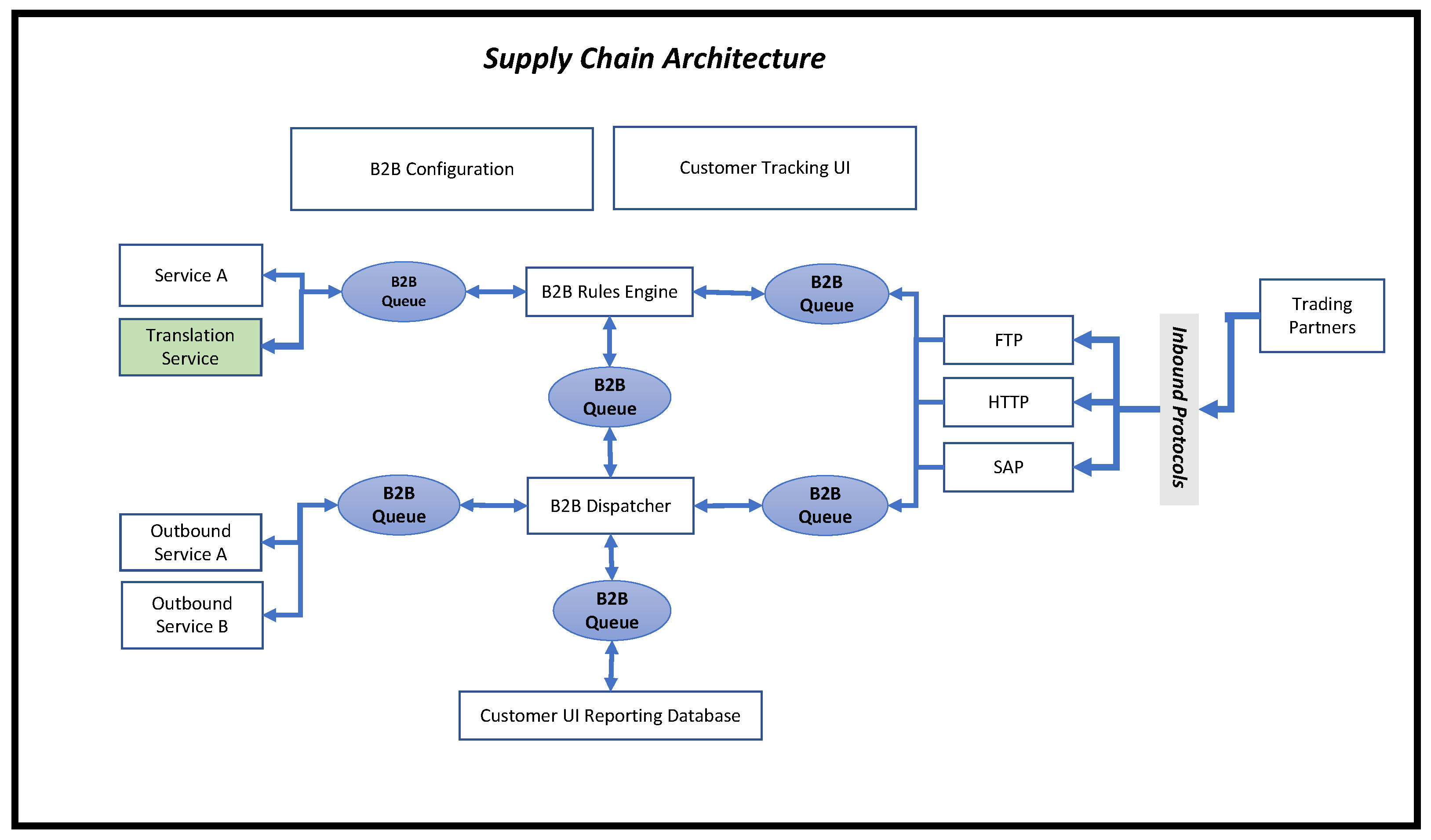
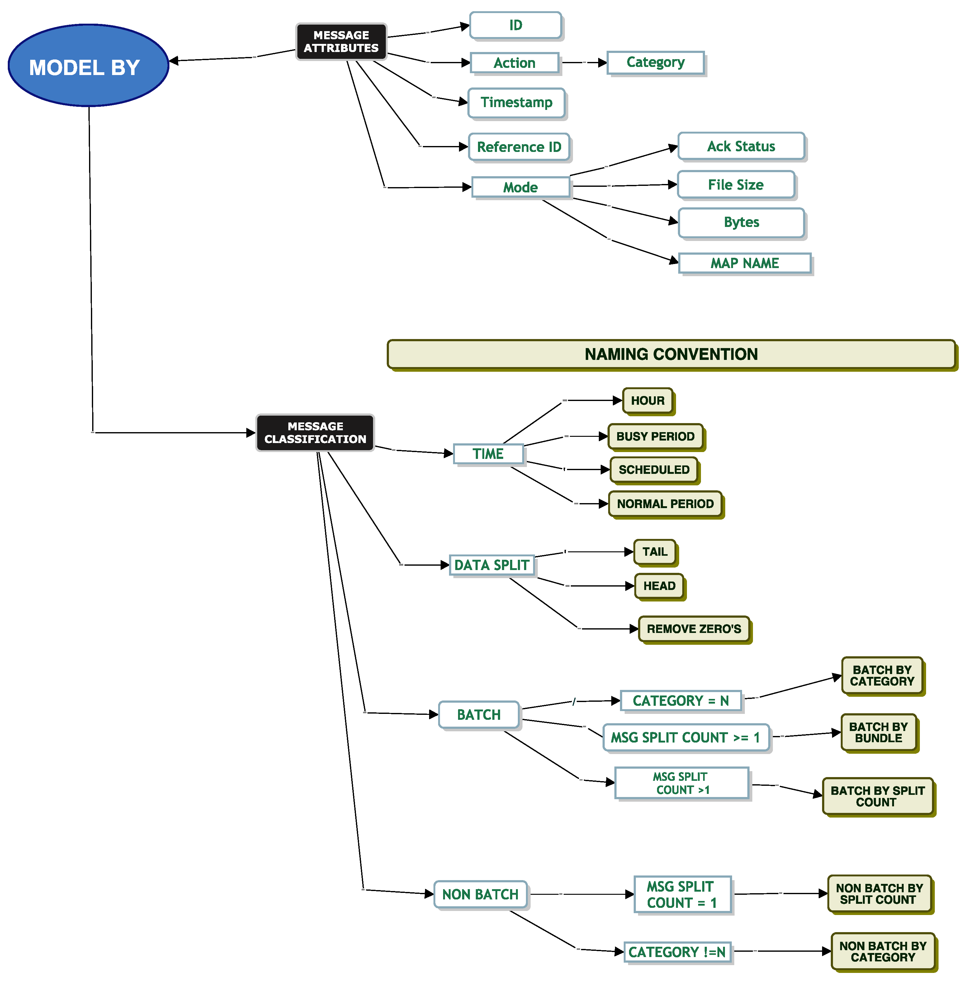
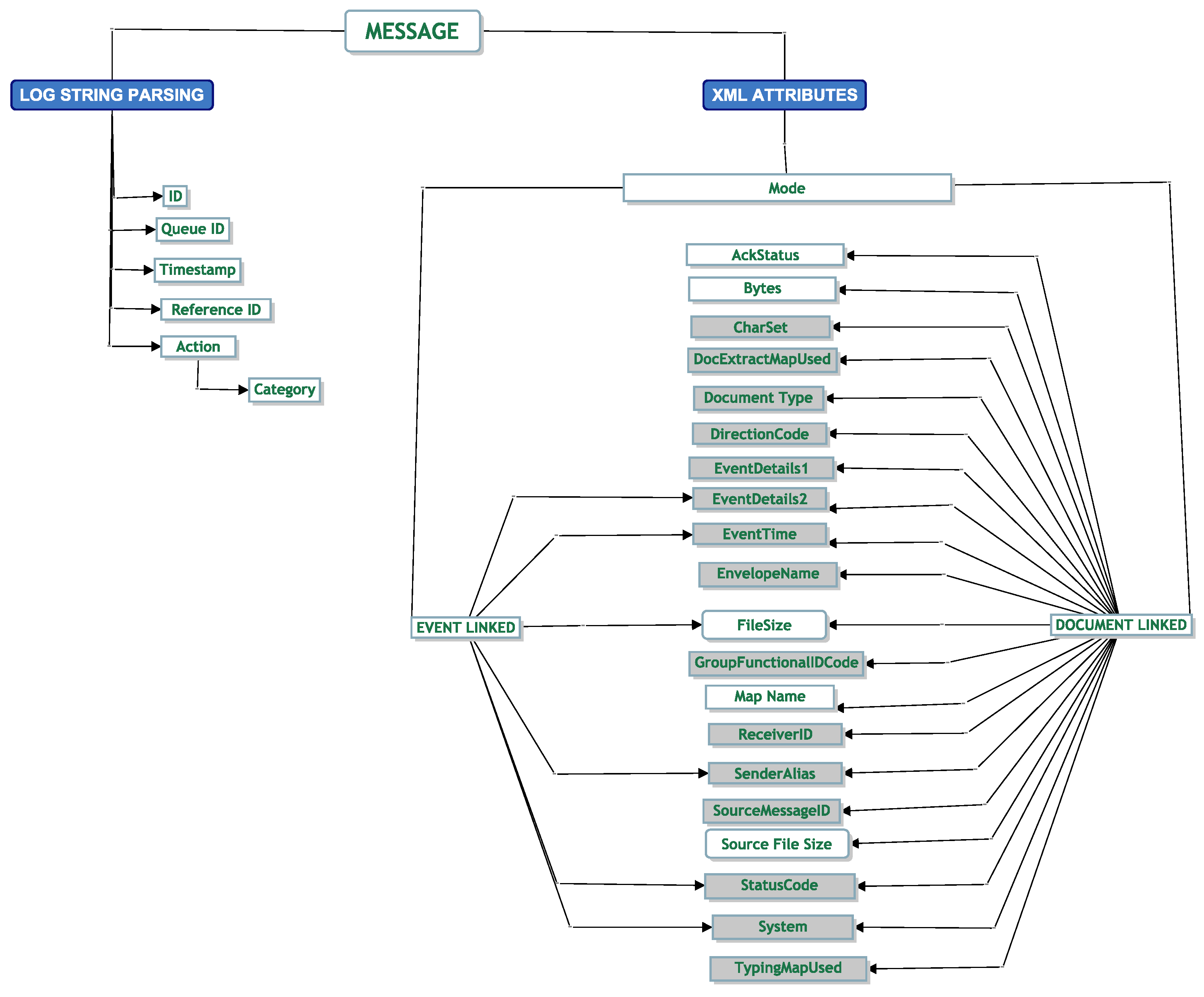
3.2.1. Parametric Modelling

For queue modelling, correlation is a feature that needs to be identified to see if it exists, as queueing models assume no correlation. We have applied extensive studies on these EDI messages around correlation. Please refer to our paper for further reading [11].

When modelling EDI messages, we found many challenges. From these challenges, the classification model was born. The different elements of the classification model helped us answer a challenge we faced. For example, we could not tell what happened to a message as it was being translated. We did not know if a message was dependent on another message. We were challenged with modelling the data with a continuous distribution. We faced many challenges around the removal of correlation and trying to break the head and tail of the data at a suitable point to help parametric fitting.

The classification model helped us iterate through the different techniques to help us address the challenges we faced. Our next set of sections will help bring the reader through our techniques based on these challenges.

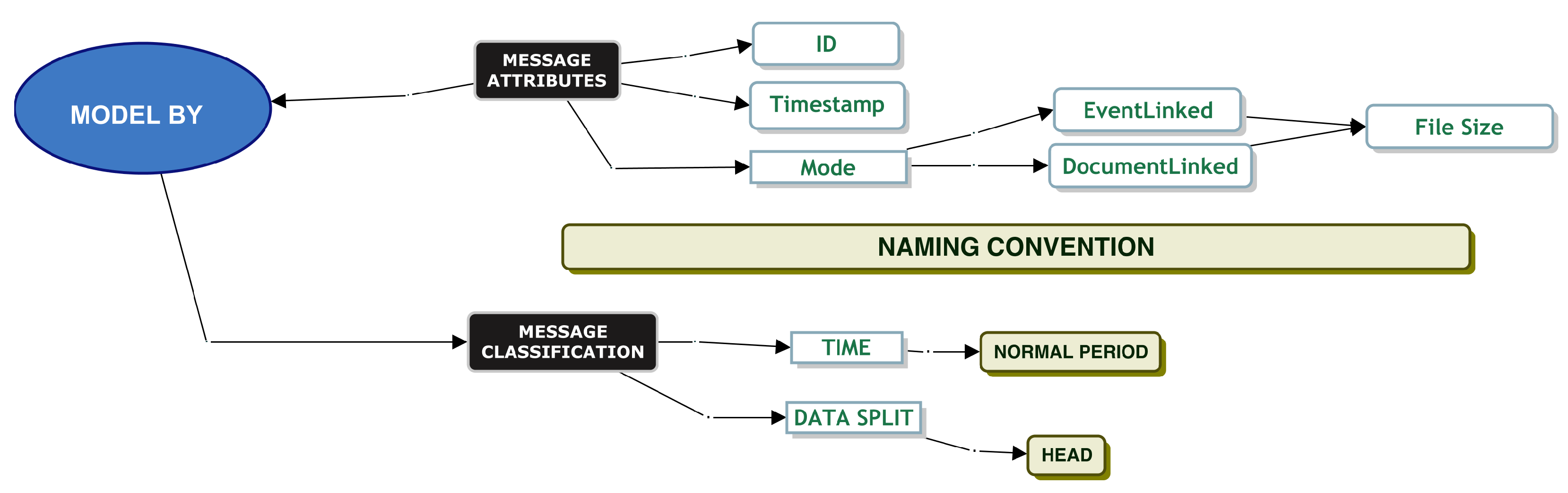
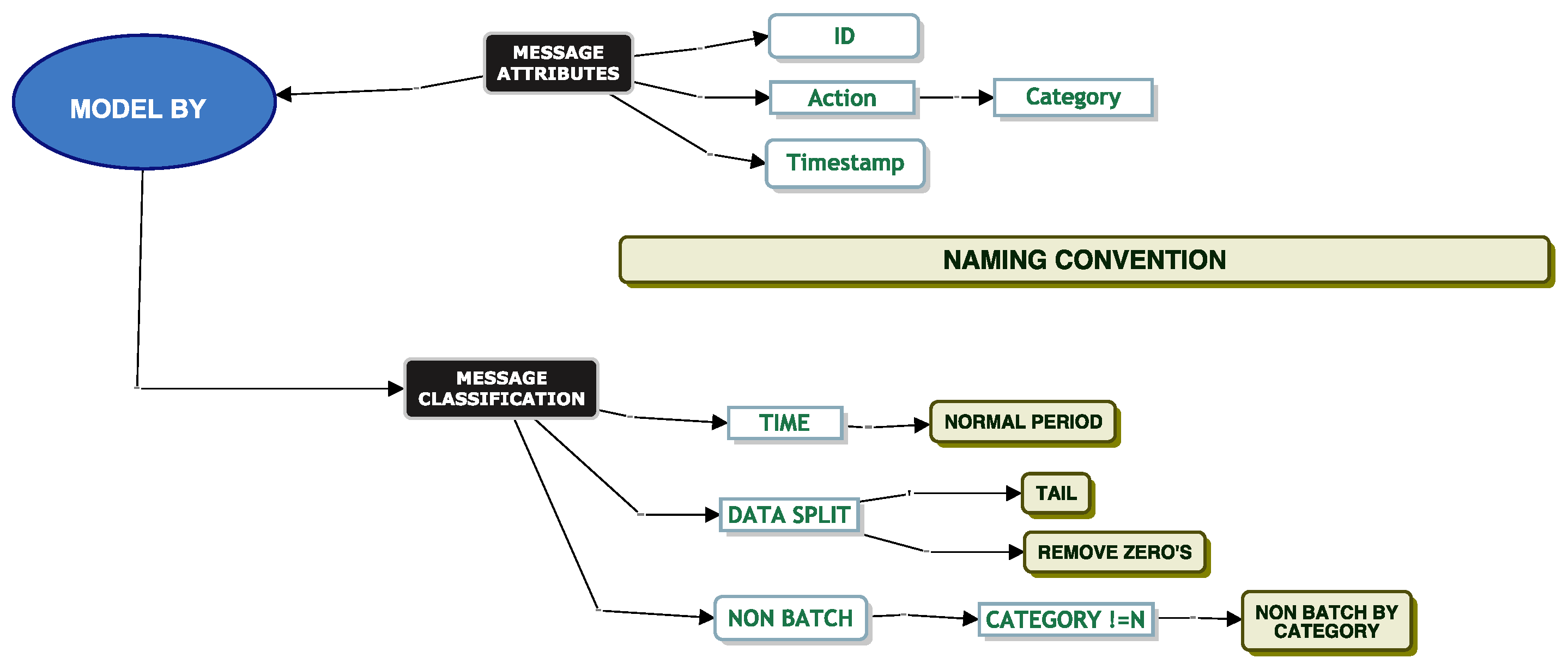
Model By File Size

When testing a system, it is important to understand each message’s file size, as it gives an indication as to whether the message needs to be split for queue ingestion and the amount of disk space required. File size may influence service times. DevOps informed us that one of the inbound connectors does not allow a file size greater than 100 MB, and most file sizes are approximately 20 kilobytes in size.

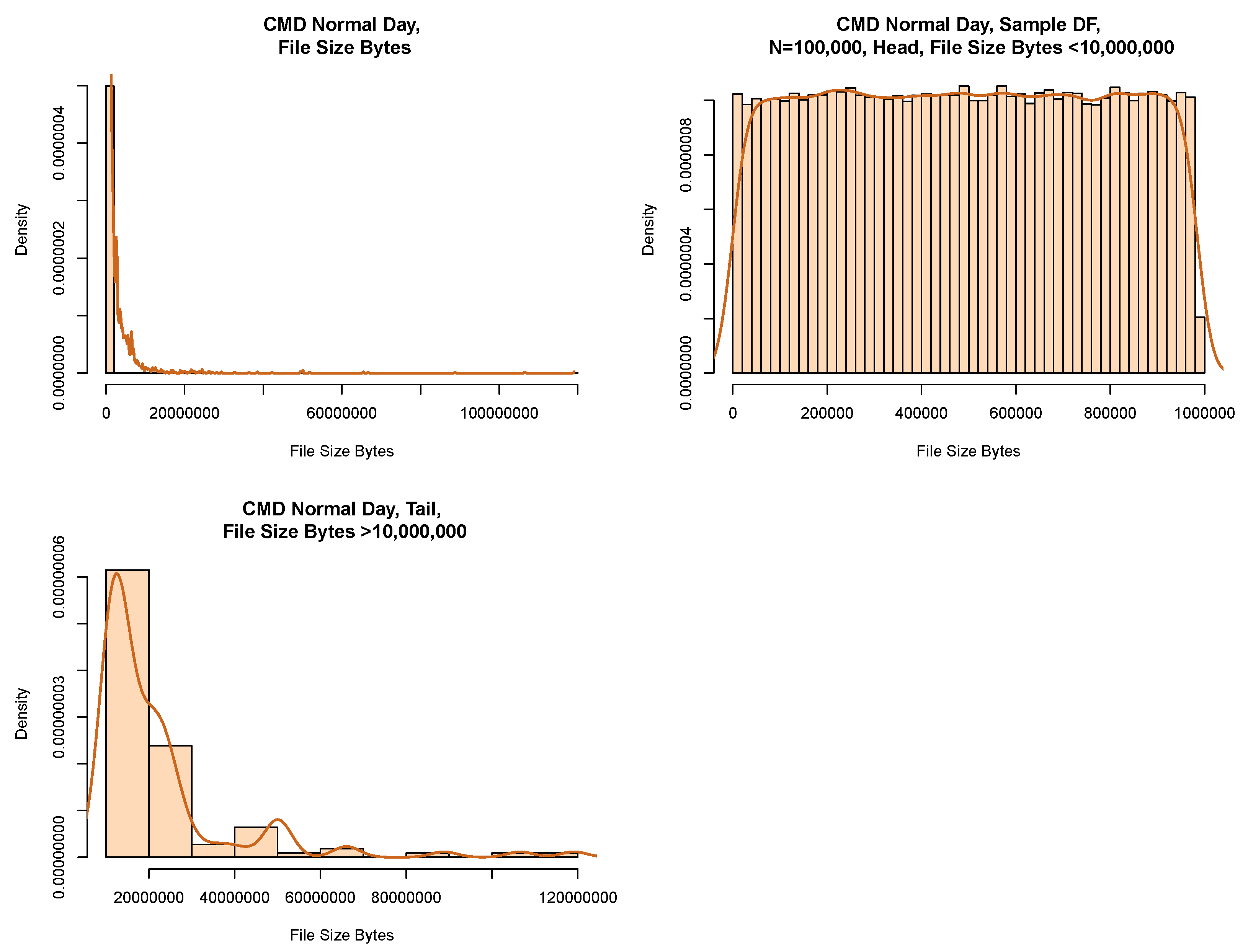
When modelling by file size, we applied the classification model to our data as per Figure 5. Figure 7 displays the model chosen that allowed us to successfully fit a parametric distribution to our data. We picked data from the “Normal Period” and partitioned the data into its head and tail using a size of 10,000,000 B as the boundary. We then took a random sample from the dataset.

Table 7. File size count.

Status	Count
Head	984,070
Tail	109

gives the count of data per partition before we implemented a random sample on the model. We note that we captured the majority of the data in the head.

Figure 8 shows a histogram of our data both before and after the partition. The plot to the top left shows the data before partitioning. The plot to the top right shows the results of a random sample from the head. We can see that the shape of the histogram shows signs of fitting into a uniform distribution. The plot to the bottom left shows the tail of the data.

We use a Chi-square GoF test for the head of the data (see

Table 8. File size, head, Chi-square uniform distribution test.

Test Statistic	DF	a	p-Value
18	19	0	0.05

). This indicates that with $\alpha$ < p-value 0.05, it appears that a uniform distribution may be a reasonable model for the head of the distribution.

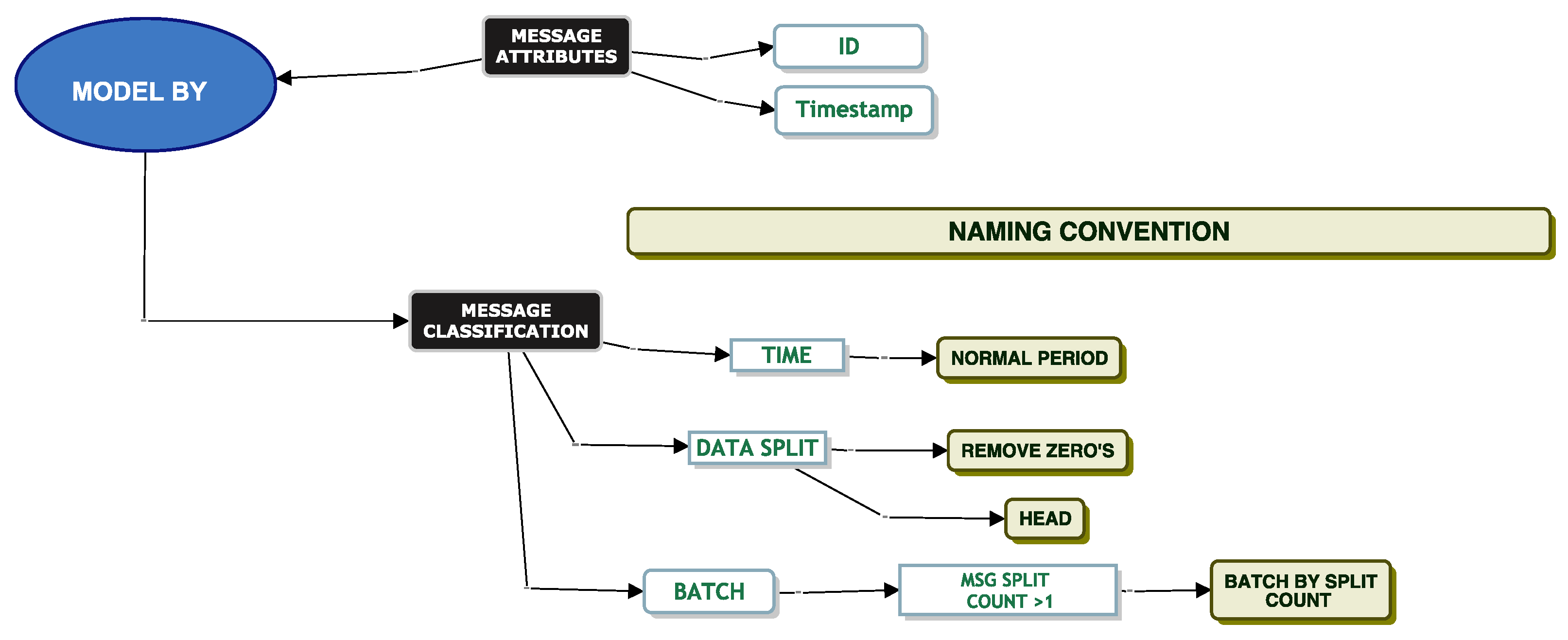
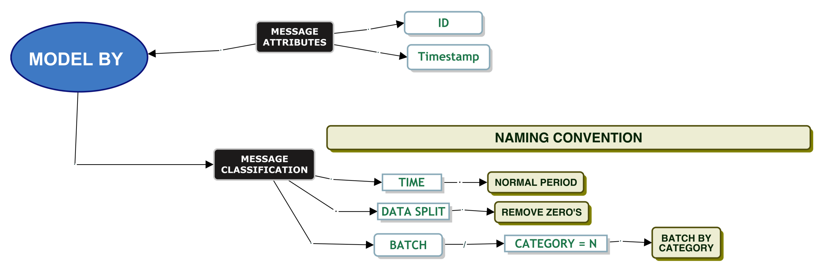
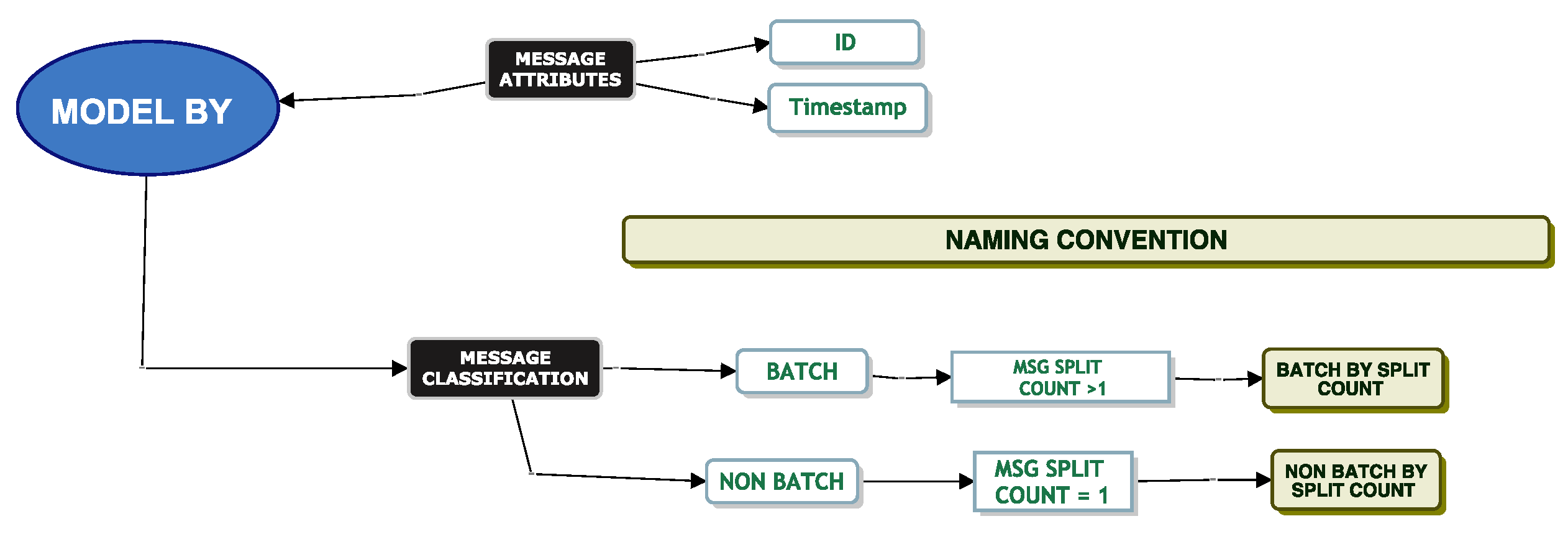
Model Batch By Category

Service Time Modelling

When simulating service and inter-arrival times, it is important to know if the queue will ingest a message as a single message or as a batch of messages. This is because a batch arrival would be a clear type of interdependence between messages that would be relevant for queue modelling. DevOps informed us that certain messages (“Flat Translation” or “Batch Translation”) should be considered batch messages based on their “Category” attribute. These messages should be split into smaller files and sent into the system as a batch. All other messages should be considered non-batch type messages. When we inspected the data, we found evidence that the messages for flat translation and batch translation were both single messages and batch-type messages. Based on these initial comments from DevOps, we went ahead and modelled the service times of these messages.

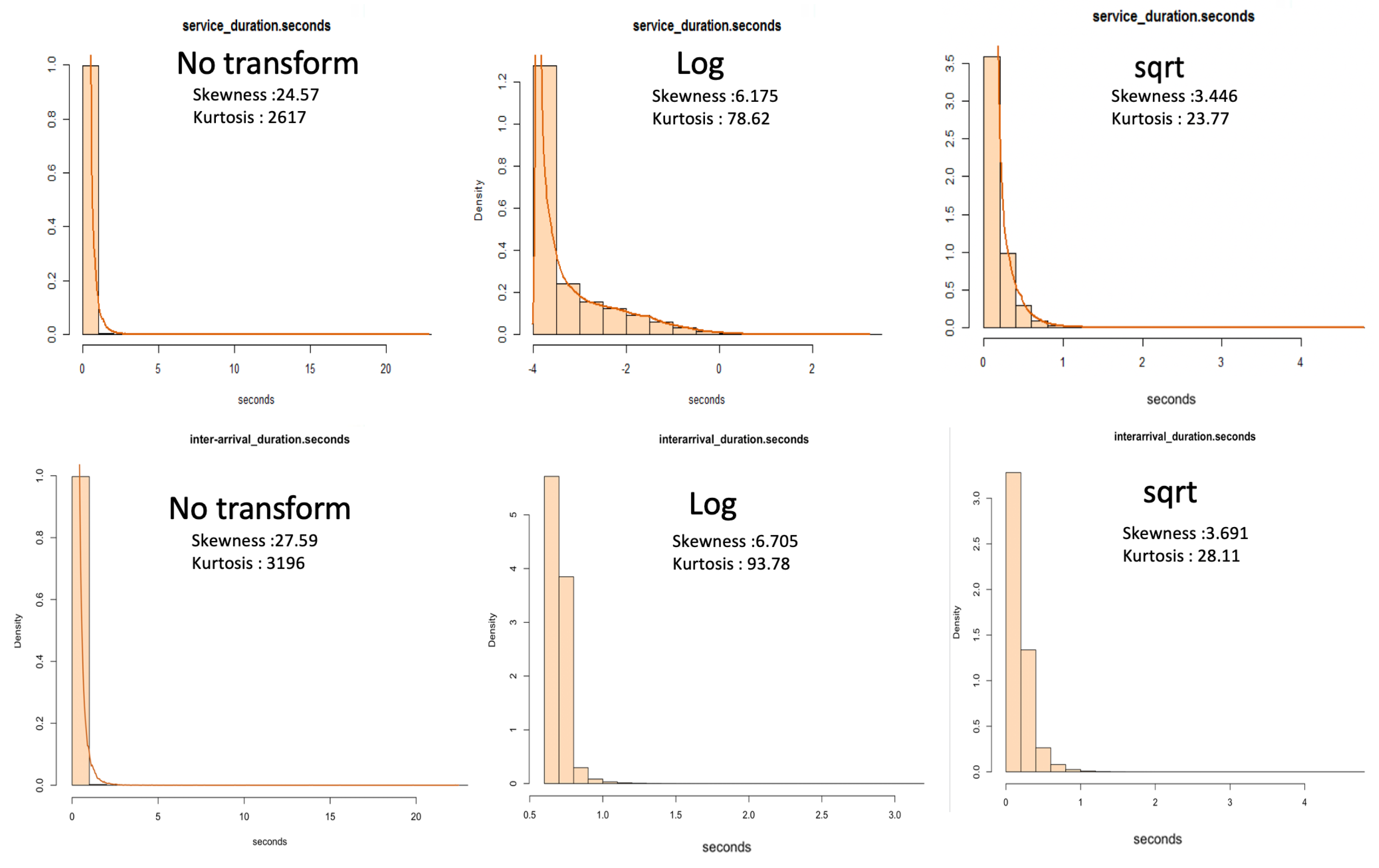
Before attempting to model the service times of the dataset, we analysed measures of dispersion. From

Table 9. Service times, batch by category statistics.

Service Duration Second	Total	Min	Mean	Max	95th Percentile	99th Percentile	Var	Skewness	Kurtosis
Batch	126,742	0	0.03	14.04	0.16	0.44	0.01	26.17	2716
Batch zero removed	65,878	0.001	0.05	14.04	0.26	0.61	0.01	20.84	1658

, we note that of the total batch messages, half of the messages were removed when we removed messages of zero duration. We also observe that these data are heavy-tailed with a skewness greater than 20 and high kurtosis. There is a 0.10 s difference in the 95th percentile between the service times of both batch messages and batch messages where zeros are removed. Messages greater than zero seconds in service times are likely to take less than 0.26 s to process.

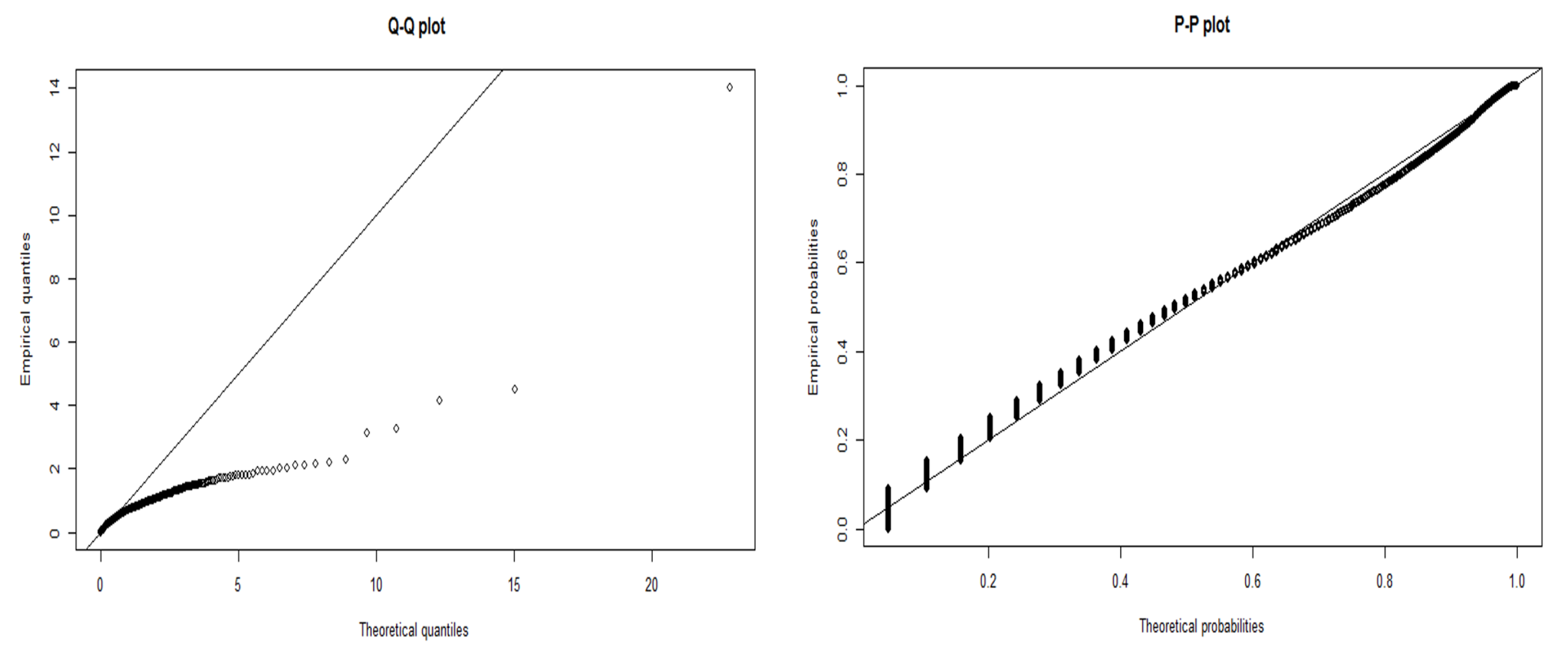
We applied the model from Figure 9 without partitioning the data by head or tail.

Table 10. Batch by category AD result.

Test	Transformation Sqrt	Transformation Cube Root
Burr	362	362
Log-normal	281	281

shows the top two models with the lowest AD score. We note that these data are close to a log-normal distribution but significantly fail the AD test.

To further understand our results, in Figure 10, we compare the data after a square root transform to the modelled log-normal distribution. The Q-Q plot shows that the data tail off at the start of the quantile line. We observe from the P-P plot that while the data appear continuous on the right-hand side of the plot, there are many discrete values on the lower probabilities.

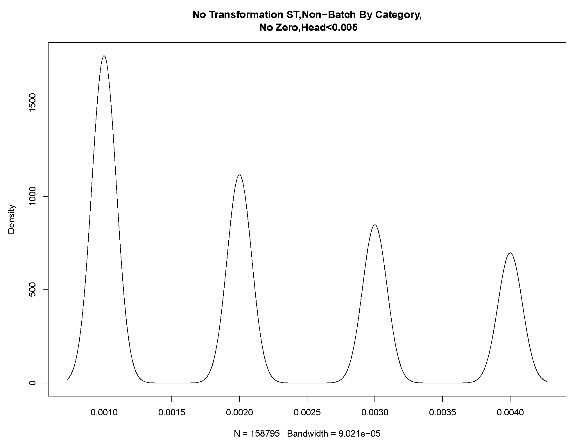
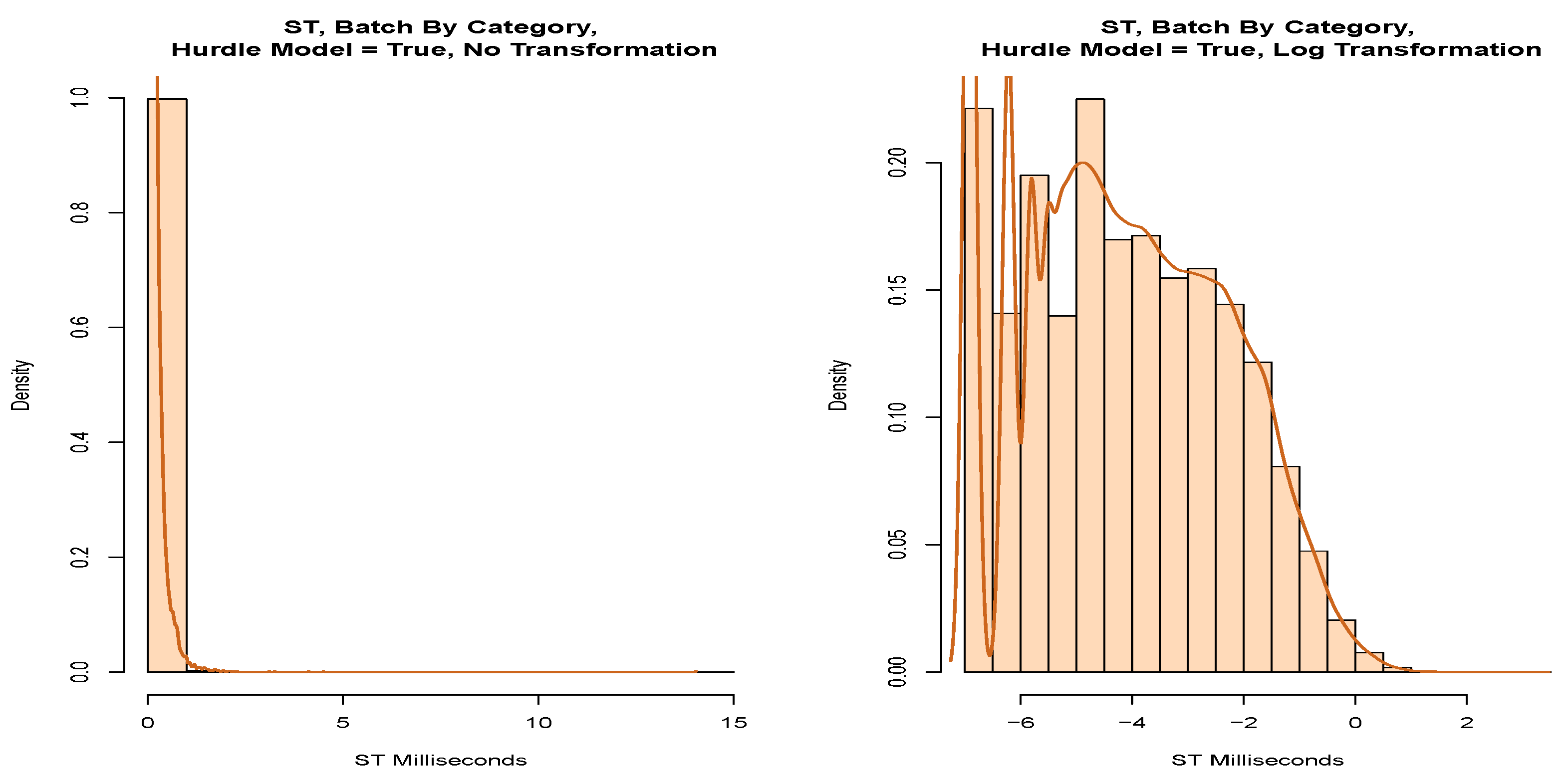
If we partition these data into a head and tail, we find clear evidence of discrete values in the P-P plot shown in Figure 11. From these values, we were able to draw four discrete Gaussian distributions. These four Gaussian distributions result from KDE estimation applied to the discrete data and are not a feature of our data but a feature of the underlying system in the way that the mantissa is set on the message timestamp. We expect our data to be continuous, and this figure and data are not a true representation. We discuss this further in Section 4.4.

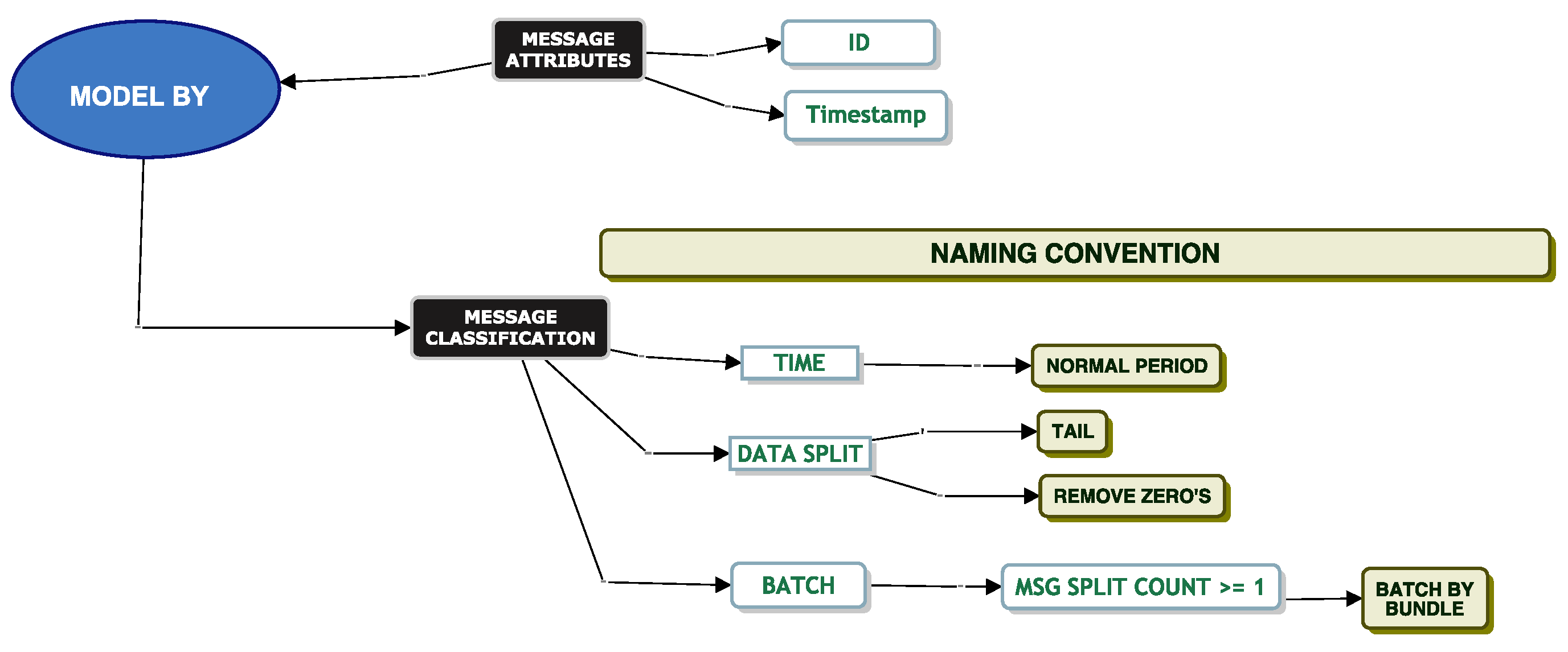
Model Batch By Bundle

Service Time Modelling

In this section, we consider messages that correspond to a bundle of XML documents, which we call “Batch By Bundle”. Our aim is to investigate the fitting of a parametric distribution to the service times accounting for these “Batch by Bundle” messages.

To recap on modelling “Batch By Bundle”, we take all messages and count the number of XML documents associated with a message. If a message has only one XML document, we take the service times for these messages for modelling. For any messages where the XML document count associated with a message is greater than one, we take the first and last message of this bundle and discard all messages in between. We note that all messages in between are all zero seconds in duration.

Using the model in Figure 12, we applied data from the “normal period” using the tail of the data and removing zeros from the model. Our model came close to fitting a log-normal parametric distribution but failed the AD GoF test.

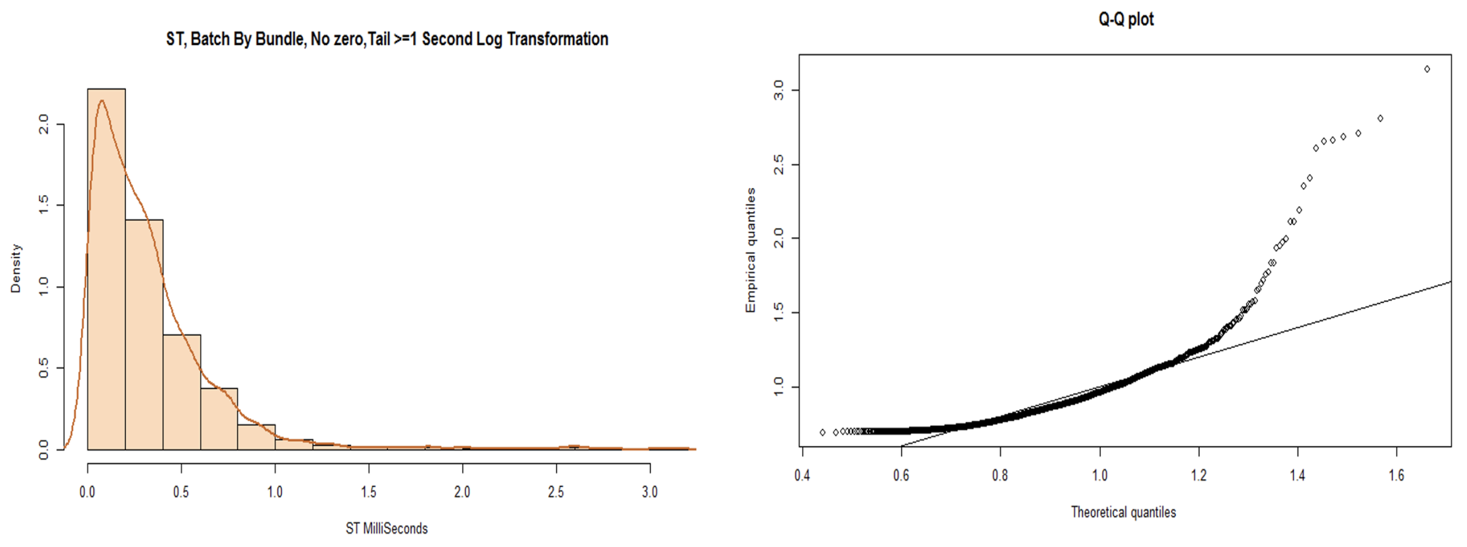
We partitioned the data into a head and tail, using a boundary of 1 s. The model results of fitting the log-normal distribution to the tail of the data are shown in the chart to the left of Figure 13. The histogram represents a shape close to a log-normal distribution but again fails the AD test. The chart to the right shows the results of the Q-Q plot for log-normal distribution fitting. We observe from the Q-Q plot that the lower quantile regions are more fitting to the line than the upper quantile regions, but there are clear systematic mismatches.

Table 11. Tail: AD GoF test—batch by bundle.

Tail Test	AD	p-Value	Transformation	Constant
log-normal	61	0.0000003	Log	1

shows our best AD test result. We applied a constant of 1 to the tail of the service times and applied a log transform on the data to improve the fit.

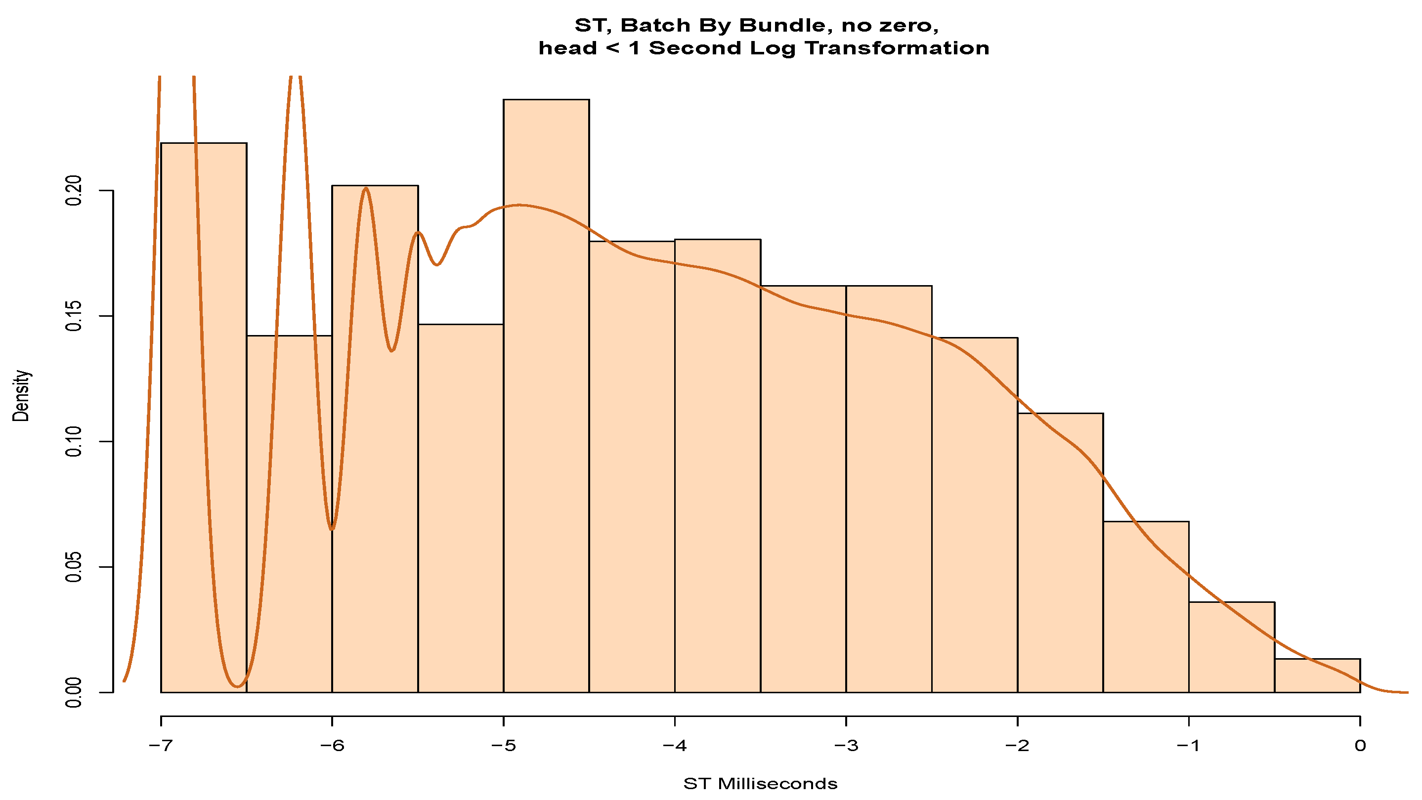
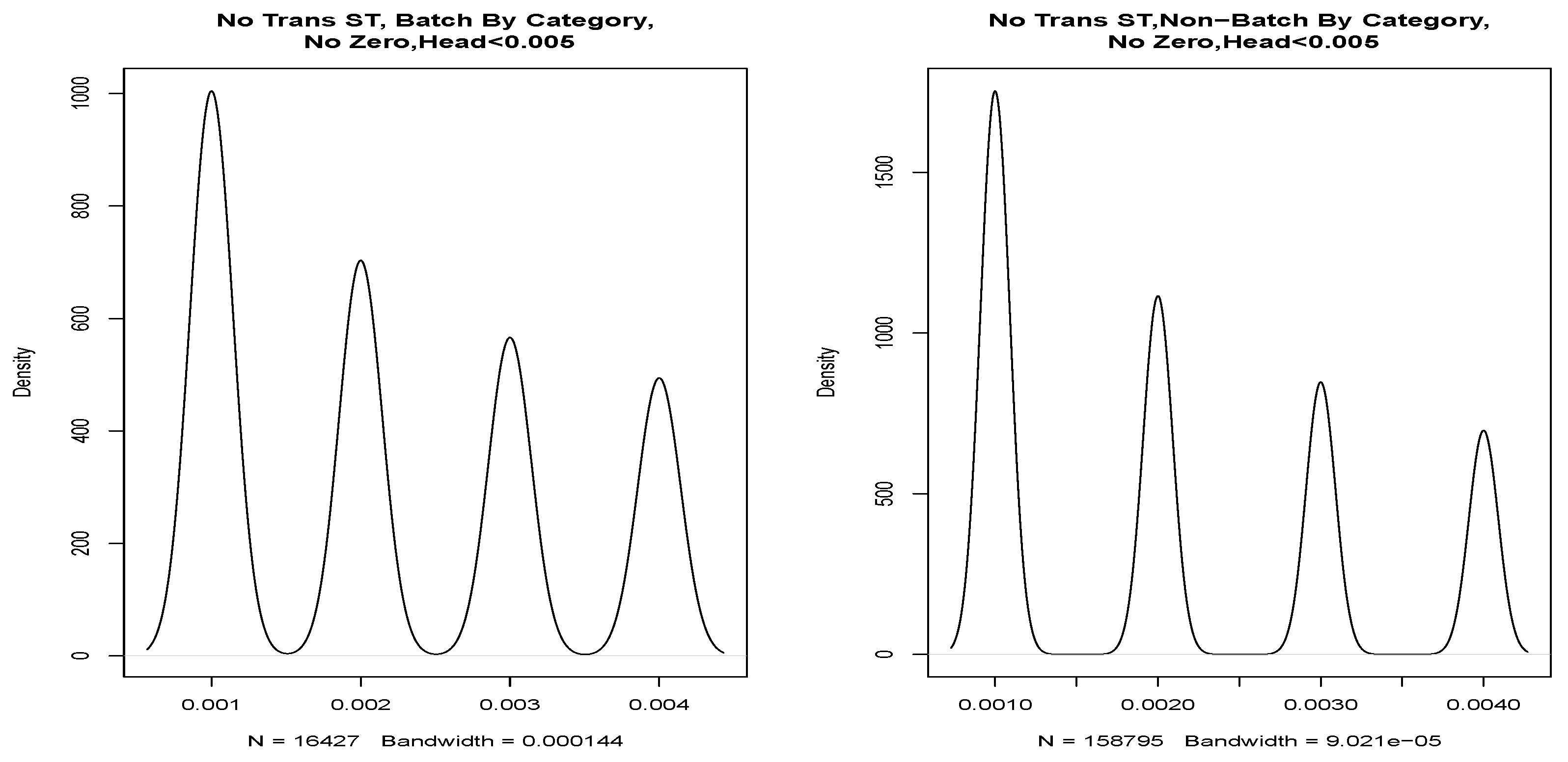
To model the head of the data, Figure 14 shows a histogram with a probability density drawn on the service times. We note several peaks at the left of the estimated density that again suggests quantisation. Consequently, it is unlikely that these data would fit a parametric distribution. Possibly, it could be further partitioned, KDE could be applied, or adjustments could be made for quantisation.

We now attempt to model our data using “Batch By Split Count”.

Model Batch By Split Count

We classify messages using a “Batch By Split Count”. As mentioned previously, one single message may be split into multiple smaller messages and sent to the queue as a batch. A “Batch By Split Count” is one where the XML document count is $>1$. Again, we attempt to fit a parametric distribution to the service times of these messages. We then model the messages using three different partitioning techniques. We model messages where the XML count is $>1$, where the XML count $>2$ and where the XML count $=2$ as per Figure 15.

Regardless of the transformation and partitioning technique applied, we could not fit our data to a parametric distribution to the service times of these batch messages.

Table 12. Batch by split count, ST $\le 1$ second, filter >2, zero removed.

AD Test	Normal	Log(n + 1)	Sqrt(n)	Exp(n)	Exp(log(n + 1))	Sqrt(log(n + 1))	Log(log(n + 1) + 1)	Sqrt(exp(n))
log-normal	39	51	39	1500	1300	51	63	1500
Burr	41	45	41	640	470	45	49	640

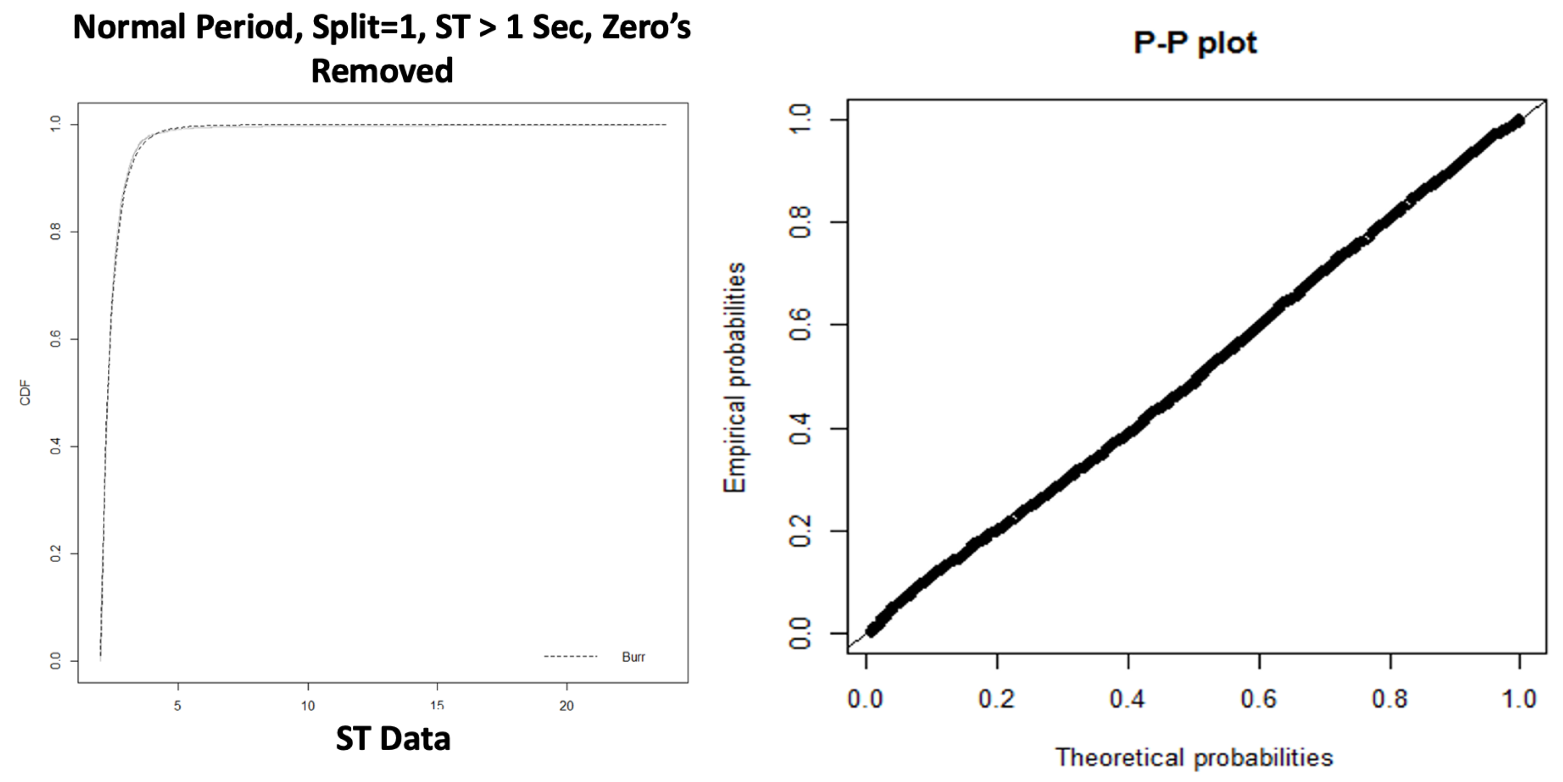
In the interests of space, only AD scores are shown. The majority of p-values rounded to 0.00.

shows the top two distributions with the lowest AD score. If we model the head of the service times, where the split count is >2, the service times is ≤1 s, no transformation is applied, and zeros are removed, our model comes close to fitting a log-normal distribution with an AD score of 39 and also comes close to fitting a Burr distribution with an AD score of 41.

Based on the observations in Table 12, and looking at the results of the applied model for a log-normal distribution in Figure 16, our data do not fit a parametric distribution for the head of the data.

We note that we were also not able to fit the tail of the data to a parametric distribution.

We now focus our efforts on modelling by “Non-Batch By Split Count”.

Model Non-Batch By Split Count

Service Time And Inter-Arrival Time Modelling

“Non-Batch By Split Count” is the complement of “Batch By Split Count”; it considers the messages where exactly one XML document is associated with the message. We modelled the service and the inter-arrival times by applying different techniques of the classification model. The results of our analysis indicate that we could only fit a Burr distribution to the tail of the data, as per Figure 17.

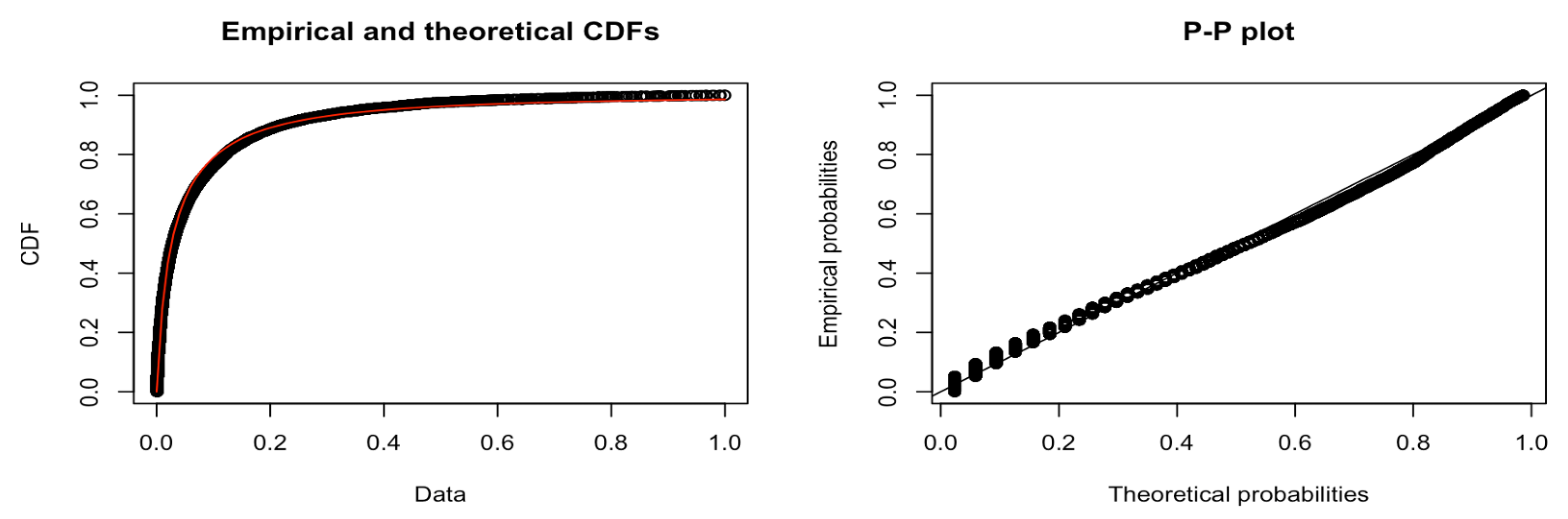
The results of the Anderson–Darling test in

Table 13. AD test normal period, ST, tail of data.

AD Score	p-Value	Test
1.2	0.3	Pass

confirm that we can fit the tail of the service times to a Burr distribution. Note that we applied a constant offset of 1 to the dataset when it passed the AD GoF test. The CDF plot in Figure 18 shows both the empirical distribution and the fitted Burr distribution. From the P-P plot, we note that no observations appear to deviate significantly from the line.

For the head of the service times data (service times $\le 1$ s), we could not parametrically fit the data to a parametric distribution, irrespective of transformation or implementing partitioning methods.

Now we consider inter-arrival times partitioned into the head and a tail with a boundary of 1 s. For the tail (>1 s), the results of the AD tests conclude (

Table 14. IAT > 1 s, Split Count = 1: AD Test.

AD Test	Data	Log (data + 1)	Sqrt (data)	Exp (data)	Sqrt (log (data + 1))	Log (log (data + 1) + 1)	Sqrt (exp (data))
	AD Score
Burr	3.9	6.6	4	Inf	6.6	8.5	Inf

In the interest of space, only AD scores are shown in the table. The majority of p-values round to 0.00.

) that these filtered data do not fit a parametric distribution. However, we observe that a no-transform and a square root transform (highlighted in bold) are a relatively close fit to a Burr distribution but do not pass the AD test. Table 14 shows only the closest model to a parametric distribution. When modelling the head of the inter-arrival times, we found evidence of correlation, which is included in our conference paper [11].

Model Non-Batch By Category

Service Time Modelling

To recap on the importance of modelling by “Non-Batch By Category”, we refer the reader back to Section 3.2.1. We now try and fit a parametric distribution to our data using different techniques from the classification model. First, we analyse the measures of dispersion using the “Non-Batch By Category” model. We note from

Table 15. Non-batch by category measures of dispersion.

Service Duration Second	Total	Min	Mean	Max	95th Percentile	99th Percentile	Median	Var	Skewness	Kurtosis
Non-Batch	857,437	0	0.04	22.81	0.23	0.60	0.004	0.01	24.24	2550
Non-Batch zero removed	570,020	0.001	0.06	22.81	0.31	0.73	0.01	0.02	21.06	1880

that for the service times, one-third of the messages are removed when we remove messages of zero duration. We also note a slight difference in the service times in the 95th percentile between non-batch messages and when zeros are removed from the dataset. Our dataset is highly skewed, with a reporting skewness greater than 20. With the zeros removed from the dataset, the lowest service time is 0.001 s.

Our closest model to fit a parametric distribution is in Figure 19. We apply the model to the “Normal Period” using the “Tail” of the data and removing messages that are zero seconds in duration.

Table 16. Non-batch by category, tail of ST, AD results.

Test	No Transform	Log Transform +1	Square Root	Cube Root
log-normal	3942	3966	3942	3942

shows the top two best models for parametric fitting. We note a large AD score and ascertain that even the best fitting model is not particularly good, and so we have not identified a suitable parametric model.

When modelling the head of our data, we again found evidence of discrete values leading to quantisation noise. We refer to Section 4.4 for a discussion around the effects of quantisation.

Using the classification model, we attempt to fit our data to a parametric distribution. We now focus our efforts on non-parametric modelling.

3.2.2. Non-Parametric Modelling

Where we could not fit a parametric distribution, even after partitioning the data using our classification model, we explored modelling the data with KDE. We know that KDE usually provides a good fit to the observed data, based on the different algorithms and kernels drawn to support each point’s area under the curve. For example, Figure 20 shows an example of fitting the tail of service time data by the hour with KDE. The histogram to the left uses a bandwidth selector of the Sheather–Jones “plug-in” estimator with a method of “dpi” and an Epanechnikov kernel. The histogram to the right has a bandwidth selector of unbiased cross-validation using a rectangular kernel.

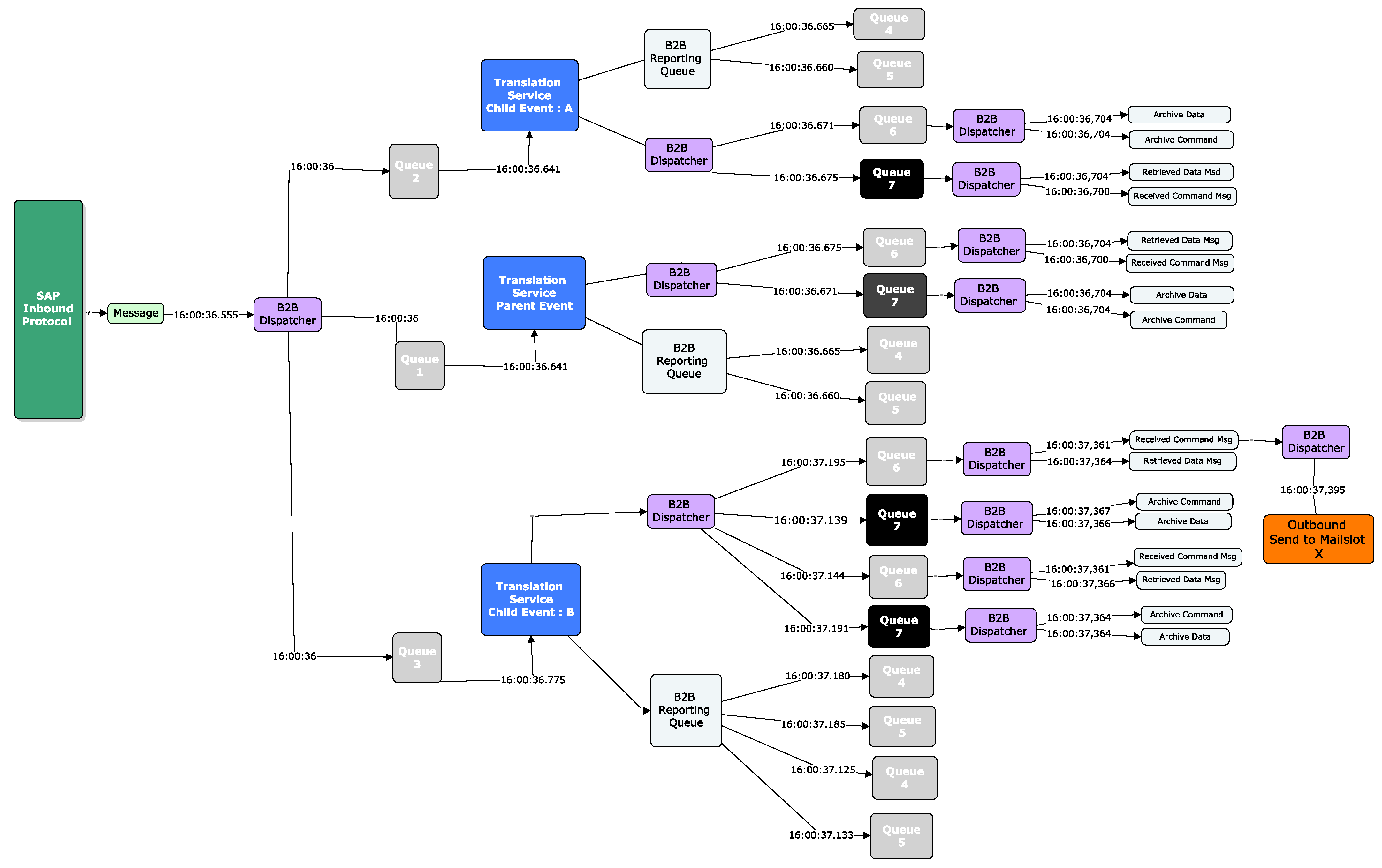
3.2.3. Message Interdependence

Message interdependence is critical when simulating a queueing system. Modelling single message behaviour through a queueing system is less complicated than modelling messages where there is a parent–child relationship, and the relationship may be one too many. The service times of a batch message may not be determined until the last child message arrives and is processed in the queueing system. Using the classification model, we attempted to understand if we could easily identify a parent–child relationship within our dataset. Applying the models from Figure 21, we observe that we were able to determine if a message was dependent on previous messages based on the “Batch By Split Count” model and the “Non-Batch By Split Count” model.

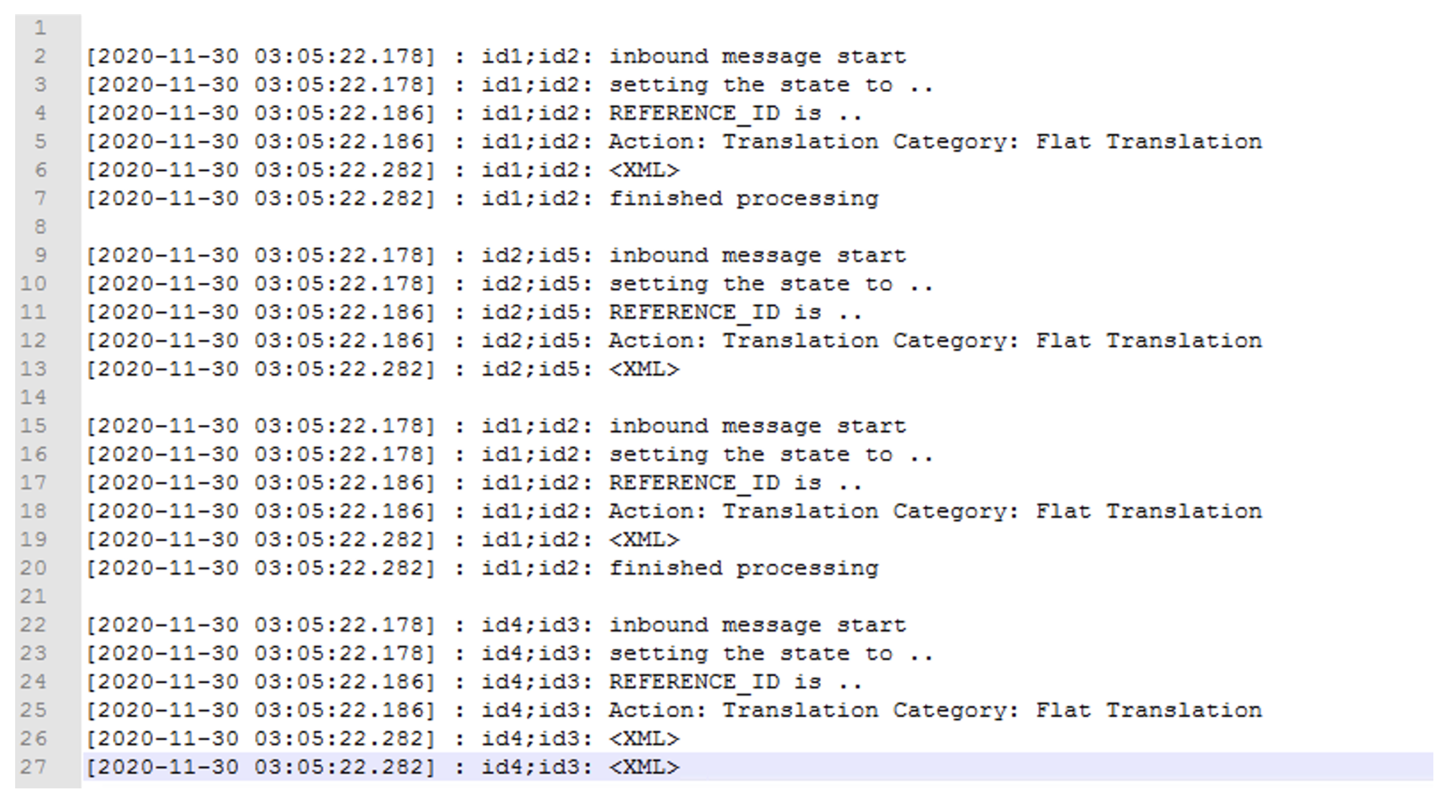
We now explore the text in Figure 22 to give some context on how we came to this conclusion.

At a high-level view, a message first arrives in line 2. The message is set to an associated state defined by a map associated with the message as per line 3, and the customer name is associated in line 4 using a Reference ID. The message is then sent for translation in line 5, and the XML for the message is produced in line 6. The message is then completed processing in line 7. A subset of this message is then processed again starting from line 15 and is finished at line 20. This means that this message is split into two messages and is fully complete at line 20.

In more detail, we took the ID of the message and split the string in two (id1:id2). The first string was the Company ID (id1), and the second string was the Message-ID (id2). Consider the hypothetical example in Figure 22. Using the second part of the ID in the second delimited column (id2), we counted the number of times the message had a string tag of <XML>. We note that the message first enters the system on line 2. It then has an <XML> tag on line 6. We count this as 1 XML document. We then note the message arrives in the system again at line 15, and at line 19, it has another <XML> tag. We count this as 2 XML documents for id2. We iterate through all the log data until the last part of the message comes into the system, and we aggregate the count of <XML> tags.

It is important to note that if there were 2 <XML> tags, i.e., if we had one on lines 26 and 27, we would only take the first <XML> tag as a count. Although we never saw this behaviour in the wild, we note this in case it happens on other systems.

Using the signature, we can now determine if a single arrival will send an influx of messages into the queueing system.

We also seek to understand if there is a dependence between the service times of these independent and non-independent messages. To explore this, we split the messages into messages where the service time exceeds 1 s or 2 s (see

Table 17. ST exceeds 1:2 s.

Classification	ST ≤ 1 s	ST > 1 s	ST ≤ 2 s	ST > 2 s
Independent	126,585	157	126,731	11
Non-Independent	854,722	2714	857,160	276

). We chose these values, as they reflect the tail of our data, and it would be useful to know if these messages are more likely to be in the tail.

We perform a Fisher’s exact test on our data to check for independence.

Table 18. Dependence check: ST exceeds N seconds.

Test	Odds Ratio	p-Value
Exceeds 1 s	2.56	0.0000000000000002
Exceeds 2 s	3.71	0.0000003

of the Fisher’s exact test indicates that there is no significant association [p < 0.05] between independent and non-independent messages, where the service times exceed 1 or 2 s in duration.

3.3. Queueing Problems

From an enterprise dataset, we were able to study the different problems documented in the queue ticketing system.

Table 19. Queueing system problems.

Type	Count	Percent
Unclassified	1900	27
Communication Channels	806	11
Installation	620	9
Security	619	9
Transport Layer Security	566	8
Queue Managers	477	7
Authorized Program Analysis Records (APARs)	458	6
Migration	431	6
Product Documentation	334	5
Replicated Data Queue Manager (RDQM)	256	4
Logging, Recovery	234	3
Connectivity	177	3
Performance	171	2

shows several categories of issues observed within a period of a queueing system’s operation. We observe from the table that 27% of the problems are “Unclassified”. “Communication Channel” related issues are the second biggest hitter at 11% and “Performance” is the lowest at 2%. In this context, the “Communication Channel” is a link between the client and server systems or between two servers. Interestingly 7% of the problems relate to “Queue Managers”.

To determine the extent to which messages are re-processed, we used two message attributes to investigate this. Using the “Company ID” and the “Message ID”, we determined how many distinct messages were re-processed. A message is re-processed by the system if the message processing time exceeds 20 min. In this case, the message processing is killed, and the message is re-sent into the system. Of just over 1 million (1,237,370) messages, we uncovered that only a small minority of messages were re-processed.

Table 20. Re-processed messages.

Reprocessed Times	Messages
1	281
2	6
11	1
51	1

shows the results of our analysis. We note from the table that one message was re-processed 51 times, and most messages are only re-processed once.

When EDI messages traverse through different features of a supply chain network, they go through various transformations. A feature of EDI is a functional acknowledgement (FA). An FA sends back a status message, which serves as an electronic receipt to confirm the delivery of a message. It is sent as a response to other EDI messages received [34]. We sought to investigate which types of status messages are most prevalent. This would allow us to, for example, establish the frequency of malformed messages.

Table 21. Queueing system messages by ack status.

Status Message	Count	Percentage
Accepted	194,255	40.59
Waiting	184,632	38.58
None	97,797	20.44
Accepted With Errors	970	0.20
Rejected	563	0.12
Received	303	0.06
Partially Accepted	32	0.01

gives a breakdown of the results. Interestingly, most of these messages do not suffer from malformation during the EDI process, with only 0.12 percent of messages having a return acknowledgement receipt of “Rejected” and 0.20 percent of messages being “Accepted with Errors”.

Table 22. Messages by ack status and transformation.

Message by Status	Transformation	Count
Accepted	DeEnvelope	194,255
Waiting	Flat Translation	80,819
Waiting	XML Translation	61,013
Waiting	Batch XML Translation	41,154
None	XML Translation	41,198
None	Flat Translation	38,097
None	Batch XML Translation	14,279
None	Send	1570
None	Extraction Translation	1534
Accepted With Errors	DeEnvelope	970
Waiting	Flat Potential Translation	856
None	XML Potential Translation	632
Rejected	DeEnvelope	563
Waiting	XML Potential Translation	463
None	Flat Translation	460
Received	DeEnvelope	303
Waiting	Send	269
Waiting	Flat Translation	47
Waiting	Null	11
Partially Accepted	DeEnvelope	32
None	Flat Potential Translation	25
None	Null	2

allows us to investigate the status message and the associated types of EDI transformations. We can use this to ascertain if certain transformations are more susceptible to errors than others. Messages of the type “Rejected” and “Accepted with Errors” perform the same transformation. The transformation identified is a “DeEnvelope” service. The “DeEnvelope” service identifies the interchange type contained within a message and extracts them to separate messages handled by the business process. A list of the interchanges can be found here [35]. We observe that only a subset of messages returns an acknowledgement receipt. DevOps informed us that only messages classified as outbound from the “Direction” attribute of a message will return an acknowledgement status.

We note that most message transformations have a status of accepted whilst applying the DeEnvelope service. Interestingly, no other types of messages transformations have an “accepted” status. All other types of message transformation do showcase multiple types of statuses, most of them being either “Waiting” or “None”.

Every message is associated with some form of EDI transformation, which is defined by the associated “Action” and “Category”.

Table 23. Message category data dictionary.

Name	Description
DeEnvelope Translation	Identifies the interchange type contained within a message and extracts them to separate messages to be handled by the business process
Flat Translation	One flat file in, many flat files out
XML Translation	Transforms XML to an EDI format
Batch XML Translation	One XML contains many documents which are then split into individual documents
Send	Send a message that has been previously deferred
Extraction Translation	Extraction of a document
Null Translation	Dependent on the “Action”
Flat Potential Translation	Run a preprocessing step on the data to see if it is bad before doing any transformations

shows a data dictionary of some of the “Category”-type transformations.

We note from the table that there are eight different types of translations. Two of the most common translations are DeEnvelope translation and flat translation. The DeEnvelope translation locates the envelope type, for example, an ACH inbound envelope and calls the DeEnvelope business process. It then uses a data extraction tool to write out the data. The flat translation may take a flat file and reformat the transaction according to some standard format, such as X12 or EDIFACT.

3.4. Quantisation Noise

In our enterprise dataset, we noted that the timestamps are given to 3 decimal places and saw evidence that this quantisation is a significant factor in our data. For example, consider when we partitioned the data into “Batch By Category” and “Non-Batch By Category”. As the data were heavy-tailed and the majority of the data fell in the first bin of the histogram (Figure 23), we applied Tukey’s ladder of power and transformed the data. The transformed data (Figure 23) shows several peaks. Naively redrawing the density plot for the head of the service time, we note four distinct Gaussian distributions in Figure 24.

Of course, our data contain four distinct values, quantised to 1 ms. However, the smoothed density plot, which works well for the larger values, represents these values as Gaussian distribution around these discrete values. Because a significant amount of our data is spread between values separated by 1 ms, quantisation noise is an important factor for our data.

4. Discussion

Based on the methods we discussed in Section 2, we discuss the results from our methods from Section 3.

4.1. Framework

We put in place a framework to aid the modelling of our queueing data in order to provide structure for the investigation. The framework helped us clarify the requirements of our analysis and allowed us to manage the information gathering and model selection phase. In general, we believe such a framework will support accountability and reasoning behind the outcomes. Other researchers can use this framework and further refine it.

We now explore the results of our investigations around our framework components via Section 4.1.1—feature: identification–selection.

4.1.1. Feature: Identification–Selection

When modelling EDI messages, we found that different XML schemas were dependent on the “Mode” attribute of the message. We identified 78 elements and selected 23 for analysis. From those 23 elements, we further reduced the elements down to 8.

Further to this, we identified six keywords that we used as part of our modelling decisions based on the structured text of the log files.

Combining both the structured text and the XML documents, our final selection was 14 elements out of 29. We believe we captured the important elements for modelling service times and inter-arrival times of EDI messages. These elements may be useful to other researchers and DevOps when modelling their EDI messages.

We now explore the results of the next component of our framework via Section 4.1.2, feature classification.

4.1.2. Feature Classification

The classification or labelling of combined attributes facilitates more detailed consideration messages, and we chose to do this in a way that we hoped would be relevant to the modelling of the queueing system. For example, from the classification model, we were able to identify a single or a batch-type message.

4.2. Modelling

4.2.1. Parametric Modelling

Model By File Size

We wanted to understand the range of file sizes within the dataset. This could allow the construction of a test suite based on real data and allow us to understand how the different sizes might impact queue behaviour. This would also facilitate the provisioning of disk space for the queueing system. We were able to fit the head of the data to a uniform distribution, which will support the requirements around disk space. The tail of the data seems to contain specific file sizes, suggesting that KDE fitting or some model based on knowledge of customer behaviour might be useful.

We considered that if we could identify batch messages via file size, then possibly batch messages would all be large files that are split into smaller pieces. However, we could not determine from the file size whether messages were split. In particular, as the source file size was an optional parameter, we used other fields to determine this.

Model Batch By Category

We modelled our messages based on the associated “Category” on the advice from DevOps; however, we found that the messages identified by the suggested categories could either be single messages or messages that are split into several messages. Further work is required to try and identify the unique features that support this Classification.

We also investigated fitting a parametric distribution to the message service times when modelling messages matching the “Batch by Category”. The final model that we selected indicated that the data were close to a log-normal distribution but failed the AD GoF test. We noted from the P-P plot evidence of a significant number of discrete values, suggesting that our data’s quantisation may be an issue.

Model Batch By Bundle

In an alternative approach to understanding batches of messages, we chose to model all messages that were part of a bundle by considering runs of messages where only the last message had a service time greater than 0 s in Section 3.2.1. We felt that this might help merge batches into a single arrival. Again, we partitioned the data by head and tail and observed that the tail of the data was close to a log-normal distribution. The head of the data was not suitable for parametric modelling.

Model Batch By Split Count

When we analysed the messages by a count of associated XML documents from a queueing perspective, we ascertained that these messages were indeed batch-type messages, even if they were not all batch-type messages from an EDI perspective. We could not get the data to fit a parametric distribution to the partitions of the data we tried. However, some transformations of the head of the data were close to log-normal and Burr distributions.

Model Non-Batch By Split Count

Here, we considered the messages where the XML count of the documents was one. We were able to fit the tail of the service times to a Burr distribution. The head of the service times may be suitable for modelling by KDE. We also attempted to model the inter-arrival times. If we refer back to our previous paper [11], interestingly, the inter-arrival times showed correlation, and we left modelling these correlations as future work.

Model Non-Batch By Category

Using the “Non-Batch By Category” approach, we could not fit this classification model to a parametric distribution. However, it provided clear evidence of the impact of the quantisation of our dataset on modelling.

4.2.2. Non-Parametric Modelling

While we were unable to model all aspects of our data set with parametric distributions, the partitions of our dataset contain many points and make it amenable to modelling via KDE, at least where quantisation is not a significant problem.

4.2.3. Message Interdependence

We explored some aspects of interdependence via our classification model. For example, we found useful relationships between the ID and the XML document count. We checked for independence between the dependant messages and independent messages to see if they have a relationship with the tail of our service times. We used service times greater than 1 s as a starting cut off point. Our Fisher’s exact test concluded that there is no dependence between these types of messages and the tail of the service times.

We note that we observed correlations when modelling inter-arrival times from our paper [11]. This suggests that care might be required if applying a G/G/1 queueing model.

4.3. Queueing Problems

The classification of our ticketing system gives context as to where the identified problems lie within our enterprise queueing application. The 27% unclassified and another 25% made up of non-queue issues, such as installation, migration, APARs and documentation, equate to over 50% of the total problem tickets. The bulk of these problems may have easy fixes. Communication channels, security and transport layer security make up another 28%. Further investigations may be warranted in the detailed classification of communication channels, security issues and unclassified messages.

We investigated our dataset for evidence of throttling. Within the logs analysed, throttling was always set to zero, meaning that throttling did not occur during the period analysed. We also saw that the frequency of bad messages which cause re-tries was less than 1%. Similarly, when looking at the malformation of messages during the EDI transformation stage, we found less than 1% had issues.

Overall, we saw few problems with EDI transformations and bad message formats in the enterprise dataset analysed.

4.4. Quantisation Noise

Truncation or rounding of timestamps has several implications. Firstly, even if the processing times of the system followed, say, a Burr distribution, then rounding or truncation is applied, the result will no longer follow this distribution. As we have a large number of data points, and a significant number of data points lie around the resolution of 1 ms, this can easily be identified by our statistical tests. Secondly, this might have knock-on effects on the temporal ordering of the events.

We were not initially aware that this quantisation noise would be a significant feature of this dataset. In particular, our technique of partitioning the data by head/tail helped us identify where this modelling challenge was significant in the data. As it is not uncommon for data to be rounded in log files to a resolution, such as 1 ms, we highlight the issue of performing a simple fit of a parametric distribution to such data. Similar challenges are likely to face teams with modelling truncated/rounded data.

On investigating other application log files, we found that many applications either already display 6+ decimal places in timestamps or are moving to do so. We would recommend that DevOps teams consider enabling these higher resolution timestamps on their systems and track typical time intervals that must be measured. For example, suppose our timestamp was displayed up to the nano-second. In that case, our dataset from today might not suffer from quantisation noise; however, if typical job times shorten in the future and approach 1 ns, then finer timestamps would be required to fully track the performance of the system.

5. Conclusions

Our study aimed to build a framework to support queue simulation and performance testing of systems processing EDI messages within a supply chain organisation. Our framework allows for a methodical approach to model queueing systems. Developers and performance engineers can use our framework to identify message elements that contribute to bursty and non-bursty messages by looking at different EDI parameters, which will help determine the impact of such burst on a queueing system. Implementors deploying an AmI service within smart spaces can use our framework to determine under or over-provisioning of resources based on the results of the applied model selection tests. Data scientists and researchers can apply our framework to model parametric and non-parametric distributions. Companies can use our research to help inter-twine existing technology with smart modelling. Our framework provides a helping hand when starting to model these EDI messages. Applying context awareness to our EDI feature selection improves knowledge sharing between Supply Chain processes and their impact on the network and within a Supply Chain organisation. We note, in particular, that our data suffered from quantisation noise, which we believe may be a common challenge in the modelling of queueing data with short-lived jobs.

A number of areas remain open for further study. Further exploration of correlation between messages could be investigated. This might be advanced by looking at other elements of EDI message attributes. This might also improve the modelling of the head of the distributions, though resolving issues around quantised data may also help significantly. In subsequent work, we will investigate the effects of quantisation and correlation that were observed in some parts of this dataset.