Missing Data Imputation in the Internet of Things Sensor Networks

Abstract

The Internet of Things (IoT) has had a tremendous impact on the evolution and adoption of information and communication technology. In the modern world, data are generated by individuals and collected automatically by physical objects that are fitted with electronics, sensors, and network connectivity. IoT sensor networks have become integral aspects of environmental monitoring systems. However, data collected from IoT sensor devices are usually incomplete due to various reasons such as sensor failures, drifts, network faults and various other operational issues. The presence of incomplete or missing values can substantially affect the calibration of on-field environmental sensors. The aim of this study is to identify efficient missing data imputation techniques that will ensure accurate calibration of sensors. To achieve this, we propose an efficient and robust imputation technique based on k-means clustering that is capable of selecting the best imputation technique for missing data imputation. We then evaluate the accuracy of our proposed technique against other techniques and test their effect on various calibration processes for data collected from on-field low-cost environmental sensors in urban air pollution monitoring stations. To test the efficiency of the imputation techniques, we simulated missing data rates at 10–40% and also considered missing values occurring over consecutive periods of time (1 day, 1 week and 1 month). Overall, our proposed BFMVI model recorded the best imputation accuracy (0.011758 RMSE for 10% missing data and 0.169418 RMSE at 40% missing data) compared to the other techniques (kNearest-Neighbour (kNN), Regression Imputation (RI), Expectation Maximization (EM) and MissForest techniques) when evaluated using different performance indicators. Moreover, the results show a trade-off between imputation accuracy and computational complexity with benchmark techniques showing a low computational complexity at the expense of accuracy when compared with our proposed technique.

1. Introduction

The rapid increase in the use of IoT technology has resulted in a vast amount of data being collected, mostly from sensor devices. The IoT relies on data collected by various end devices, and data is collected instantly by physical objects that incorporate sensors and network connectivity [1,2]. As a result, there has been a huge surge in the amount of data being generated and sent over the internet. When handling large amounts of data, it has become rather usual to come across large amounts of missing values in the data. Sensor data frequently contains missing values due to data collection and transmission errors [3]. Due to common-mode failures, data with missing values continues to emerge as a long-standing difficulty in the IoT architecture, potentially resulting in bias and loss of precision. These systems rely on data analytics applications that make decisions based on end device data.

It is apparent that educating industrial users about the importance of owning intellectual property (IP) and identifying the merits of continuous development is the best way to increase their interest [4]. There has also been a constant threat of security breaches which could breach the ownership of IP, increasing the risk to established business models. This is especially true when considering IoT-enabled healthcare systems, and that is an excellent demonstration when designing distributed IT systems with comparable complicated needs and stakeholder requirements [4].

Atmospheric pollutants in urban areas are considered as a main factor that has led to the increase in respiratory sicknesses among citizens. Some of these pollutants, e.g., benzene have previously induced cancers when citizens are exposed for prolonged period of time [5]. Hence, it is important to accurately estimate the distribution of these pollutants as it is relevant for traffic management and assists in the design and mobilization of plans to tackle these problems.

Currently, air pollution monitoring in urban areas is essentially carried out using networks of fixed stations that are spatially distributed. These stations can accurately and selectively estimate the concentration of various atmospheric pollutants using Low Cost Sensor (LCS) devices. However, it is sometimes challenging to adequately deploy these networks due to their size and cost [5,6].

It has become possible to acquire spatio-temporal data variables for urban atmospheric pollutants by making use of LCS that are strategically placed in polluted areas. However, the data collected by these sensors are exposed to numerous issues such as drifts, bias and loss of data due to equipment failures [7]. The issue of missing data is a prevalent problem that affects most sensor network domains and other real-life datasets such as traffic [8], medical/health record systems, geo-informatics [9,10], and industrial applications [11].

If missing data is not handled correctly, it can have a significant impact on the veracity of data-based insights. By minimising the sample size and thereby introducing bias, it may limit the study’s final results [12].

Complete Case Analysis (CCA) and missing data imputation are two popular approaches for handling the issue of missing data in research. The goal of the CCA method is to discard instances of a given variable that has missing values. Although, this method is quite straight forward and easy to implement, it leads to loss of data which may hold some useful information. According to [13,14], applying the CCA method will only be useful on a dataset with a large number samples and significantly low percentage of missing data. Imputation on the other hand involves filling in missing values with estimated values.

There are two categories of missing data imputation: (i) single imputation and (ii) multiple imputation. The single imputation approach simply fills in missing values using a single and unique value, e.g., zero value, mean or mode of a given distribution. Multiple imputation however is a model- based technique that is further classified into two: Discriminative (such as Multiple Imputation by Chain Equations (MICE) [15], matrix completion [16] and random forest imputation (missforest) [17]) and Generative multiple imputation method consists of Deep Learning (DL) techniques such as Neural Networks (NN) [18], Generative Adversarial Networks (GAN) [19], and Variational Auto Encoders (VAE) [20]. In this study, we evaluate the consequence of incomplete/missing values on data generated from Low-cost environmental sensors and propose a Best Fit Missing Value Imputation (BFMVI) model based on data clustering for the missing value imputation process. We compare the effects of our suggested technique on sensor calibration to state-of-the-art techniques.

The rest of the paper is laid out as follows: In Section 2, we present our motivation and the contribution of this paper. Section 3 identifies recent research that has been carried out with regards to missing data imputation for sensor calibration. Section 4 presents our experiments and results, clearly describing the dataset used for simulations and our proposed approach. Imputation techniques and their effects on sensor calibration are discussed in Section 5. Lastly, Section 6 concludes the paper and suggests some areas for further research.

2. Motivation and Contribution

The presence of missing values in datasets is a pervasive issue that has drawn attention from various research domains such as medical research [10], data compression [21] and sentence generation [22]. These collaborative efforts have led to the development of state-of-the-art machine learning techniques for solving this issue in datasets with unique characteristics. Our work follows the imputation paradigm presented in [23]. However, this study showcases various improvements to the work done by the previous authors. To further improve the accuracy of the final imputation result, we use stronger predictors and consider the covariates in our imputation model to generate and replace missing values with multiple imputed values rather than single imputed values in each group in order to preserve the variability of the data as opposed to the work in [23]. This study also improves on previous works by testing higher rates and different mechanisms of missing data and presents the efficiency of imputation techniques on machine learning tasks.

In this study, we investigate the performance of various missing data imputation techniques for sensor networks in environmental monitoring stations. During data collection, sensor devices may fail or run into errors which results in the issue of missing data. Consequently, this will have an impact on the advanced analysis of the data collected by these sensor devices [24]. Traditional methods for handling this issue involves deleting instances of a dataset with missing values before proceeding to further analysis. This method is impractical because it totally disregards scenarios with missing values and fails to account for the complex distribution of environmental data, resulting in bias and imprecision [24]. It is possible to impute missing data by learning from the observed data and filling-in missing instances with single or multiple plausible values.

The authors present a novel clustering based approach to missing value imputation for univariate missing data with varying missing patterns. This paper’s main contributions are summarised below:

• As various imputation techniques exist in the literature, when faced with real-life missing instances where there is no ground truth data, it is important to have imputation approaches that will embed the capability of selecting optimal algorithms for imputing missing values. We propose an imputation algorithm called BFMVI that is capable of choosing appropriate techniques for filling-in missing instances based on the nature and characteristics of the missing data.
• We also propose a reverse error score function RES(r) that is based on double Root Mean Squared Error (RMSE) calculations on two final imputation estimates to obtain the final imputation result for filling in missing instances.
• We experimentally demonstrate that considering highly correlated auxiliary variables in the imputation model will impute efficient predictors which will significantly improve the RMSE and MAE scores.
• Our proposed BFMVI algorithm shows a better performance as opposed to alternative benchmark techniques when missing values occur at different rates and consecutive periods of time.

In order to exploit the merits of low latency, high energy efficiency, lower bandwidth consumption and improved data privacy, we suggest the application of the proposed method on the network edge. Bringing imputation algorithms to the edge makes it possible learn more about the dynamics of the urban systems and explore the potential of the generated data.

3. Related Works

The classification of missing data mechanisms is important as it assists in the selection of suitable strategies for handling different missing data problems. According to [25], three important mechanisms of missing data exists namely; Missing at Random (MAR), Missing Completely at Random (MCAR) and Not Missing at Random (NMAR). In the MAR mechanism, the probability of a missing value on an attribute Y depends on the value of another attribute X but not on the value of Y itself [26]. The MCAR mechanism can be noticed when the value of an attribute with missing data neither depends on the missing data nor observed data. MCAR is a mechanism that is considered in most fields to be "totally and randomly" missing. Here, the probability of an attribute Y to have missing values is not directly associated with the output of the variable X or the output value of Y itself [25]. Contrary to previous missing data mechanisms described, assuming we have an organised data matrix, when the chances of missing values on a given attribute Y depends on Y itself, and not the value of another attribute X, data is said to be not missing at random (NMAR) [27].

The Expectation Maximization (EM) algorithm for missing data imputation was proposed by [28]. This is a well known missing data imputation strategy identified in the literature. When imputing missing continuous data, the EM algorithm first evaluates the mean and covariance matrix from the values that are present in the dataset. The algorithm then iterates until there is no significant change to the mean value and covariance matrix as the algorithm moves from one iteration to another. Research has shown that the EM algorithm only works best when data is missing at random. A disadvantage however, is that the EM technique largely depends on information obtained from other variables in a dataset. Therefore, more reliable missing data estimates can only be obtained from highly correlated data using the EM algorithm [23].

In [29], Zhang et al. approached missing data imputation by splitting a dataset into k distinct clusters in the first step. This method results in the generation of membership values for all the points that fall within a specific cluster or centroid. After that, all the missing instances are assessed using the membership measure of other points that fall within the boundary of the same cluster centroid. This technique constitutes an advantage due to its simplicity. However, the predictive accuracy of imputation results from FCM may be influenced by unusual clustering circumstances where the selection of an optimal number of k clusters is a challenge for data miners. An iterative imputation method was also developed by [17], based on the random forest (missForest) method. The idea behind this method involved averaging several regression and classification trees that were unpruned. Their Analyses were conducted on multiple datasets obtained from biological fields, and artificial missing values were simulated on their datasets in order to test the accuracy of their imputation method against different rates of missing values. Their work showed the ability of the missForest method to handle continuous and categorical missing data. Comparatively, after analysing the performance of missForest against some other methods such as KNN, their results showed that missForest outperformed other imputation methods, especially in settings where non-linear relationships and complex interactions were suspected in the dataset.

Gupta et al. [30] approached missing data imputation using Neural Networks (NN) to solve classification problems. The researchers proposed a solution to rebuild missing values using a backpropagation algorithm. Results showed that reconstructing missing values using NN yielded better results than statistical methods. Further analysis also showed that reconstructing missing values using NN improved classification accuracy. Ref. [31] also investigated the performance of missing data techniques on various tasks including regression, classification and bankruptcy prediction using Auto Associative Neural Networks (AANN).

Ref. [32] developed a novel methodology for missing data imputation during the data acquisition phase. In their approach, the authors distributed computation among a range of stationary and mobile devices based on the edge computing paradigm, allowing the network to efficiently scale horizontally, thereby increasing the number of sensing devises and reducing the effect of missing values caused sensing errors.

Various other methods have been proposed in previous research for sensor calibration. De-Vito et al. [5] developed a sensor calibration method based on Neural Networks (NN) using on-site data for $CO$, Benzene, $N{O}_x$ and $N{O}_2$ pollutants in a municipal air quality monitoring station with the use of solid state LCS collected over a 13 months period. Their research showed the viability of achieving neural calibration, which will allow sensor devices to successfully estimate environmental pollutants with optimal results over a bounded amount of training sessions.

Spinnelle et al. made use of Artificial Neural Network (ANN), Simple Linear Regression (SLR) and Multivariate Linear Regression (MLR) to calibrate a group of LCS ($O_3$, $N{O}_2$, NO, CO and $C{O}_2$) over a calibration period of two weeks [33]. Uncertainty measurements estimated by the regression of sensor and ground truth data showed that ANN was a suitable model for calibrating sensor clusters. On the contrary, SLR and MLR yielded measurements with high levels of uncertainty.

4. Experiments

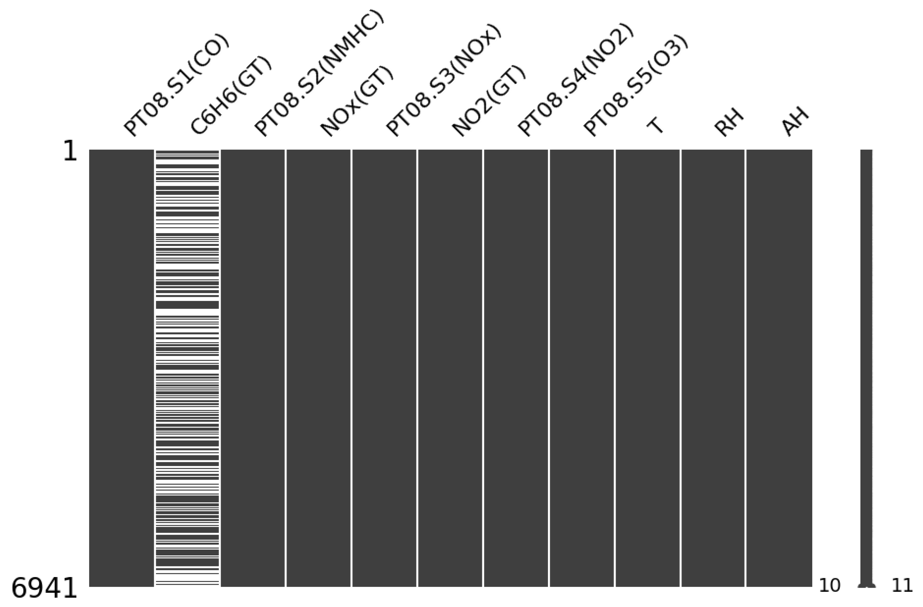
4.1. Dataset Description

For the purpose of our simulation, we made use of a dataset presented by De-Vito et al. [5], which is publicly available on the University of California Irvine (UCI) repository [34]. The dataset contains the concentration measures of target pollutants collected from a measurement site. These concentration values were used as a benchmark to tune a regression system that was designed to calibrate the response of the multi-sensor device. This device was configured to accommodate five metal oxide sensors and two solid state sensors to capture data on the temperature and relative humidity in the environment. The specified station provided concentration estimation values for CO (mg/m${}^3$), C${}_6$H${}_6$ ($\mathsf{\mu }$g/m${}^3$), non-metalic hydrocarbons (NMHC) ($\mathsf{\mu }$g/m${}^3$), NO${}_2$ ($\mathsf{\mu }$g/m${}^3$), NO${}_x$ (ppb). The data was sampled, showing hourly averages of the concentration results. However, the NMHC analyser went offline after 8 days causing a series of missing data. Hourly average values of the multi-sensor device was sampled, showing concentration levels indicated by NO${}_x$, CO, O${}_3$, and NO${}_2$ metal oxide (MOX) chemiresistors in addition to relative humidity and temperature sensors. More information on the MOX chemiresistor is presented in a research by [5].

The original dataset contains real missing values on all columns ranging from as low as 3.91% to a high of 91%, with the highest rate recorded from the GT sensor which we disregarded in our analysis. Assessing the accuracy of imputation methods would be impossible if the dataset is analysed with real missing values present. Therefore, we employed CCA to generate another dataset with fully observed values and created artificial missing values to assess the strength of the imputation techniques on different rates of missing data. An outline of the methodology is clearly described in the following section.

4.2. Methodology

We created different rates of artificial missing data on the variable containing the concentration of C${}_6$H${}_6$ (see Figure 1) and employed single and multiple imputation techniques to replace the uni-variate missing data.

The techniques we considered in this research include EMI, KNN, MissForest, Regression and BFMVI. In order to assess the performance of the algorithms, we follow the approach that was proposed in [35], outlined as follows:

(i)

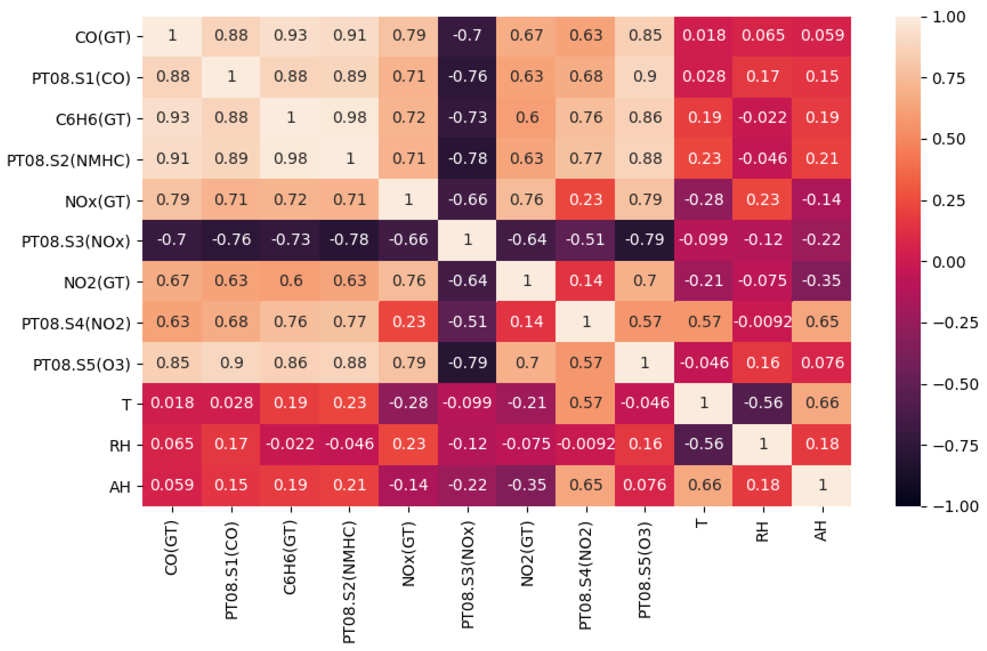
We evaluated the correlation between each feature as seen in Figure 2; features that exhibited strong correlation with the variable (C${}_6$H${}_6$) that required imputation were used in the imputation model.

(ii)

We created missingness at arbitrary points on the target variable.

(iii)

We imputed missing values using the different imputation techniques.

(iv)

The accuracy off all the imputation techniques were assessed and compared using their Root Mean Squared Error (RMSE) indicator.

(v)

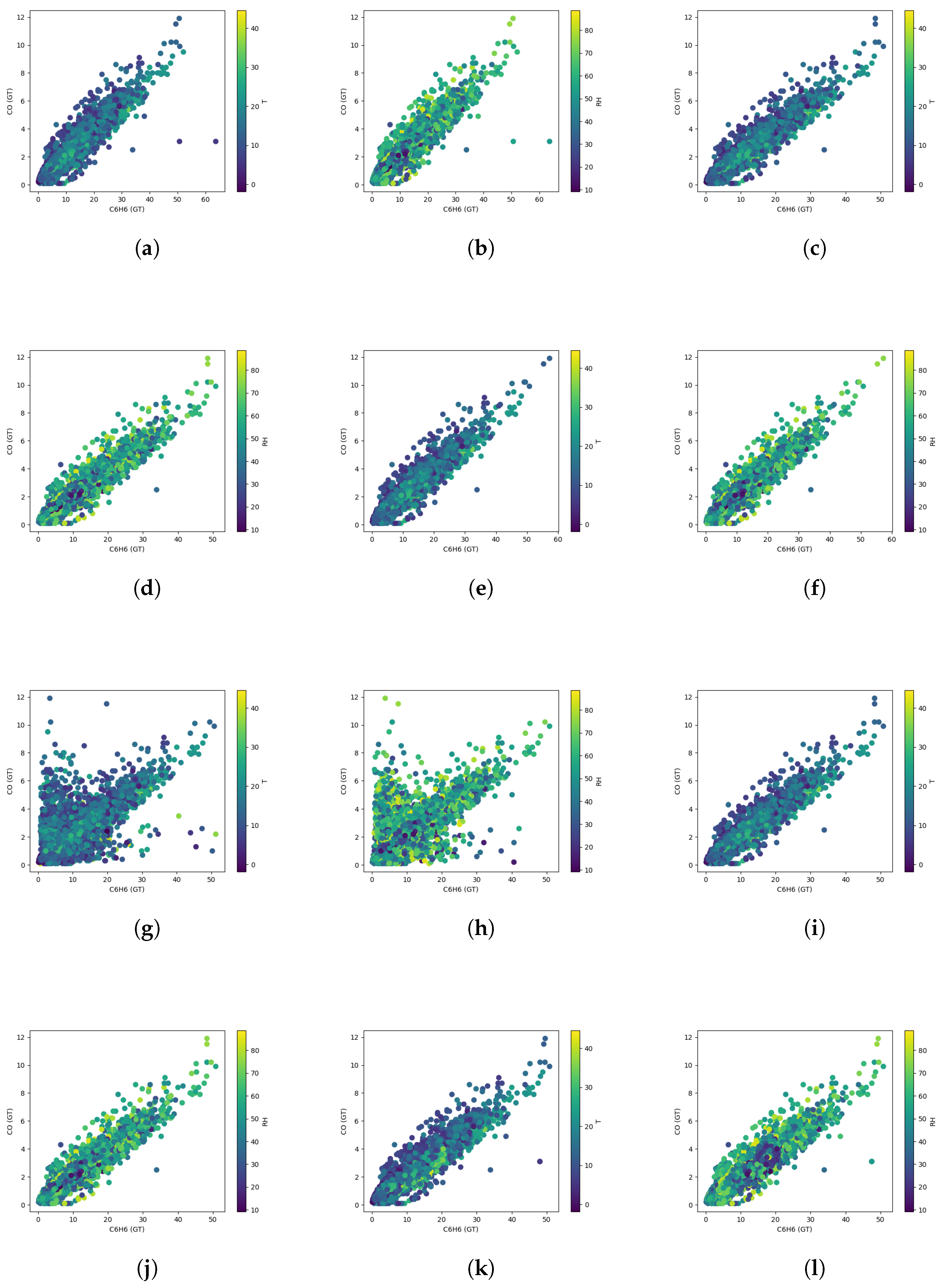
We analysed the effect of each imputation technique on the sensor calibration and compared the results to the calibration result of each imputation method.

Specifically, we introduced missing values based on the patterns listed below and evaluated the accuracy of the imputation methods based on the different scenarios:

(a)

We simulated missingness on a single variable at random, where missing ratio r = (10%, 20%, 30% and 40%).

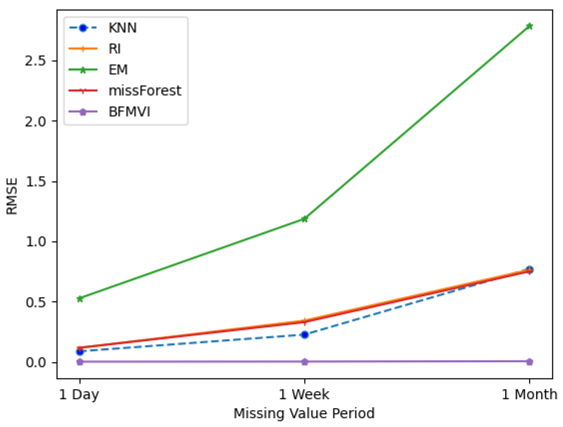
(b)

We simulated missing values on one variable, occurring over p consecutive time periods where p = (1 day, 1 week and 1 month).

A detailed description of the imputation algorithms used in our experiments can be seen in the following sections below.

4.2.1. Expectation Maximization Imputation (EMI)

This technique was proposed by [28] to handle the missing data problem. The general idea behind the EM algorithm is to iteratively estimate parameters required to predict the missing values in a given distribution by calculating the mean and variance between parameters [26]. The application of the EM algorithm usually aims at solving missing data problems. However, research has also shown the use of this algorithm in solving complex problems for complete data sets. For example, multilevel linear models, structural equation model and finite mixture [36,37,38,39].

The EM algorithm constitutes iterative processes built on two steps: the expectation step ("E-step") and maximization step ("M-step"). The initial values available in a system are required to initiate the estimation process. The E-step begins with the construction of a linear regression model, using the co-variance matrix and initial mean vector to produce estimates for missing values based on the values from the observed data. The M-step follows after the E-step and produces new parameter values for the data that have been estimated. The algorithm saves the last co-variance matrix and mean vector to determine the next E-step and builds a new regression model from the results which is then used to determine new estimates for missing values. The M-step will subsequently run again to determine new parameters from the updated estimates. The EM algorithm will iterate these two steps until the values of the co-variance matrix and mean vector no longer changes or converges, where the converged value corresponds to that of the value of the maximum likelihood estimates. The number of iterations in the EM algorithm is dependent on the number of missing values in the dataset [40,41]. Research conducted by [28] shows a detailed description of the EMI algorithm.

4.2.2. K-Nearest Neighbour (KNN) Imputation

We also employed the KNN algorithm in this study. The KNN method is a machine learning algorithm which approaches imputation by classifying the k closest observed values to missing values and using the average of these k nearest neighbours to impute missing values going by the distance measure between points [42]. Various distance factors have been applied to the KNN algorithm in research but for the purpose of this study, we used the Euclidean distance factor which is the most widely used measure that maximizes efficiency and productivity of the algorithm [43,44]. The nearest neighbours to the missing data points were determined by calculating the distance factor between the missing data point (x) as well as the observed neighbour (y), as shown in Equation (1) below.

$$Dis{t}_{xy}=\sqrt{\sum _{k=1}^m{(X_i-Y_i)}^2}$$

(1)

4.2.3. MissForest

MissForest is another iterative technique based on the Random Forest (RF) algorithm. Previous research has shown the efficiency of this algorithm in handling multivariate missing values in high dimensional datasets in a computationally efficient manner [17]. To impute missing values, the algorithm first trained the RF on the observed data using an iterative imputation scheme, after which the missing values were imputed iteratively. Section 4.3.2 provides a detailed description of the missForest technique, which is the foundation of our proposed approach.

4.2.4. Regression Imputation

Inspired by the research in [44], we also performed missing data imputation based on the traditional simple linear regression model. Generally, we generated a regression model using the variables that presented high correlation results with the imputation variable based on Equation (2) below. These variables were used to predict and replace the missing values on the target variable.

$$\widehat{Y}=a+b_1{x}_1+\dots +b_q{x}_{q,i}$$

(2)

where $\widehat{Y}$ is the dependent variable with missing values, $x_1$ is the independent variable and $b_1$ represents unknown parameters.

4.3. Our Approach

We propose an imputation model based on k-Means algorithm that is capable of choosing the most optimal imputation method. Three stages are considered in our imputation model; firstly, we partition the incomplete data into different groups based on the k-means algorithm. Secondly, missing values in each independent cluster is estimated based on the the observed values within each group. In the third stage, the algorithm selects the most suitable imputation technique for each group based on predefined imputation techniques fitted in the model.

In the next sections, we present the stages involved in the proposed imputation approach, but we first introduce some relevant notations and definitions related to the univariate missing data:

Definition 1.

A univariate data series X shows a sequence of real numbers X = $x_1,x_2,\dots ,x_n$ where N represents the length of the series.

Definition 2.

A missing sequence $V_{i,l}\in$ X is a set of continuous missing data NA where the length l ranges from i to i + l.

4.3.1. Stage 1: Partitioning the Dataset

Before grouping the data, we first of all pre-imputed missing values using distinct values, after which the dataset was split into k = 3 distinct groups. According to [45], more accurate imputation estimates could be derived when similar records are used to estimate missing instances. However, [46] argued that current clustering algorithms do not perform optimally in the presence of missing data as missing values constitute major uncertainties in a dataset, therefore affecting the usability and accuracy of existing clustering algorithms. The strategy for clustering the dataset is integrated in Algorithm 1.

4.3.2. Stage 2: Defining the Imputation Strategy

The second stage is initiated after the dataset has been group into clusters with similar records. We trained a random forest model on each group before aggregating the data. This ensured that strong predictors $X_s=1,\cdots ,p$ were used in the training process.

In our approach, we assume an n × p-dimensional matrix where X = $(X_1,\cdots ,X_n)$. We first of all use the RF algorithm to fill in missing observations in each partition created by the k-Means algorithm. A built-in routine is added to the RF algorithm for handling missing values by considering the frequency of values in the recorded variables with their RF proximities after initially training the model on the dataset pre-imputed with mean values [47]. This approach mostly requires a fully observed response variable before the RF model can be trained. However, we directly estimated the missing values by using the RF model on a training set containing only the observed data, with X, being the matrix with complete data and $X_s$ representing the sample with missing vales $i_{miss}^{\left(s\right)}\subseteq \{1,\cdots ,n\}$. To better understand the training process, we separate the data into four parts as described below:

• $y_{obs}^{\left(s\right)}\to$ representing the values that are present in the variable $X_s$
• $y_{miss}^{\left(s\right)}\to$ representing the values that are missing in the variable $X_s$
• $x_{obs}^{\left(s\right)}\to$ representing the observations, $i_{obs}^{\left(s\right)}$ = {1,…,n}\$i_{miss}^{\left(s\right)}$ of the predictor variable in $X_s$
• $x_{miss}^{\left(s\right)}\to$ representing the observations, $i_{miss}^{\left(s\right)}$ of the predictor variable in $X_s$

It is important to note that $i_{obs}^{\left(s\right)}$ points only to the observed values in $X_s$. Therefore, $x_{obs}^{\left(s\right)}$ is not completely observed and likewise, $x_{miss}^{\left(s\right)}$ is not completely missing.

Similar to the work in [17], the process is initiated by pre-imputing the missing values in X with the mean of the distribution or any imputation method, after which the predictors $X_s=1,\cdots ,p$ are stacked in ascending order considering the amount of values that are missing. Each missing value in $X_s$ is then imputed by first of all fitting the RF on the response $y_{obs}^{\left(s\right)}$ and predictor variable $x_{obs}^{\left(s\right)}$. Next, the trained RF model is applied to $x_{miss}^{\left(s\right)}$ to predict the missing values of $y_{miss}^{\left(s\right)}$. The imputation process is repeated until the set stopping criterion ($\gamma$) has been met. This is achieved when the difference between the most recent imputed data matrix and the old matrix has an increase for the first time, considering the variable types present. In our approach, we take the $n\times p$ matrix to be a set of set of continuous variables. Therefore, the difference in the new and previous imputed matrix N is defined as:

$${\Delta }_N=\frac{{\sum }_{j\in N}{(X_{new}^{imp}-X_{old}^{imp})}^2}{{\sum }_{j\in N}{(X_{new}^{imp})}^2}$$

(3)

This step is followed by two additional imputation phases where missing values in each cluster is also estimated using a kNN and linear regression model.

Still considering an $n\times p$ matrix $X_s$, the procedure for next imputation phase is described as follows;

• The missing values in each cluster matrix $C_i$ are located.
• The kNN vectors are defined by; $x_{\left(1\right)}^D,\dots ,x_n^D$ with $d(x_{i,}{x}_{\left(1\right)})\le ,\dots ,\le d(x_{i,}{x}_{\left(k\right)})$, where $x_{\left(1\right)}^D$ represents the rows of the matrix $X^D$, and $d(x_{i,}{x}_{\left(k\right)})$ is the distance given by Equation (1).
• For each point $\left(y\right)$ in $C_i$, the distance (x, y) between the missing point and nearest imputed value is stored in a similarity array $\left(S\right)$.
• The array $\left(S\right)$ is sorted in descending order and the top K data for $\left(y\right)$ in $C_i$ is selected for imputation.

The linear regression imputation process follows, as described below;

• For each matrix $C_i$ the data was split into four parts similar to the RF method where a regression model was trained on the response $y_{obs}^{\left(s\right)}$ and predictor variable $x_{obs}^{\left(s\right)}$.
• The trained regression model is then used to predict the missing values in $X_s$.

4.3.3. Step 3: Selecting the Best Fit Estimation

After computing the missing values, the next stage is the selection of the most suitable imputation method within each group. For each data matrix $C_i$, we make our selection by estimating the error between the previous imputation $y_{pre,i}$ and current imputation $y_{cur,i}$ based on the equation below;

$$err=\sqrt{\frac{1}{n}\sum _{i=1}^n{y}_{pre,i}-y_{cur,i}}$$

(4)

we set the result of the RF imputation as our threshold $\gamma$ and place $y_{pre,i}$≡$\gamma$ as the initial value of the previous estimate as described in Algorithm 1.

Lastly, we use a reverse error score function RES(r) to obtain the final imputation sequence. This is based on two RMSE calculations between the previous imputation estimate with the lowest error and our given threshold $\gamma$ . A sequence that gives the lowest error score is chosen as the optimal imputation estimate for the given distribution.

Definition 3.

A reverse error score function RES(r) representing the error between γ and the final sequence ${\beta }_{Ci}$ in each group $C_i$ is expressed as:

$$M_{\gamma }=\frac{\partial \left(\gamma \right)}{{\partial }_n}=\sqrt{\frac{{\sum }_{i=1}^N{(X_{\gamma }-{\widehat{y}}_{{\beta }_{ci}})}^2}{n}}$$

(5)

$$M_{{\beta }_{ci}}=\frac{\partial \left({\beta }_{ci}\right)}{{\partial }_n}=\sqrt{\frac{{\sum }_{i=1}^N{({\widehat{y}}_{{\beta }_{ci}}-X_{\gamma })}^2}{n}}$$

(6)

$$RES\left(r\right)=M(\gamma ,{\beta }_{ci})=\left[\frac{\partial \left(\gamma \right)}{{\partial }_n}\frac{\partial \left({\beta }_{ci}\right)}{{\partial }_n}\right]$$

(7)

where γ is the imputation threshold for $C_i$ and ${\beta }_{Ci}$ is the best estimate from the previously chosen imputation techniques.

Algorithm 1k-Best Fit Estimation Model.

Input: Incomplete matrix X (n x p). Parameter: $\gamma$, missing value: vs. Output: Dataset with Imputed values $X_s$. 1: Pre-impute missing values in matrix X (n x p) with distinct single imputation values 2: Select initial centers k at random C = {$c_1$,…,$c_k$} 3: whileconvergence criteria is not metdo 4:     assignment step: 5:     for i = 1,…,N do 6:         locate nearest centroid $c_k$∈C to points {$p_i,\cdots ,p_n$} 7:         append points {$p_i,\cdots ,p_n$} to the set $C_k$ centroid 8:         Update: 9:         for i = 1,…,k do 10:            $c_i$→ center of all points in $C_i$ 11:         end for 12:     end for 13: end while 14: Assign cluster label ($C_{ik}$) to points {$p_1,\cdots ,p_n$} ∈ X 15: while 1 do 16:     for each v ∈$C_i$ do 17:         $R{F}_i^1$ = missForest ($p_i$∈$C_i$) 18:         $R{I}_i^1$ = regression ($p_i$∈$C_i$) 19:         $kN{N}_i^1$ = k-Nearest Neighbour ($p_i$∈$C_i$) 20:     end for 21:     $er{r}_{ci}=\sqrt{\frac{1}{n}{\sum }_{i=1}^n{\gamma }_{pre,i}-{\alpha }_{cur,i}}$ 22:     if $R{I}_{err}\le$$kN{N}_{err}$ then 23:         $R{I}_i^1\to {\beta }_{Ci}$ 24:     else $kN{N}_i^1\to {\beta }_{Ci}$ // Store imputed value in a temporary array 25:     end if 26:     Get the imputation sequence ($M_{}^{{}^{\prime }}$) and compute a reverse error score function RES(r): 27:     for $v=1:k$ do 28:         Get the reverse error score RES(r) using Equation (7) 29:         if ${\beta }_{Ci,err}$ ≤ ${\gamma }_{err}$ then 30:            ${\beta }_{Ci}$↦$C_i$ 31:         else $\gamma$↦$C_i$ 32:         end if 33:     end for 34: end while 35: Return imputed dataset $X_s$;

4.4. Model Evaluation

In this section, the accuracy of the imputation and calibration models was first evaluated and compared with the estimated values and calibrated sensor responses to the measurements derived from the original sensor data using the following error metrics: Root Mean Squared Error (RMSE), Mean Absolute Error (MAE) and Coefficient of Determination ($R^2$).

$$RMSE=\sqrt{\frac{1}{N}}\sum _{i=1}^N{(Y_i-{\widehat{y}}_i)}^2$$

(8)

$$MAE=\frac{1}{N}\sum _{i=1}^N\left(\right|Y_i-{\widehat{y}}_i\left|\right)$$

(9)

where N represents the sample size, $Y_i$ is the original data matrix and ${\widehat{y}}_i$ is the imputed data.

A low RMSE and MAE shows better model performance and the closer the $R^2$ value is to 1, the better the model performance. The performance of each imputation method was evaluated and used to build the calibration models.

5. Results

We present the results of our analysis in the following subsections. Evaluated the performance of each imputation technique and their effect on sensor calibration.

5.1. Imputation

We compared the accuracy of the different imputation techniques. First, we simulated artificial missing values on the $C_6{H}_6$ sensor variable at different rates {10%, 20%, 30%, 40%}. The different techniques (kNN, RI, missForest, EM and BFMVI) were used to impute the missing values and the accuracy of these techniques at the different missing data rates were calculated.

Table 1. Performance and computational complexity of imputation techniques.

Imputation Method	Avg. Computational Complexity (s)	Missing Rate	RMSE	${\mathit{R}}^2$	MAE
KNN	0.82	10%	0.941595	0.984187	0.216405
		20%	1.410407	0.964461	0.452831
		30%	1.831899	0.964461	0.694035
		40%	1.930442	0.933555	0.861461
RI	0.85	10%	0.802989	0.98831	0.193356
		20%	1.206893	0.97327	0.392866
		30%	1.630087	0.949827	0.61114
		40%	1.722670	0.943538	0.771931
EM	2.28	10%	3.083324	0.824947	0.719108
		20%	4.507154	0.608994	1.435791
		30%	5.445520	0.405416	2.189204
		40%	6.398958	0.152979	2.914241
missForest	1.71	10%	0.835237	0.987369	0.197484
		20%	1.231309	0.972118	0.392628
		30%	1.631028	0.949937	0.60595
		40%	1.746202	0.941935	0.77397
BFMVI	3.39	10%	0.011758	0.999998	0.000599
		20%	0.029012	0.999985	0.001917
		30%	0.215160	0.999165	0.006739
		40%	0.169418	0.999483	0.006136

shows the performance of the different techniques. From the results, our approach recorded the best imputation accuracy across the different rates of missing data. This could be explained by the use of strong predictors through clustering the data before imputation was carried out. The results of the RF and RI imputation methods also showed similar imputation performance, owing to the effect of the auxiliary variables (i.e., CO, NMHC, NO_x and O₃) that showed strong correlation with the missing sensor variable and were added to the imputation model.

We also assessed the performance of the imputation techniques on missing data occurring over a consecutive period of time {1 day, 1 week and 1 month} as seen in

Table 2. Comparison of Imputation Techniques on $C_6{H}_6$ Missing Values occurring over Consecutive Periods.

Missing Period	KNN	RI	EM	missForest	BFMVI
1 Day	0.0872	0.115932	0.526072	0.11624	0.001016
1 Week	0.225566	0.341941	1.185411	0.328895	0.002169
1 Month	0.770596	0.763162	2.785029	0.750043	0.005263

and Figure 3. In general, across all imputation tasks examined in this paper, BFMVI illustrates a reliable performance in handling the different rates and characteristics of missing data considered in this study as opposed to the other imputation techniques.

The average computational complexity $T_{avg}\left(n\right)$ of the imputation techniques were also computed based on the function $T\left(n\right)=cn$ where T represents the time, n represents the input size and c represents some constant [48]. We computed the complexity of the imputation techniques on each missing data rate (10–40%) and obtained the average complexity based on $T_{avg}\left(n\right)$ = $T\left(n\right)/m$, where m = 4 simulations. Overall, KNN imputation showed the best computational performance among all other imputation techniques considered with an averege of 0.82. Our proposed BFMVI technique however showed a trade-off between accuracy and complexity with a higher average computational complexity of 3.39 owing to the imputation process which computes multiple imputation options for the final process.

5.2. Sensor Calibration

After missing values were imputed using different techniques, we investigated the effect of each imputation technique for the purpose of sensor calibration. Sensor calibration commonly require complete observations of the reference and sensor measurement. Therefore, the use of efficient imputation strategies is paramount.

Different supervised machine learning techniques were employed to calibrate the sensor data (MLR, DT and RF). To assess the effect of the imputation techniques on the calibration process, we conducted our analysis using the results of the imputed data at 30% missing rate. Calibrating sensor data using the BFMVI data showed stronger results when contrasted with the original data. The results in

Table 3. Comparison of Imputation Techniques on $C_6{H}_6$ Sensor Calibration.

Imputation Method	Performance Measure	MLR	DT	RF
Original Data	RMSE	1.105198	2.675627	1.307132
	R${}^2$	0.977588	0.852582	0.967482
	MAE	0.782843	1.924280	0.941910
KNN	RMSE	0.921755	1.831899	1.443856
	R${}^2$	0.983985	0.939847	0.961877
	MAE	0.711107	0.694035	0.703279
RI	RMSE	0.85446	1.630087	1.28414
	R${}^2$	0.985646	0.949827	0.968328
	MAE	0.656718	0.61114	0.622812
EM	RMSE	2.529208	5.450468	4.118277
	R${}^2$	0.757888	0.403799	0.530481
	MAE	1.928332	2.196589	2.132884
MissForest	RMSE	0.823423	1.631028	1.287602
	R${}^2$	0.986708	0.949937	0.968244
	MAE	0.634978	0.60595	0.61483
BFMVI	RMSE	0.031015	0.201528	0.195777
	R${}^2$	0.999982	0.999268	0.999308
	MAE	0.023258	0.006227	0.010485

shows the calibration results of the different imputation methods on the $C_6{H}_6$ sensor. Figure 4 also shows the response of some meteorological factors on the imputation techniques. On each calibration method, the result of the BFMVI imputed data showed more accurate results. The RI, missForest and kNN methods also showed good performance with $R^2$ score > 0.9 for all calibration processes. Calibrating the the sensor with the MLR model trained on the BFMVI imputed data showed the best performance with an RMSE score of 0.031. Overall, calibrating the sensor on the filtered CCA data showed promising results. However, there was a noticeable reduction in error from the calibration on the imputed data compared to the original CCA data.

6. Conclusions and Future Work

In this work, we explored various missing value imputation strategies for LCS deployed to generate data for air quality monitoring stations. We investigated imputation techniques such as kNN, RI, EM, missForest and proposed the BFMVI technique for handling missing data. In this study, the BFMVI technique shows the most promising performance for estimating univariate missing data when compared with other imputation techniques. From our analysis, the concentrations of other auxiliary sensor variables such as CO, NMHC, NO_x and O₃ exhibiting strong correlation with the target variable C₆H₆ were added to the imputation model, which had strong effects on the predictions, while it is unfeasible to evaluate the accuracy of imputation techniques when the true values are not known, the authors took the fully observed dataset and introduced artificial missing values using two patterns to test the accuracy of the imputation methods. Overall, our proposed BFMVI method showed promising results when compared to the other competing algorithms when applied to a real world Air Quality monitoring dataset. Furthermore, we took the dataset imputed at 30% for all the imputation techniques and evaluated their effect on the sensor calibration process. The authors evaluated the efficiency of various calibration models (DT, MLR, and RF) when trained on various imputed datasets. Results showed improvements when the MLR model was trained on our proposed BFMVI approach with an RMSE of 0.0310 as opposed to other techniques.

Due to time constraint, this study could not consider other gas/electrochemical sensor data with multivariate missing values. Future research could concentrate on other types of gas sensor data, including Non-Dispersive Infrared (NDIR) sensor data.

References

1. Lee, G.H.; Han, J.; Choi, J.K. MPdist-based missing data imputation for supporting big data analyses in IoT-based applications. Future Gener. Comput. Syst. 2021, 125, 421–432. [Google Scholar] [CrossRef]
2. Al-Aqrabi, H.; Johnson, A.P.; Hill, R.; Lane, P.; Alsboui, T. Hardware-intrinsic multi-layer security: A new frontier for 5G enabled IIoT. Sensors 2020, 20, 1963. [Google Scholar] [CrossRef] [PubMed] [Green Version]
3. Al-Aqrabi, H.; Liu, L.; Hill, R.; Antonopoulos, N. A multi-layer hierarchical inter-cloud connectivity model for sequential packet inspection of tenant sessions accessing BI as a service. In Proceedings of the 2014 IEEE International Conference on High Performance Computing and Communications, 2014 IEEE 6th International Symposium on Cyberspace Safety and Security, 2014 IEEE 11th International Conference on Embedded Software and System (HPCC, CSS, ICESS), Paris, France, 20–22 August 2014; pp. 498–505. [Google Scholar]
4. Al-Aqrabi, H.; Hill, R.; Lane, P.; Aagela, H. Securing manufacturing intelligence for the industrial internet of things. In Proceedings of the Fourth International Congress on Information and Communication Technology, Singapore, 22 January 2019; pp. 267–282. [Google Scholar]
5. De Vito, S.; Massera, E.; Piga, M.; Martinotto, L.; Di Francia, G. On field calibration of an electronic nose for benzene estimation in an urban pollution monitoring scenario. Sens. Actuators B Chem. 2008, 129, 750–757. [Google Scholar] [CrossRef]
6. Mazzeo, N.A.; Venegas, L.E. Evaluation of turbulence from traffic using experimental data obtained in a street canyon. Int. J. Environ. Pollut. 2005, 25, 164–176. [Google Scholar] [CrossRef]
7. Loy-Benitez, J.; Heo, S.; Yoo, C. Imputing missing indoor air quality data via variational convolutional autoencoders: Implications for ventilation management of subway metro systems. Build. Environ. 2020, 182, 107135. [Google Scholar] [CrossRef]
8. Chen, Y.; Lv, Y.; Wang, F.Y. Traffic flow imputation using parallel data and generative adversarial networks. IEEE Trans. Intell. Transp. Syst. 2019, 21, 1624–1630. [Google Scholar] [CrossRef]
9. Sanjar, K.; Bekhzod, O.; Kim, J.; Paul, A.; Kim, J. Missing data imputation for geolocation-based price prediction using KNN–mcf method. ISPRS Int. J. Geo-Inf. 2020, 9, 227. [Google Scholar] [CrossRef] [Green Version]
10. Wells, B.J.; Chagin, K.M.; Nowacki, A.S.; Kattan, M.W. Strategies for handling missing data in electronic health record derived data. Egems 2013, 1, 1035. [Google Scholar] [CrossRef]
11. Ehrlinger, L.; Grubinger, T.; Varga, B.; Pichler, M.; Natschläger, T.; Zeindl, J. Treating missing data in industrial data analytics. In Proceedings of the 2018 Thirteenth International Conference on Digital Information Management (ICDIM), Berlin, Germany, 24–26 September 2018; IEEE: Piscataway, NJ, USA; pp. 148–155. [Google Scholar]
12. Read, S.H. Applying Missing Data Methods to Routine Data Using the Example of a Population-Based Register of Patients with Diabetes. Ph.D. Thesis, University of Edinburgh, Edinburgh, UK, 4 July 2015. [Google Scholar]
13. Osman, M.S.; Abu-Mahfouz, A.M.; Page, P.R. A survey on data imputation techniques: Water distribution system as a use case. IEEE Access 2018, 6, 63279–63291. [Google Scholar] [CrossRef]
14. Graham, J.W. Missing data analysis: Making it work in the real world. Annu. Rev. Psychol. 2009, 60, 549–576. [Google Scholar] [CrossRef] [Green Version]
15. Azur, M.J.; Stuart, E.A.; Frangakis, C.; Leaf, P.J. Multiple imputation by chained equations: What is it and how does it work? Int. J. Methods Psychiatr. Res. 2011, 20, 40–49. [Google Scholar] [CrossRef] [PubMed]
16. Chen, X.; He, Z.; Sun, L. A Bayesian tensor decomposition approach for spatiotemporal traffic data imputation. Transp. Res. Part C Emerg. Technol. 2019, 98, 73–84. [Google Scholar] [CrossRef]
17. Stekhoven, D.J.; Bühlmann, P. MissForest—non-parametric missing value imputation for mixed-type data. Bioinformatics 2012, 28, 112–118. [Google Scholar] [CrossRef] [PubMed] [Green Version]
18. Mesquita, D.P.; Gomes, J.P.P.; Rodrigues, L.R. Artificial neural networks with random weights for incomplete datasets. Neural Process. Lett. 2019, 50, 2345–2372. [Google Scholar] [CrossRef]
19. Snow, D. MTSS-GAN: Multivariate Time Series Simulation Generative Adversarial Networks. Available online: https://papers.ssrn.com/sol3/papers.cfm?abstract_id=3616557 (accessed on 2 May 2022).
20. Xie, R.; Jan, N.M.; Hao, K.; Chen, L.; Huang, B. Supervised variational autoencoders for soft sensor modeling with missing data. IEEE Trans. Ind. Inf. 2019, 16, 2820–2828. [Google Scholar] [CrossRef]
21. Peralta, M.; Jannin, P.; Haegelen, C.; Baxter, J.S. Data imputation and compression for Parkinson’s disease clinical questionnaires. Artif. Intell. Med. 2021, 114, 102051. [Google Scholar] [CrossRef]
22. Bowman, S.R.; Vilnis, L.; Vinyals, O.; Dai, A.M.; Jozefowicz, R.; Bengio, S. Generating sentences from a continuous space. arXiv 2015, arXiv:1511.06349. [Google Scholar]
23. Agbo, B.; Qin, Y.; Hill, R. Best Fit Missing Value Imputation (BFMVI) Algorithm for Incomplete Data in the Internet of Things. In Proceedings of the 5th International Conference on Internet of Things, Big Data and Security (IoTBDS 2020), Prague, Czech Republic, 7–9 May 2020; pp. 130–137. Available online: https://www.scitepress.org/Papers/2020/95782/95782.pdf (accessed on 4 April 2022).
24. Okafor, N. Missing Data Imputation on IoT Data Networks: Implications for On-site Sensor Calibration. IEEE Sens. J. 2021, 21, 22833–22845. [Google Scholar] [CrossRef]
25. Little, R.J.; Rubin, D.B. Statistical Analysis with Missing Data; John Wiley & Sons: Hoboken, NJ, USA, 2019; Available online: https://www.wiley.com/en-us/Statistical+Analysis+with+Missing+Data%2C+3rd+Edition-p-9780470526798 (accessed on 4 April 2022).
26. Bashir, F. Handling of Missing Values in Static and Dynamic Data Sets. PhD Thesis, University of Sheffield, Sheffield, UK, 2019. Available online: https://etheses.whiterose.ac.uk/23283/ (accessed on 4 April 2022).
27. Alsaber, A.R.; Pan, J.; Al-Hurban, A. Handling complex missing data using random forest approach for an air quality monitoring dataset: A case study of Kuwait environmental data (2012 to 2018). Int. J. Environ. Res. Public Health 2021, 18, 1333. [Google Scholar] [CrossRef]
28. Dempster, A.P.; Laird, N.M.; Rubin, D.B. Maximum likelihood from incomplete data via the EM algorithm. J. R. Stat. Soc. Ser. B (Methodol.) 1977, 39, 1–22. [Google Scholar]
29. Zhang, L.; Pan, H.; Wang, B.; Zhang, L.; Fu, Z. Interval Fuzzy C-means Approach for Incomplete Data Clustering Based on Neural Networks. J. Internet Technol. 2018, 19, 1089–1098. [Google Scholar]
30. Gupta, A.; Lam, M.S. Estimating missing values using neural networks. J. Oper. Res. Soc. 1996, 47, 229–238. [Google Scholar] [CrossRef]
31. Ravi, V.; Krishna, M. A new online data imputation method based on general regression auto associative neural network. Neurocomputing 2014, 138, 106–113. [Google Scholar] [CrossRef]
32. Guastella, D.A.; Marcillaud, G.; Valenti, C. Edge-based missing data imputation in large-scale environments. Information 2021, 12, 195. [Google Scholar] [CrossRef]
33. Spinelle, L.; Gerboles, M.; Villani, M.G.; Aleixandre, M.; Bonavitacola, F. Field calibration of a cluster of low-cost available sensors for air quality monitoring. Part A: Ozone and nitrogen dioxide. Sens. Actuators B Chem. 2015, 215, 249–257. [Google Scholar] [CrossRef]
34. UCI Air Quality Data Set. Available online: https://archive.ics.uci.edu/ml/datasets/air+quality (accessed on 2 February 2022).
35. Phan, T.-T.-H.; Caillault, É.P.; Lefebvre, A.; Bigand, A. Dynamic time warping-based imputation for univariate time series data. Pattern Recognit. Lett. 2020, 139, 139–147. [Google Scholar]
36. Liang, J.; Bentler, P.M. An EM algorithm for fitting two-level structural equation models. Psychometrika 2004, 69, 101–122. [Google Scholar] [CrossRef]
37. Muthén, B.; Shedden, K. Finite mixture modeling with mixture outcomes using the EM algorithm. Biometrics 1999, 55, 463–469. [Google Scholar] [CrossRef]
38. Neale, M.C.; Boker, S.M.; Xie, G.; Maes, H.M. Statistical Modeling; Department of Psychiatry, Virginia Commonwealth University: Richmond, VA, USA, 1999; Available online: http://ftp.vcu.edu/pub/mx/doc/mxmang10.pdf (accessed on 4 April 2022).
39. Raudenbush, S.W.; Bryk, A.S. Hierarchical Linear Models: Applications and Data Analysis Methods; SAGE: Newbury Park, CA, USA, 2002; Available online: https://us.sagepub.com/en-us/nam/hierarchical-linear-models/book9230 (accessed on 4 April 2022).
40. Neal, R.M.; Hinton, G.E. A view of the EM algorithm that justifies incremental, sparse, and other variants. In Learning in Graphical Models; Springer: Dordrecht, The Netherlands, 1998; pp. 355–368. Available online: https://link.springer.com/chapter/10.1007/978-94-011-5014-9_12 (accessed on 4 April 2022).
41. Bilmes, J.A. A gentle tutorial of the EM algorithm and its application to parameter estimation for Gaussian mixture and hidden Markov models. Int. Comput. Sci. Inst. 1998, 4, 126. [Google Scholar]
42. Maillo, J.; Ramírez, S.; Triguero, I.; Herrera, F. kNN-IS: An Iterative Spark-based design of the k-Nearest Neighbors classifier for big data. Knowl. Based Syst. 2017, 117, 3–15. [Google Scholar] [CrossRef] [Green Version]
43. Amirteimoori, A.; Kordrostami, S. A Euclidean distance-based measure of efficiency in data envelopment analysis. Optimization 2010, 59, 985–996. [Google Scholar] [CrossRef]
44. Emmanuel, T.; Maupong, T.; Mpoeleng, D.; Semong, T.; Banyatsang, M.; Tabona, O. A Survey On Missing Data in Machine Learning. J. Big Data 2021, 8, 1–37. [Google Scholar] [CrossRef] [PubMed]
45. Zhang, Q.; Yang, L.T.; Chen, Z.; Xia, F. A High-Order Possibilistic C-Means Algorithm for Clustering Incomplete Multimedia Data. IEEE Syst. J. 2015, 11, 2160–2169. [Google Scholar] [CrossRef]
46. Zhao, L.; Chen, Z.; Yang, Z.; Hu, Y.; Obaidat, M.S. Local similarity imputation based on fast clustering for incomplete data in cyber-physical systems. IEEE Syst. J. 2018, 12, 1610–1620. [Google Scholar] [CrossRef]
47. Breiman, L. Random Forests. Mach. Learn. 2001, 45, 5–32. [Google Scholar] [CrossRef] [Green Version]
48. Maresca, P. The Running Time of an Algorithm. Ser. Softw. Eng. Knowl. Eng. 2003, 13, 17–32. [Google Scholar] [CrossRef]
Figure 1. Pattern of missing value occurrence.
Futureinternet 14 00143 g001
Figure 2. Correlation coefficients of air quality sensors.
Futureinternet 14 00143 g002
Figure 3. Comparison of Imputation Techniques on C 6 H 6 Missing Values occurring over Consecutive Periods.
Futureinternet 14 00143 g003
Figure 4. Scatter plot showing the effect of various imputation techniques on the sensor data color-coded with Temperature (T) and Relative Humidity (RH) meteorological factors: (a,b) Original data, (c,d) kNN Imputation, (e,f) Regression Imputation, (g,h) EM Imputation, (i,j) missForest Imputation and (k,l) BFMVI.
Futureinternet 14 00143 g004