Clinical Trial Classification of SNS24 Calls with Neural Networks

Abstract

SNS24, the Portuguese National Health Contact Center, is a telephone and digital public service that provides clinical services. SNS24 plays an important role in the identification of users’ clinical situations according to their symptoms. Currently, there are a number of possible clinical algorithms defined, and selecting the appropriate clinical algorithm is very important in each telephone triage episode. Decreasing the duration of the phone calls and allowing a faster interaction between citizens and SNS24 service can further improve the performance of the telephone triage service. In this paper, we present a study using deep learning approaches to build classification models, aiming to support the nurses with the clinical algorithm’s choice. Three different deep learning architectures, namely convolutional neural network (CNN), recurrent neural network (RNN), and transformers-based approaches are applied across a total number of 269,654 call records belonging to 51 classes. The CNN, RNN, and transformers-based model each achieve an accuracy of 76.56%, 75.88%, and 78.15% over the test set in the preliminary experiments. Models using the transformers-based architecture are further fine-tuned, achieving an accuracy of 79.67% with Adam and 79.72% with SGD after learning rate fine-tuning; an accuracy of 79.96% with Adam and 79.76% with SGD after epochs fine-tuning; an accuracy of 80.57% with Adam after the batch size fine-tuning. Analysis of similar clinical symptoms is carried out using the fine-tuned neural network model. Comparisons are done over the labels predicted by the neural network model, the support vector machines model, and the original labels from SNS24. These results suggest that using deep learning is an effective and promising approach to aid the clinical triage of the SNS24 phone call services.

1. Introduction

SNS24, the Portuguese National Health Contact Center, is a national telephone and digital public service in Portugal. SNS24 allows citizens access facility, guarantees equity, and simplifies access to the National Health System (SNS). SNS24 provides clinical services for the citizens, such as triage, counseling, referral, and non-clinical help. These services are essential to the public health and safety. Health professionals and specifically nurses with distinct training supplied by SNS24 provide the telephone clinical services.

Currently, 59 possible clinical algorithms are developed by health professionals and approved by the Directorate General of Health (DGS). Following the pre-defined clinical pathways, the health professional or nurse selects the most appropriate one according to the citizen’s self-reported symptoms and relevant information about medical history. The selection of the clinical algorithms leads to five possible final referrals: self-care, clinical assessment at a primary health care center, clinical assessment in hospital emergency, transference to the National Medical Emergency Institute (INEM), or transference to the Poison Information Center. All the 59 clinical pathways start by asking screening questions, aiming to identify critical situations which need immediate health care and that are rapidly transferred to National Medical Emergency Institute. For non-emergencies, nurses must ensure that the main symptoms reported by the citizen are correctly mapped to allow the choice of the clinical pathway. Age, gender, and clinical history should also be considered during this process since this information is often crucial to the selection of the most appropriate clinical pathway. The choice of the clinical pathway by the health care professionals in each telephone triage episode is extremely important since it will determine the final referral. These pathways use a risk-averse system of prioritization, as other triage protocols such as the Manchester Triage System [1]. For this reason, SNS24 has an important role in the identification of users’ clinical situation and the correct referral to health services according to their symptoms.

This work explores using neural network (NN) architectures to build classification models for SNS24 clinical triage, aiming to improve the quality and performance of telephone triage service; support the nurses in the triage process, particularly with clinical algorithm’s choice; decrease the duration of the phone calls and allow a finer and faster interaction between citizens and SNS24 service. The main contributions of this paper are summarized as follows:

• Three deep learning (DL) based classification architectures are compared, namely CNN (convolutional neural network), RNN (recurrent neural network), and transformers-based architecture, in the automatic clinical trial classification of the SNS24 health calls.
• An empirical process for fine-tuning hyperparameters is explored. This process practically shortens the tuning time and theoretically achieves near-optimal classification accuracy.
• Comprehensive experimental results show that neural network models outperform shallow machine learning models with the testing accuracies on the same SNS24 clinical dataset.
• Useful suggestions are provided to the SNS24 health center. Practical analysis among similar clinical symptoms is carried out. Predictions from SNS24 triage, neural network models, and shallow machine learning models are compared.

The rest of the paper is organized as follows. Section 2 reviews the related work, Section 3 describes the materials used and presents the methods proposed. The experiments are demonstrated in Section 4, and the results and discussion are presented in Section 5. Section 6 analyzes similar clinical symptoms based on the built neural network models. Section 7 compares the labels predicted by the trained models with the original labels. Finally, the paper is concluded in Section 8.

2. Literature Review

Applying machine learning and deep learning technologies in healthcare domain is an active research topic [2]. A wide variety of paradigms, such as linear, probabilistic, and neural networks, has been proposed for clinical classification problems. For examples, Spiga et al. [3] used machine learning techniques for patient stratification and phenotype investigation in rare diseases; Sidey et al. [4] used machine learning techniques for cancer diagnosis. While applying traditional machine learning methods on clinical text classification, feature engineering is generally carried out using different forms of knowledge sources or rules. However, these approaches usually could not automatically learn effective features.

Recently, neural network methods which show capable feature learning ability have been successfully applied to clinical domain classification. Some works have also compared the performance between deep learning and shallow machine learning approaches and presented better performances when using the former approaches.

Research work by Shin et al. [5] shows that the overall performance of the systems can be improved using Deep Learning architectures. They used neural network models to classify radiology electronic health records. They compared two neural network classification models, CNN (convolution neural network) and NAM (neural attention mechanism), with the baseline SVM model. On average, the two neural models (CNN and NAM) achieved an accuracy of 87% and an improvement of 3% over the SVM baseline model.

Wu and Wang [6] used CNN in predicting the single underlying cause of death from a list of relevant medical conditions. They worked on a dataset containing 1,499,128 records and 1180 possible classes as causes of death. They compared the CNN models to several shallow classifiers (SVM, naïve bayes, random forest, and traditional BoW classification techniques). The CNN model achieved around 75% accuracy and was able to outperform all other shallow classifier models.

Mullenbach et al. [7] presented a convolutional neural network for multi-label document classification, aiming to predict the most relevant segments for the possible medical codes from clinical texts. They evaluated the approach on the MIMIC-II and MIMIC-III datasets, two open-access datasets of texts and structured records from the hospital ICU. Their method obtained a precision of 0.71 and a micro-F1 of 0.54 on the MIMIC-III dataset, and a precision of 0.52 and a micro-F1 of 0.44 on the MIMIC-II dataset.

Hughes et al. [8] used a CNN-based approach for sentence-level classification of medical documents into one of the 26 categories. Their results showed that when compared with the shallow learning methods, the CNN-based approach captured more complex features to represent the semantics of the sentence. The CNN-based model achieves an accuracy of 68%, the highest score among all the tested models.

Baker et al. [9] researched on using CNN models to classify biomedical texts, and the experiments were carried out on a cancer related dataset. Their evaluations showed that a basic CNN model achieved competitive performance compared with an SVM (Support Vector Machine) trained using manually optimized engineered features. The CNN-based model outperformed the SVM with modifications to the CNN hyperparameters, initialization, and training process.

Zhou et al. [10] experimented an integrated CNN-RNN model to provide patients with pre-diagnosis suggestions or clinic guidance online. Their experiments were carried out on the available online medical data. CNN, RNN, RCNN (Region CNN), CRNN (Convolutional RNN), and CNN-RNN models were compared. The integrated CNN-RNN model improved classification precision and was efficient in training efficiency.

Gao et al. [11] explored using CNN, RNN, and RCNN in clinical department recommendations. The experiments were carried out on a local constructed corpus consisting with 20 thousands patient symptom descriptions. The RCNN model showed better accuracy than when compared to CNN or RNN models, achieving an accuracy score of 76.51%.

In more recent research, transformers were compared against CNN models and hierarchical self-attention networks (HiSAN) [12]. The experimental results showed that generally, the CNN and HiSAN models achieved better performance than the BERT (Bidirectional Encoder Representations from Transformers) models.

Behera et al. [13] compared five deep learning based classification models, including DNN, RNN, CNN, RCNN, and RMDL (Random Multimodel Deep Learning), in automatic classification of four benchmark biomedical datasets. Among all deep learning models, the RMDL model provides the best classification performance on three datasets, and the RCNN classifier performs best on one dataset. Moreover, the work compared the performance between deep learning and shallow learning algorithms and showed that all the deep learning algorithms provided better classification performances.

Al-Garadi et al. [14] explored using text classification approaches for the automatic detection of non-medical prescription medication usage. Their work compared transformers-based language models, fusion-based approaches, several traditional machine learning and deep learning approaches. The results showed that the BERT and fusion-based models outperformed the others using machine learning and other deep learning techniques.

Mascio et al. [15] explored using several word representations and classification approaches for clinical text classification. They experimented and analyzed the impact on MIMIC-III and CLEF ShARe datasets. The results showed that the tailored traditional approaches of Word2Vec, FastText or GloVe were able to obtain or exceed the BERT contextual embeddings.

Flores et al. [16] compared a group of approaches, including an active learning approach, SVMs, Naïve Bayes, and a BERT classifier, on three datasets for biomedical text classification. The active learning approach obtained an AUC (areas under the curve) greater than 0.85 in all cases, being able to more efficiently reduce the number of training examples for equal performance than the other classifiers.

These related works above present an idea of applying neural network methodology in the area of clinical triage. As we can see, deep learning approaches such as CNN, RNN, and other models have been widely applied in the area of clinical text classification, and have shown powerful feature learning capability and play an important role in text classification. Exploring deep learning approaches for SNS24 clinical triage classification is a meaningful contribution, and having better-performed models will have an important impact on the SNS24 clinical triage service.

3. Materials and Methods

3.1. Dataset

SPMS (Serviços Partilhados do Ministério da Saúde) https://www.spms.min-saude.pt/ (accessed on 2 April 2022) cooperates, shares knowledge, and develops activities in the domains of health information and communication systems, making sure that all information is available in the best way for all citizens. SPMS advocates the definition and usage of standards, methodologies, and requirements. This guarantees the interoperability and interconnection among the health information systems, and as well with cross-sectional information systems of the Public Administration. The SPMS provided the anonymized data, and the competent ethics committee approved the study protocol used in this paper.

The original dataset used for our task was collected by the SNS24 phone-line from January to March 2018. It contains information of call records received, which has a total of 269,658 records with 18 fields.

Table 1. The 18 fields recorded in the original dataset. The fields are listed in the original language Portuguese and English.

Id	Field (Portuguese)	Field (English)
1	ID encontro	meeting ID
2	numero sns	sns number
3	centro saude descricao	health center description
4	data inicio	start date
5	data disposicao final	final disposition date
6	data nascimento	birth date
7	idade	age
8	genero	gender
9	relacao com utente	relationship with user
10	intencao inicial	initial intention
11	motivo contacto	contact reason
12	ultimo algoritmo	last algorithm
13	disposicao final	final disposition
14	comentarios	comments
15	unidade saude encaminhamento	referral health unit
16	seguimento	follow-up
17	tipologia interacao	interaction typology
18	canal	channel

lists all 18 fields both in the original Portuguese and in English. Each call record includes personal data, such as age, gender, and encrypted primary care unit. It also contains the calling information, such as the start/end time, initial intention, comments, contact reason, clinical pathway, and final disposition. The “contact reason” and “comments” fields are free text written in Portuguese by the technician or nurse who answered the respective call. The date related information is recorded in date format and the other remaining fields are nominal attributes.

Within the original 3-month dataset, there are 52 clinical pathways from the total of 59 defined by the SPMS. The proportions for each clinical pathway varies significantly. For example, Tosse (Cough) has the highest number of records and accounts for 14.006% of the calls, while Pr. por calor (Heat problems) represents only 0.001% of the calls; six of the clinical pathways have over 10,000 calls, and three under 100.

Table A1. The 52 clinical pathways within the dataset collected by the SNS24 phone-line from January to March 2018 (sorted by the number of occurrences). The label is reported in the original language Portuguese and English.

Clinical Pathway (Label)	Number	%
Tosse (Cough)1	37930	14.066
Síndrome Gripal (Flu Syndrome)	34266	12.707
Pr. por náuseas e vómitos (Nausea and vomiting problems)	14453	5.360
Dor abdominal (Abdominal pain)	14382	5.333
Pr. da orofaringe (Oropharynx problem)	13503	5.007
Rash (Rash)	11418	4.234
Pr. de alteração de temperatura corporal (Body temperature change problem)	9285	3.443
Dor torácica (Chest pain)	8805	3.265
Cefaleia (Migrain)	8333	3.090
Pr. Urinário (Urinary Problem)	7992	2.964
Diarreia (Diarrhea)	7909	2.933
Pr. do ouvido (Ear problem)	7270	2.696
Pr. ocular (Eye problem)	6988	2.591
Pr. nasal (Nasal problem)	5450	2.021
Pr. por tonturas (Problem for dizziness)	5397	2.001
Pr. da gravidez, puerpério (Pregnancy problem, puerperium)	4690	1.739
Pr. por lombalgia (Problem for low back pain)	4672	1.733
Pr. na face (Face problem)	4509	1.672
Pr. de tensão arterial (Blood pressure problem)	4386	1.626
Pr. na cabeça e pescoço (Head and neck problem)	4279	1.587
Pr. de saúde da mulher (Woman health problem)	4160	1.543
Pr. de integridade cutânea (Skin integrity problem)	4100	1.520
Pr. inespecíficos (Nonspecific problems)	3830	1.420
Pr. de Ansiedade (Anxiety Problem)	3537	1.312
Pr. por ingestão de substâncias tóxicas (Problem with ingestion of toxic substances)	3204	1.188
Pr. nos membros inferiores, Tornozelo Pé (Lower limb problems, Ankle Foot)	2985	1.107
Pr. nos membros inferiores, Anca (Lower limb problems, Hip)	2554	0.947
Pr. respiratório (Breathing problem)	2390	0.886
Pr. de diabetes (Diabetes problem)	2384	0.884
Pr. de obstipação (Constipation Problem)	2222	0.824
Pr. nos membros inferiores, Joelho (Lower limb problems, Knee)	2164	0.802
Pr. geriátricos (Geriatric Problems)	2162	0.802
Pr. nos membros superiores–Ombro/Clavícula/Braço (Upper limb problems–Shoulder/Collarbone/Arm)	2153	0.798
Pr. na criança que chora (0–1 ano) (Problem in the crying child (0–1 year))	1928	0.715
Pr. de alteração da cor das fezes (Stool color change problem)	1871	0.694
Pr. nos membros superiores–Punho/Mão (Upper limb problem–Wrist/Hand)	1521	0.564
Pr. de saúde do homem (Men’s health problem)	1445	0.536
Pr. de alergias (Allergy problem)	1360	0.504
Pr. nos dedos (Finger problems)	1320	0.489
Pr. de desmaio ou lipotimia (Fainting problem or lipothymia)	944	0.350
Pr. de depressão (Depression problem)	876	0.325
Pr. de reação a vacinação (Vaccination reaction problems)	844	0.313
Emergência (Emergency)	726	0.269
Pr. da mama (Breast problem)	703	0.261
Pr. das queimaduras (Burn problems)	702	0.260
Pr. por corpo estranho (Inalação, Aspiração) (Foreign body problem (Inhalation, Aspiration))	657	0.244
Pr. na amamentação (Problem in breastfeeding)	367	0.136
Pr. de asma ou pieira (Asthma problem or wheezing)	333	0.123
Pr. no cotovelo (Elbow problems)	137	0.051
Pr. por sarampo (Measles problems)	98	0.036
Pr. de adaptação em situação de crise (Crisis adaptation problems)	60	0.022
Pr. por calor (Heat problems)	4	0.001

¹ The original texts recorded in Portuguese are translated to English for easy understanding.

, in the Appendix A, lists the existing 52 clinical pathways, their record numbers, and the proportions to the whole dataset.

While building the dataset to be used for this research, instances belonging to one clinical pathway with a number smaller than 50 were discarded. Thus, instances belonging to Pr. por calor were removed (see Table A1). As a result, the final dataset used for our task is composed of 269,654 records belonging to the 51 clinical pathways. Following conclusions from previous experiments [17], the “contact reason” field was selected as the discriminant information for our experiments; other fields, such as age, gender, etc. were not used. The “contact reason” field is one of the 18 descriptive attributes. It is written with a medium-length free text, consisting of straightforward information about the patient’s problem.

Table A2. Example texts of the “contact reason” field and their labels (“Clinical Pathway”).

Id	Contact Reason	Clinical Pathway
	Hemoptises esta manhã
1	(Hemoptysis this morning) 1	Tosse
2	Rinorreia alaranjada fluoresceste ha 2 horas	(Cough)
	(Fluorescent orange rhinorrhea 2 h ago)
	Falta de apetite há 6h
3	(Lack of appetite 6 h ago)	Pr. por Náuseas e Vómitos
4	Indiposição após toma de ATB há 1 dia	(Pr. for Nausea and Vomiting)
	(Indisposition after taking ATB for 1 day)
	Dor nas costas que irradia para a face lateral esquerda há 3 dias em grávida de 5 semanas
5	(Back pain radiating to the left side for 3 days in a 5-week pregnant woman)	Dor Abdominal
6	Epigastralgia, ador, pirose, enfartamento desde há 4 dia	(Abdominal pain)
	(Epigastralgia, pain, heartburn, bloating since 4 days ago)
	Aftas há 1 dia, febre há 2 dias
7	(Canker sores 1 day ago, fever 2 days ago)	Pr. na Orofaringe
8	Prurido na cavidade oral e a nivel vaginal sob antibioterapia.
	(Itching in the oral cavity and at the vaginal level under antibiotic therapy)	(Oropharynx problem)
	Pediculose e tratamento para o mesmo em situação de varicela.
9	(Pediculosis and treatment for the same in chickenpox situation)	Rash
10	Prurido com inicio ha 3 dias, nas axilas e região genital	(Rash)
	(Itching starting 3 days ago, in the armpits and genital region)
	Congestionamento, tosse, sub febril febre
11	(Congestion, cough, sub-febrile fever)	Síndrome Gripal
12	dor de garganta desde 6f e febre 38.7	(Flu syndrome)
	(sore throat since friday and fever 38.7)
	Disuria, ardor, poliúria e desconforto e vestigios de sangue há 5horas
13	(Dysuria, burning, polyuria and discomfort and traces of blood for 5 h)	Pr. Urinário
14	Perdas hemáticas em moderada quantidade desde há 2 dias.	(Pr. Urinary)
	(Moderate blood loss for 2 days)
	Dejeções de fezes moles ha 2 meses
15	(Loose stools for 2 months)	Diarreia
16	Episódio de vómito há 12 horas, desde então com Diarreia.	(Diarrhea)
	(Vomiting episode 12 h ago, since then with diarrhea)
	Cansaço facil. há 1h, com irradição
17	(Easy fatigue 1h ago, with irradiation)	Dor Torácica
18	Dor nos flancos desde ha 15 dias em gravida	(Chest pain)
	(Flank pain since 15 days pregnant)
	Dor peito, cabeça e ardor gastrica desde 2f sem melhoras desde segunda
19	(Chest pain, head and gastric burning since monday without improvement since monday)	Cefaleia
20	Cefaleias persistentes ha 2 dias, congestão nasal e tosse seca	(Migrain)
	(Persistent headache for 2 days, nasal congestion and dry cough)

¹ The original texts recorded in Portuguese are translated to English for easy understanding.

(in the Appendix A) presents examples of “contact reason” field texts from the five most frequent clinical pathways and their respective label. As a summary, the statistics of the original and experimental dataset are presented in

Table 2. The statistics of the original and experimental dataset.

Dataset	Collecting Period	Records	Fields	Classes
Original	1 January 2018–31 March 2018	269,658	18 fields	52
Experimental	1 January 2018–31 March 2018	269,654	“contact reason” field	51

.

3.2. Methods

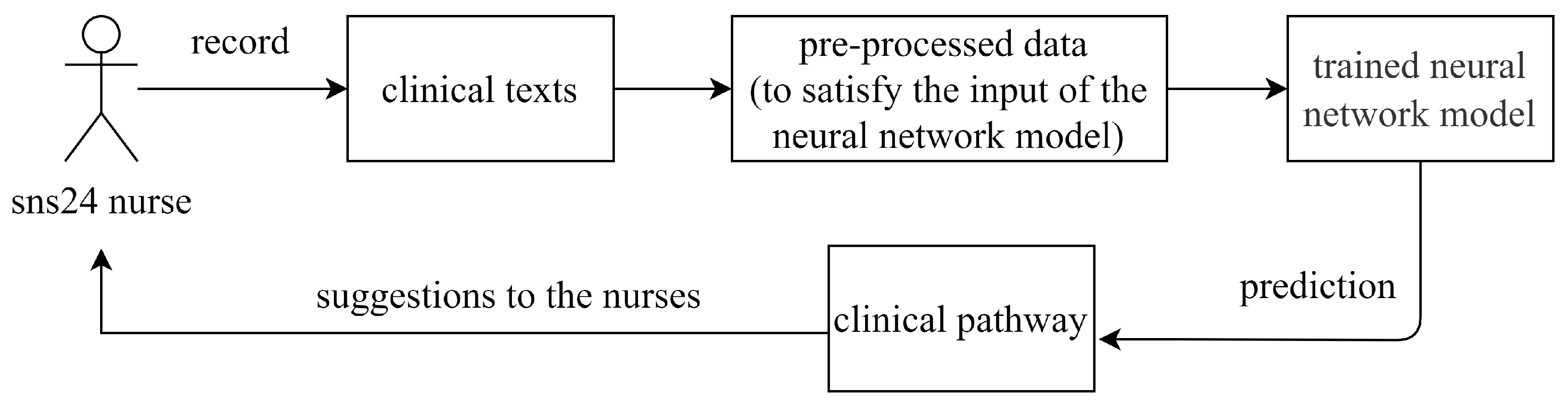
Our main task is to support the nurses with the clinical algorithm’s choice. This can be framed as a supervised multi-class classification problem using as input the dataset we obtained from SNS24 calling records. The existing clinical dataset includes clinical texts and their corresponding clinical pathways are used for training a deep neural network model. Given a new record, the attribute “clinical pathway” is the class aiming to be predicted. As Figure 1 presents, the trained neural network model is used to predict the clinical pathway given the information collected by the nursers, and the predicted clinical pathway is finally returned to the nurse as the suggestion.

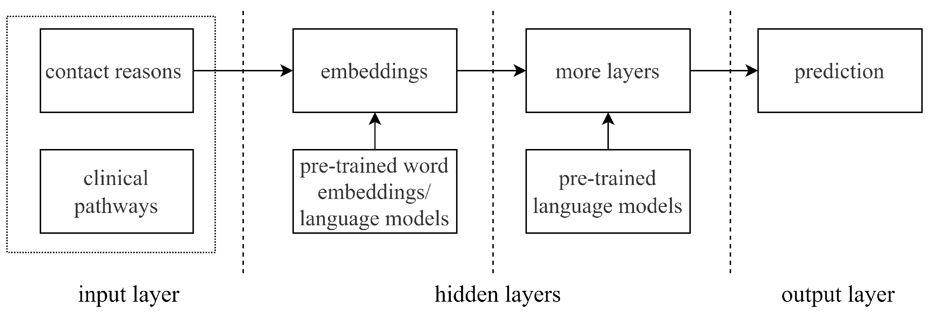
Figure 2 presents the general framework for training a neural network model in our task. The design of a neural network model is highly depending on the selected architecture, such as the number of layers, the design of hidden layers, the pre-trained language model selection, etc. We propose to train neural network models using CNN, RNN, and transformers-based architectures:

• CNN-based architecture. We use the architecture described by Yoon Kim [18], which is a classical convolutional neural network for text classification.
• RNN-based architecture. Mainly, two prevailing RNN types have been developed from the basic RNN [19]: long short-term memory (LSTM) [20] and gated recurrent unit (GRU) [21]. We use GRU type RNN in our experiments.
• Transformers-based architecture. Transformers is a sequence-to-sequence architecture that was originally proposed for neural machine translation, and it shows effective performance in natural language processing tasks [22].

As Figure 2 shows, for each architecture, “contact reason” and “clinical pathway” are used as the articles and labels. They are pre-processed and fed to the neural network as the input. When embedding the input “contact reason” texts and building other hidden layers, pre-trained language models are used depending on the neural network architecture selection.

Compared to the one-hot representation which maps words into high-dimensional and sparse data, the static distributed representation (word embeddings) maps the words into a low-dimensional continuous space and can capture the semantic meanings of words. In the scope of static distributed representations, a number of pre-trained word embeddings are available, such as Word2Vec, Glove, fastText, etc. More recently, the contextualized (dynamic) distributed representation (language models) presents the ability to encode the semantic and syntactic information [23]. For example, pre-trained language models include ELMO [24], BERT [25], XLNet [26], Flair [27,28], etc. Since both the pre-trained word embeddings and pre-trained language models are state-of-the-art techniques to transform word into distributed representations, we take both into account in our task.

4. Experiments

In this section, we start by describing the experimental setup. As the first step, we preliminarily experiment with all three neural network architectures over a small number of epochs. Based on the results obtained from the preliminary experiments, the following step is to select the best-performed architecture among all three and further fine-tuning the models with selected hyperparameters step by step. The final best fine-tuned model will be used for class prediction.

4.1. Experimental Setup

In our previous work, we used shallow machine learning approaches to predict the clinical pathways on the SNS24 dataset [17]. Different from deep learning approaches, shallow machine learning approaches or conventional machine learning approaches usually need human intervention in feature extraction. Typical shallow machine learning approaches include Linear/Logistic Regression, Decision Tree, SVM, Naive Bayes, Random Forest, etc.

To be able to compare to our previously obtained results using shallow machine learning approaches [17], we use the same train/validation/test splits of the same dataset. The dataset is stratified split into the train (64%), validation (16%), and test set (20%). The neural network models are trained over the train set and adjusted over the validation set, and the test set is used for the final evaluation of the models.

Also, we use the same field texts as used in the shallow machine learning approach. The original dataset contains 18 fields (attributes), and only the texts of the “contact reason” field and the labels of the “Clinical pathway” field are used in building a prediction model. The texts from the other fields of the dataset are not used. Example texts and labels are shown in Table A2.

We use TensorFlow 2.2, Pytorch 1.8, and Python 3.8 as the framework in building the neural network models. We mainly use two state-of-the-art NLP libraries and their pre-trained language models: Transformers https://huggingface.co/transformers/ (accessed on 2 April 2022) and FLAIR https://github.com/zalandoresearch/flair (accessed on accessed on 2 April 2022).

4.2. Preliminary Experiments

4.2.1. CNN-Based Architecture

Among a number of the convolutional neural networks (CNN) that have presented excellent performances in many natural language processing tasks, one typical CNN architecture for text classification is proposed by Kim [18]. This type of CNN architecture generally includes these layers: embedding layer (input layer), convolutional layer, pooling layer, and fully connected layer.

We build our CNN model based on this type of CNN architecture. When applying CNNs in text analysis, the input has a static size and text lengths can vary greatly [18]. So, as the input, the texts from the “contact reason” field are tokenized, and all words are integer encoded. These pre-processed train data are then fed to the CNN architecture. In the embedding layer, each word is embedded into a 200-dimension vector. A one-dimensional convolution layer is then added. Filters perform convolutions on the text matrix and generate feature maps. We depict one filter region size in our experiments. The max-pooling is performed over each feature map to select the most prominent feature (the largest number). We choose max-pooling as the pooling strategy since it presents much better performance compared to average pooling in the text classification tasks [29]. Then, the max-pooling results of word embeddings are concatenated together to form a single feature vector. To prevent the built CNN model from overfitting, we add a dropout layer after the fully connected layer [30]. The final Softmax layer receives the concatenated feature vector as input and uses it to classify the texts. The main hyperparameters settings in the built CNN model are shown in the second column of

Table 3. Hyperparameter settings in the neural network models for different architectures. The first column lists the main hyperparameters used in all three neural network architectures, and the hyperparameters that are not used or not manually set in our experiments in one architecture are marked with “-” in the table. CCEE stands for categorical cross entropy error.

Hyperparameters	CNN-Based	RNN-Based	Transformers-Based
Hidden layers	4	3	12
Hidden size	-	512	768
Filter size	3	-	-
Feature map	128	-	-
Pooling strategy	1-max pooling	-	-
Activation function	ReLU, Softmax	-	Gelu [31]
Regularization strategy	Dropout	Dropout	Dropout
Dropout rate	0.1	0.1	0.1
Batch size	128	128	128
Patience	-	5	-
Anneal factor	-	0.5	-
Optimizer	Adam	Adam	Adam
Learning rate	$1\times {10}^{-4}$	$1\times {10}^{-4}$	$1\times {10}^{-4}$
Loss function	CCEE	CCEE	CCEE
Epoch	10	10	10

.

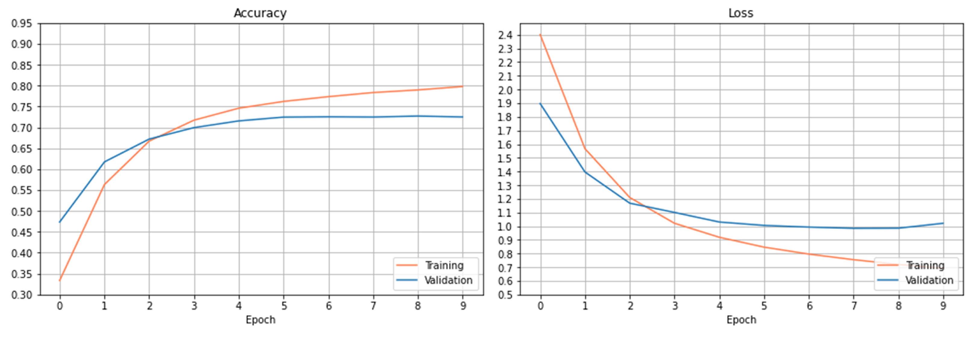
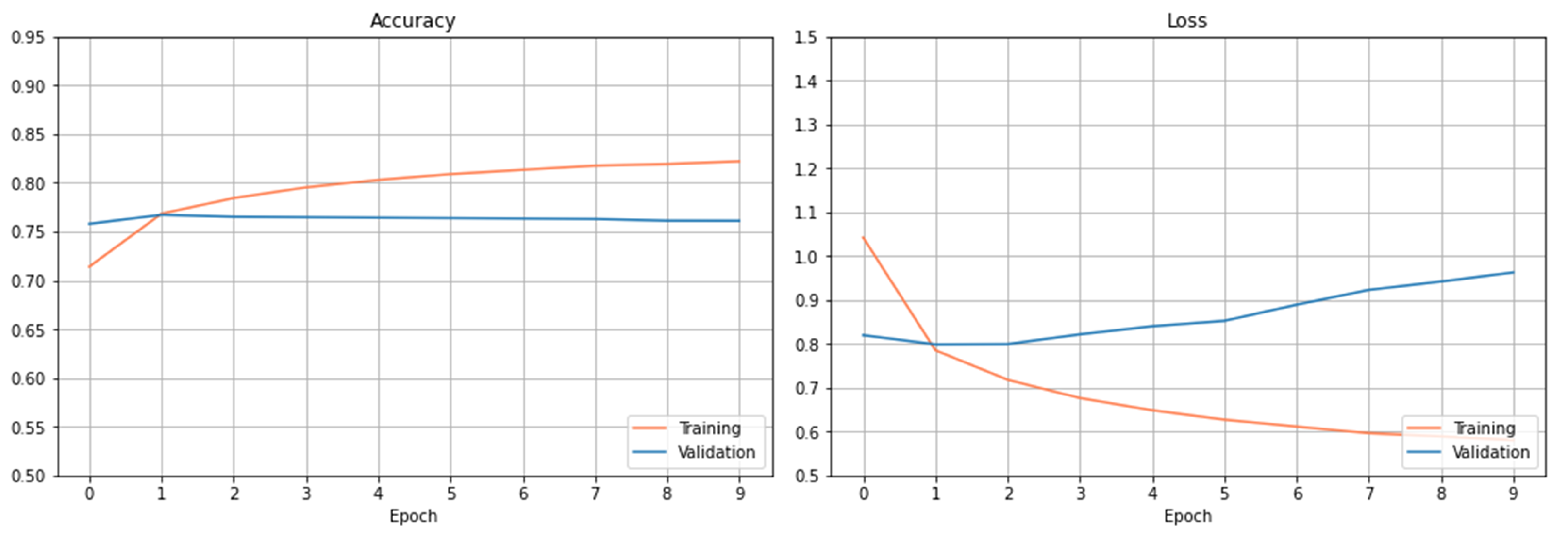
The training and validation results are presented in Figure 3. The left figure shows the accuracy’s on the train and validation datasets. As it can be observed, the accuracy increases slowly on the training dataset after 6 epochs. The accuracy on the validation dataset tends to saturate after certain epochs, and the curve doesn’t show the trend of increasing accuracy after more epochs within the setting one. Figure 3 right plots the loss curves of the train and validation datasets over the setting epochs. The loss curve on the training dataset decreases rapidly at the beginning of 3 epochs and slowly after the 3 epochs. The loss curve on the validation dataset saturates gradually after 6 epochs, and the loss has been reduced to a minimum level at epoch 8 and then begins to increase. As observed from both figures, the curves have been basically stable after 6 epochs within the setting epochs.

Using this trained CNN model, the accuracy obtained on the test dataset is 76.56%.

4.2.2. RNN-Based Architecture

When constructing the RNN-based neural network for our task, we choose to use the pre-trained Flair model as the implementation. Flair is a natural language processing (NLP) library and builds on PyTorch which is one deep learning framework. A group of pre-trained models for the NLP tasks is provided in Flair.

We choose the pre-trained Flair model that provides text classification ability as part of the implementation of our RNN-based model [28]. The pre-trained text classification model takes word embeddings, puts them into a recurrent neural network (RNN) to obtain a text representation, and puts the text representation in the end into a linear layer to get the actual class label [28]. The list of the word embeddings from one text is passed to the RNN, and the final state of the RNN is used as the representation for the whole text. The GRU-type RNN is used in our experiments. The main hyperparameters settings used are shown in Table 3.

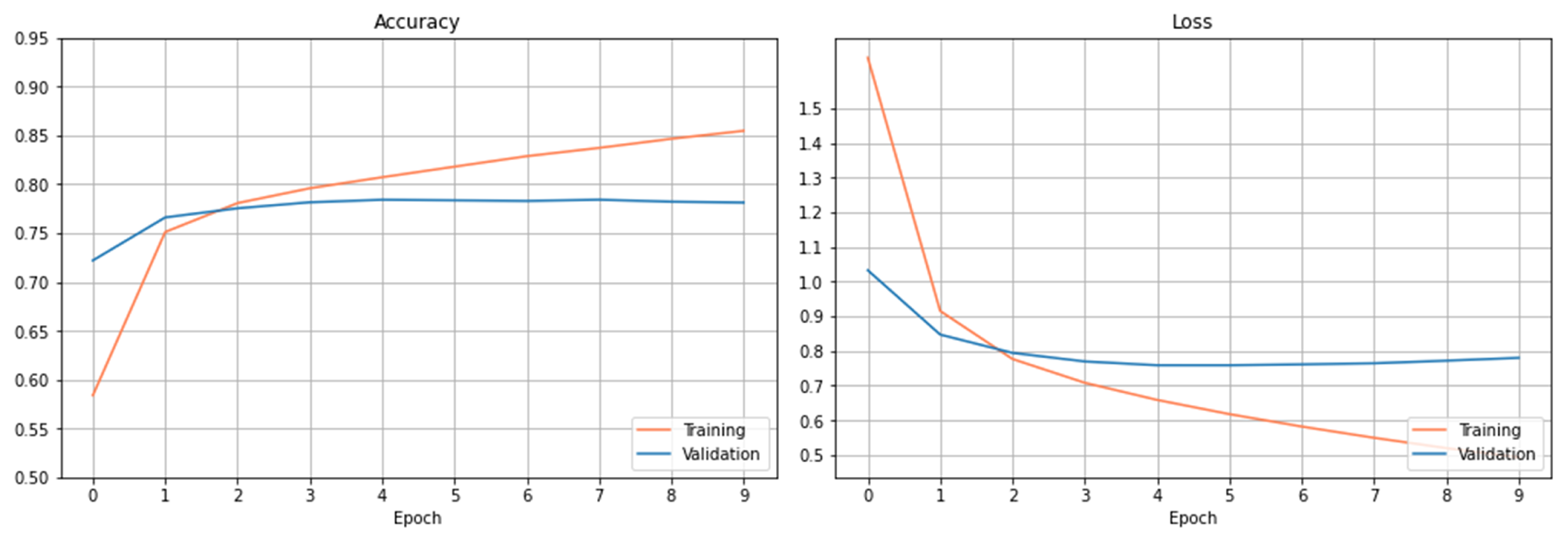
Figure 4 plots the accuracy and loss observed on the training and validation dataset using the RNN-based architecture. From the results, we can see that this model overfits too early after only a few epochs. The best score obtained on the testing dataset is 75.88%.

4.2.3. Transformers-Based Architecture

To construct the transformers-based neural network for our task, we chose to use the pre-trained BERT model as the implementation of transformers.

We choose a pre-trained BERT model that provides text classification ability [25,32]. With TensorFlow, we first instantiate this classification model with a pre-trained model’s configuration from a BERT Portuguese model; then, we fit the model to our dataset. We use BERTimbau Base, which is a pre-trained BERT model for Portuguese that achieves state-of-the-art performance on a number of NLP tasks. In particular, we use the base model of BERTimbau Base, which includes 12 layers [33]. The pre-processed data is then fed to the neural network. The main hyperparameter values used in the transformed-based architecture are summarized in the fourth column of Table 3.

Figure 5 depicts the accuracy and loss curves on the training and validation dataset. The loss on the validation dataset has been reduced to a minimum level at epoch 5. Using the transformers-based architecture, the accuracy score obtained on the testing dataset is 78.15%.

4.3. Fine-Tuning of the Transformers-Based Models

In our preliminary experiments, we use the default or empirical hyperparameter settings when building a prediction model. To adapt the neural network models to our task, we fine-tune the hyperparameter to our target dataset.

Since the transformers-based model presents better performance than the CNN and RNN models in the preliminary experiments, we further fine-tune the hyperparameters of the transformers-based model, aiming to achieve better results.

4.3.1. Fine-Tuning Strategy

Our fine-tuning aim is: (1) an ideal optimizer with an appropriate learning rate; (2) an ideal batch size for training on the target dataset. So, we mainly consider three hyperparameters, learning rate, optimizer, and batch size.

Since it is costly to train transformers-based models, the fine-tuning process is designed as the following:

• Fine-tuning of learning rate (abbr. lr). During the first phase, we experiment with small epochs (e.g., 10) and range with different learning rates on the different optimizers.
• Fine-tuning on epochs. Based on the results observed from the first phase, we analyze the accuracy and loss curves to choose the best learning rate for each optimizer. We then use that group of hyperparameters and set the epoch to a large number for further training.
• Fine-tuning on batch size. Based on the results obtained after fine-tuning on learning rates and epochs, the final fine-tuning is done by adjusting the batch size with a set of varying values.

In such a way, we can better save the resources in training the models and shorten the time in fine-tuning. This method practically eliminates the need to repeatedly tune on large epochs every time and theoretically achieves near-optimal classification accuracy. We will describe each phase strategy in more detail in the following subsections.

4.3.2. Optimization Algorithm Choosing

The optimization algorithm (a.k.a. optimizer) is one main approach used to minimize the error when training neural network models. A number of optimizers have been researched and generally used ones include Stochastic Gradient Descent (SGD), Momentum Based Gradient Descent, Mini-Batch Gradient Descent, Nesterov Accelerated Gradient (NAG), Adaptive Gradient Algorithm (AdaGrad), Adaptive Moment Estimation (Adam), etc. [34,35,36,37]. When choosing an optimizer for fine-tuning the neural network models, the speed of convergence and the generalization performance on the new data are usually considered.

In our work, we mainly take into account two widely used optimizers in our experiments, Adaptive Moment Estimation (Adam) [34] and Stochastic Gradient Descent (SGD) [37] since these two optimizers present better performances than the others in many NLP tasks. When training neural network models, Adam is one of the most practical optimizer. Adam is an algorithm for gradient-based optimization and combines the advantages of two SGD extensions: RMSProp and Adagrad [34]. Adam can compute adaptive learning rates for different parameters individually. As a variant of Gradient Descent (GD), SGD is a computationally efficient optimization method on large-scale datasets. When doing experiments on a large-scale dataset, computations over the whole dataset are usually redundant and ineffective. SGD can do computations on a small or a randomly selected subset instead of the whole dataset [37].

4.3.3. Fine-Tuning of Learning Rate

During this phase, we explore the effect of different learning rate settings. In particular, we focus on the variants of the learning rate with each optimizer.

The setting of the learning rate plays a decisive role in the convergence of a neural network model. A too-small learning rate will make a training algorithm converge slowly, while a too-large learning rate will make the training algorithm diverge [38]. A traditional default value for the learning rate is 0.1, and we use this as a starting point on our task problem [38,39]. For each optimizer (Adam and SGD), we try learning rates within the set of {0.1, 0.01, $1\times {10}^{-3}$, $1\times {10}^{-4}$, $1\times {10}^{-5}$, $1\times {10}^{-6}$, $1\times {10}^{-7}$}. We maintain the same training procedure as the preliminary models described in Section 4.2.3 except for changing the learning rate. We use the same number of epochs (epochs = 10) as a start. The rest of the hyperparameters remain the same (see Section 4.2.3).

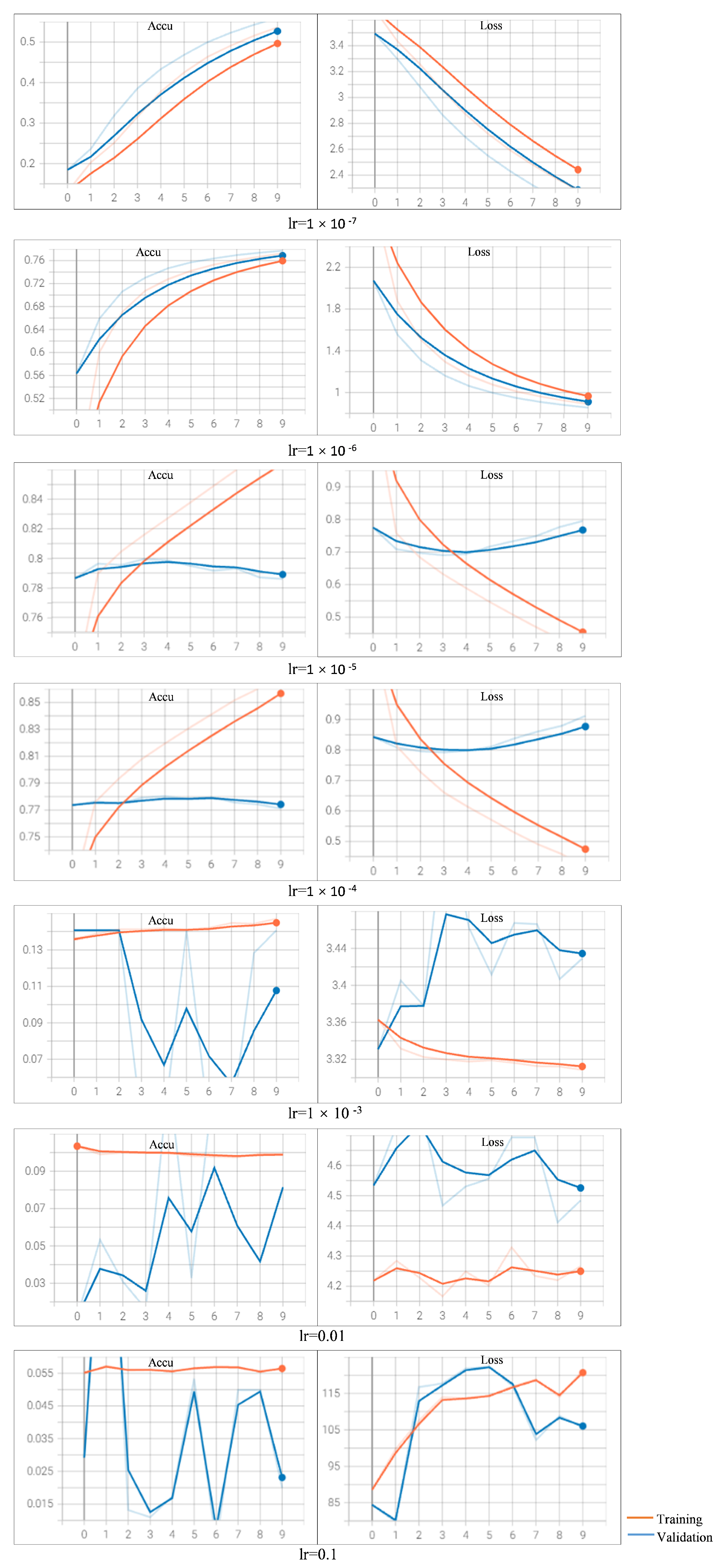
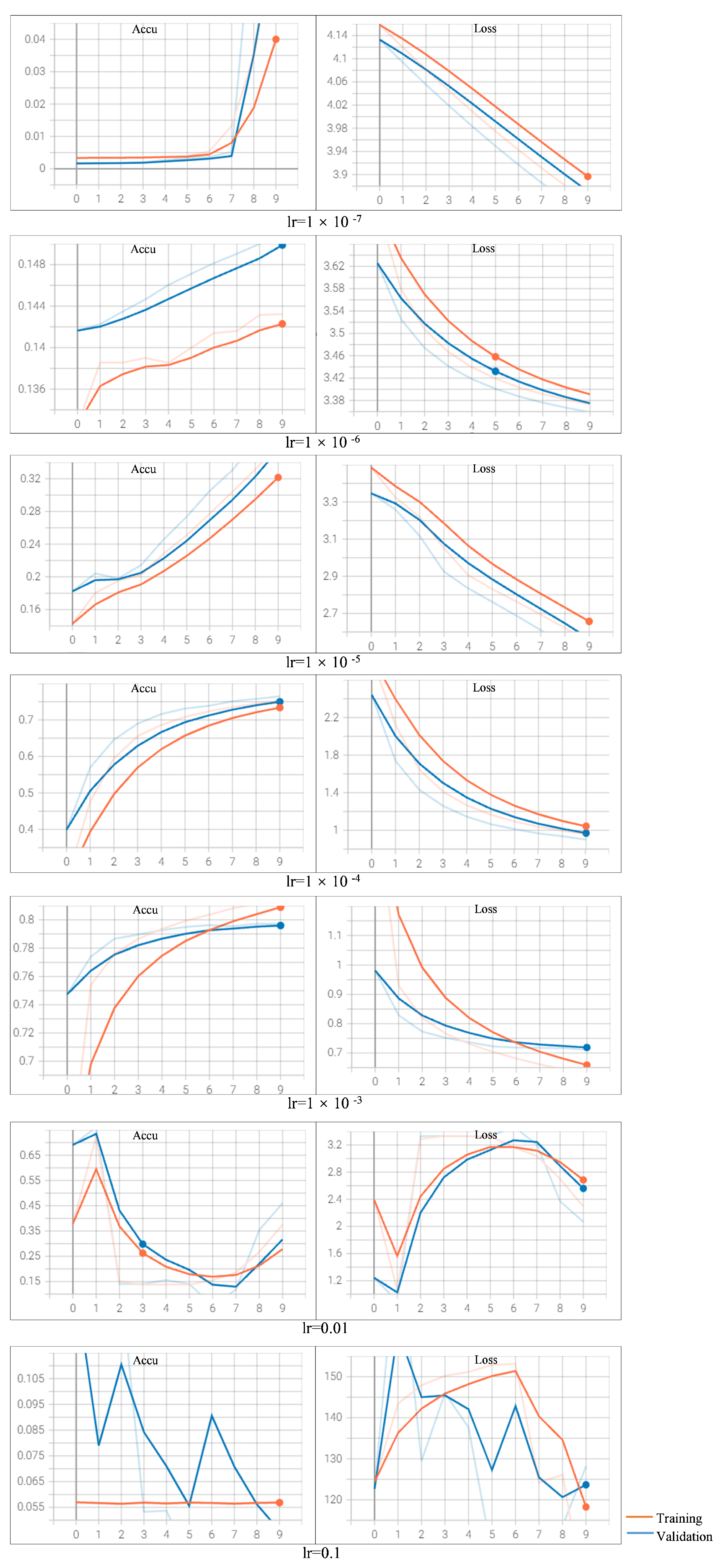
When varying the learning rate settings with optimizer Adam (Figure A1) and SGD (Figure A2), the training and validation curves of the train and validation dataset are depicted. The results on accuracy as well as loss values are reported.

Observing the curves learned by using Adam with different learning rates, we find that when setting the learning rate as $1\times {10}^{-3}$ or bigger, the training models fails to converge (refer Appendix B Figure A1). Especially when the learning rate is set with an aggressive value of 0.1, we observe that the loss increases rather than decreases. When the value is set as $1\times {10}^{-4}$ or $1\times {10}^{-5}$, the two models archive similar performance, and the models converge too early on the validation dataset. We also observe that the loss on the validation dataset increases with more epochs. When setting a rather small value of $1\times {10}^{-7}$, we observe that the loss decreases too slow compared to the other learning rates (the loss is around 2.3 after 10 epochs). When setting the learning rate as $1\times {10}^{-6}$, we observe that the results clearly show a downward trend in loss and upward in accuracy over the epochs. This sign shows the model is learning the problem and has learned the predictive skill.

So, when choosing Adam as the optimizer, the appropriate setting of learning rate is $1\times {10}^{-6}$. The loss curves of the training and validation datasets are decreasing, and they are still showing downward trends by the pre-defined epochs. This observation suggests that the prediction performance could be potentially improved with more epochs (training with more epochs than 10). The best accuracy on the test dataset achieves a score of 79.67%, obtained with the learning rate of $1\times {10}^{-5}$ and Adam optimizer.

When varying the learning rate setting with optimizer SGD, we can analyze the results similarly as with the Adam optimizer (refer Appendix B Figure A2). We observe that the model fails to converge when the learning rate is set as 0.1 or 0.01; the model converges too early with a learning rate of $1\times {10}^{-3}$; the loss decreases very slow when the learning rate is $1\times {10}^{-5}$ or smaller. The best accuracy on the test dataset achieves a score of 79.72%, obtained with the learning rate of $1\times {10}^{-3}$ and SGD optimizer. But the curve shows no obvious downward trend on $1\times {10}^{-3}$ after 10 epochs. So, with SGD as the optimizer, the appropriate learning rate setting is $1\times {10}^{-4}$.

4.3.4. Fine-Tuning on Epochs

Based on the results observed on fine-tuning of the learning rates, we focus on adjusting the number of training epochs during this phase.

We observe that the results clearly show a downward trend in loss and upward in accuracy with the learning rate of $1\times {10}^{-6}$ on Adam optimizer (see Figure A1). This trend suggests that continuing to increase the value of epochs can potentially further improve the performance of the model [40]. Although the best testing accuracy is obtained with a learning rate of $1\times {10}^{-5}$, its learning curve doesn’t show an obvious downward trend (see Figure A1). 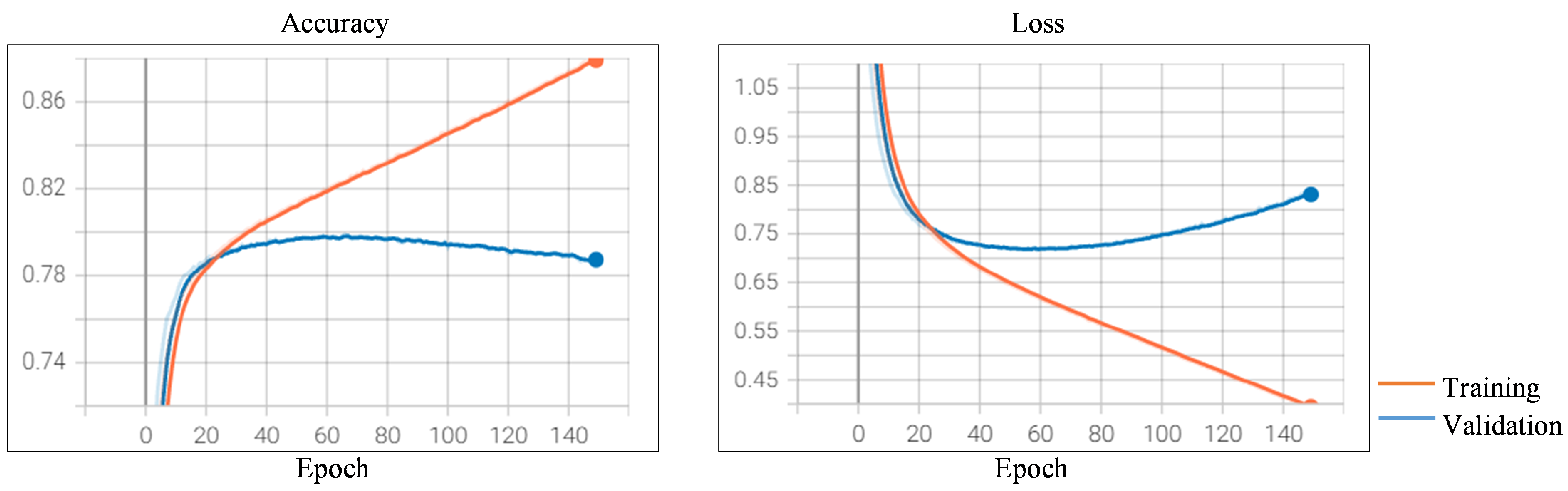So, we choose the learning rate of $1\times {10}^{-6}$ for further fine-tuning. We experiment by increasing the number of epochs from 10 to 150 and keeping the other hyperparameters the same. 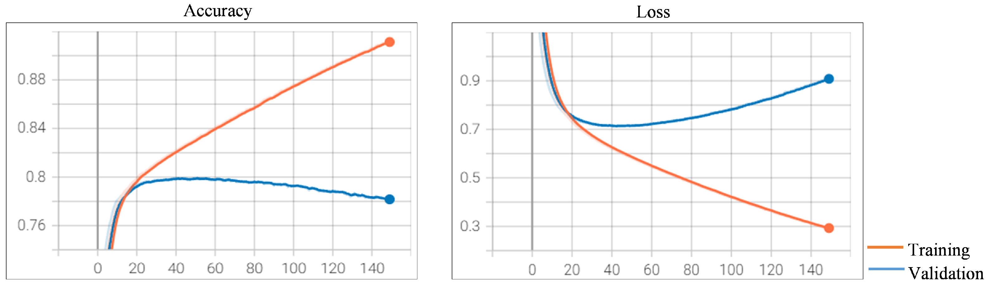The training and validation curve is presented in Figure 6. The increasing trend of the loss on the validation dataset is a sign of overfitting. As presented in Figure 6, the loss curve shows the beginnings of this type of pattern after 41 epochs. This is where the model overfits the training dataset at the cost of worse performance on the validation dataset. These observations suggest that the best prediction model can be obtained after 41 epochs. The accuracy on the test dataset achieves a score of 79.96%.

Now we turn to the model trained with the SGD optimizer. As the loss decreases most quickly on SGD is when setting the learning rate to $1\times {10}^{-4}$ (see Figure A2). Similar to the experiment carried out on Adam, we use SGD as the optimizer and set the learning rate to $1\times {10}^{-4}$. The results after 150 epochs are presented in Figure 7. we also observe that the runs show the beginnings of overfitting on the validation dataset after 67 epochs, and the best prediction model can be potentially obtained after 67 epochs. The accuracy on the test dataset achieves a score of 79.76%.

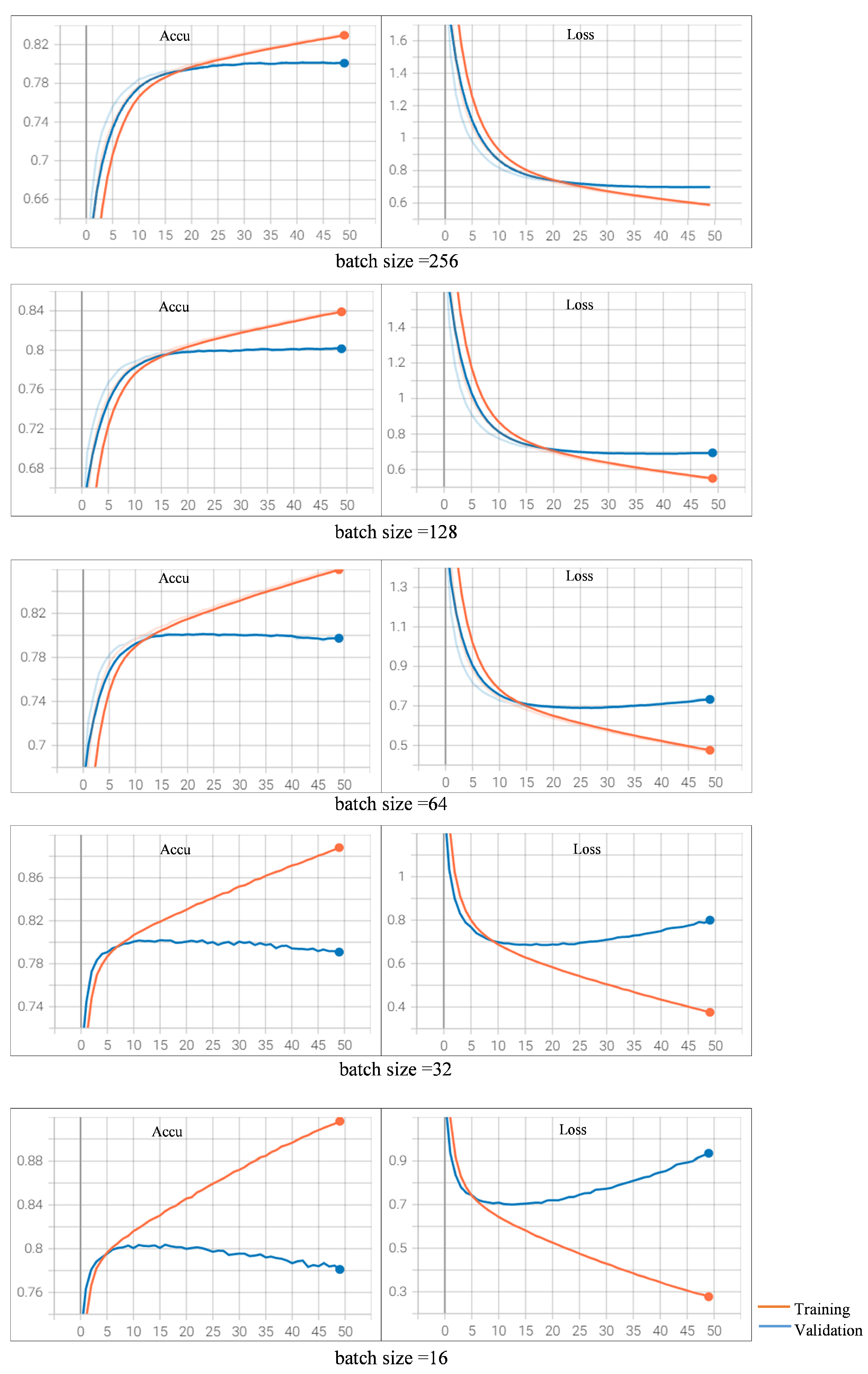
4.3.5. Fine-Tuning on Batch Size

As found by Smith and Le [41], small batch size can improve the performance, we further fine-tune our models by choosing different batch sizes within the set of {256, 128, 64, 32, 16}. Since the model trained with Adam optimizer and the learning rate of $1\times {10}^{-6}$ is able to achieve better results than the other models after 150 epochs, the final tuning is carried out on this model.

As observed in Figure 6, the validation accuracy does not change too much and begins to drop after 41 epochs, which means the model begins to converge. So, we choose the epoch of 50 on our final tuning within the batch size set (refer Appendix B Figure A3). The model trained with a batch size of 16 is able to surpass all the other models. The accuracy on the test dataset achieves a score of 80.57%.

In summary, all the models trained during the fine-tuning process are evaluated in testing accuracy and the results are presented in

Table 4. Model results obtained during the fine-tuning process. All the models use the transformers-based architecture. The hyperparameters that are not listed in this table use the same settings presented in Table 3.

Optimizer	Learning Rate	Epochs	Batch Size	Testing Accuracy
Adam	0.1	10	128	6.57%
Adam	0.01	10	128	9.05%
Adam	$1\times {10}^{-3}$	10	128	14.02%
Adam	$1\times {10}^{-4}$	10	128	78.01%
Adam	$1\times {10}^{-5}$	10	128	79.67%
Adam	$1\times {10}^{-6}$	10	128	76.57%
Adam	$1\times {10}^{-7}$	10	128	52.32%
SGD	0.1	10	128	12.12%
SGD	0.01	10	128	73.76%
SGD	$1\times {10}^{-3}$	10	128	79.72%
SGD	$1\times {10}^{-4}$	10	128	75.01%
SGD	$1\times {10}^{-5}$	10	128	38.89%
SGD	$1\times {10}^{-6}$	10	128	15.01%
SGD	$1\times {10}^{-7}$	10	128	6.26%
Adam	$1\times {10}^{-6}$	150	128	79.96%
SGD	$1\times {10}^{-4}$	150	128	79.76%
Adam	$1\times {10}^{-6}$	50	16	80.57%
Adam	$1\times {10}^{-6}$	50	32	80.19%
Adam	$1\times {10}^{-6}$	50	64	80.20%
Adam	$1\times {10}^{-6}$	50	128	80.25%
Adam	$1\times {10}^{-6}$	50	256	80.08%

.

5. Results and Discussion

We consider three deep neural network architectures in our experiments. We use these neural networks combined with different representations for words and texts. These built models and their respective testing accuracies results are presented in

Table 5. Results comparison among the three deep learning architectures.

Deep Learning Architecture	Fine-Tuned Hyperparameters	Testing Accuracy
CNN-based architecture	-	76.56%
RNN-based architecture	-	75.88%
Transformers-based architecture	-	78.15%
	learning rate	79.67% (Adam, lr = $1\times {10}^{-5}$)
	learning rate	79.72% (SGD, lr = $1\times {10}^{-3}$)
	epochs	79.96% (Adam, epochs = 150)
	epochs	79.76% (SGD, epochs = 150)
	batch size	80.57%

.

Among them, the transformers-based model using BERT-base language model achieves a result of 78.15%. The CNN-based approach achieved an accuracy of 76.56%, and the RNN-based approach achieved an accuracy of 75.88%. The transformers-based approach is shown to be better than the one using the CNN-based or RNN-based approach. We then fine-tune the transformers-based models. A better model with a higher accuracy score is obtained after we fine-tune the hyperparameters on learning rate, optimizer, number of epochs, and batch size step by step. The best fine-tuning model achieves an accuracy of 80.57% on the testing set.

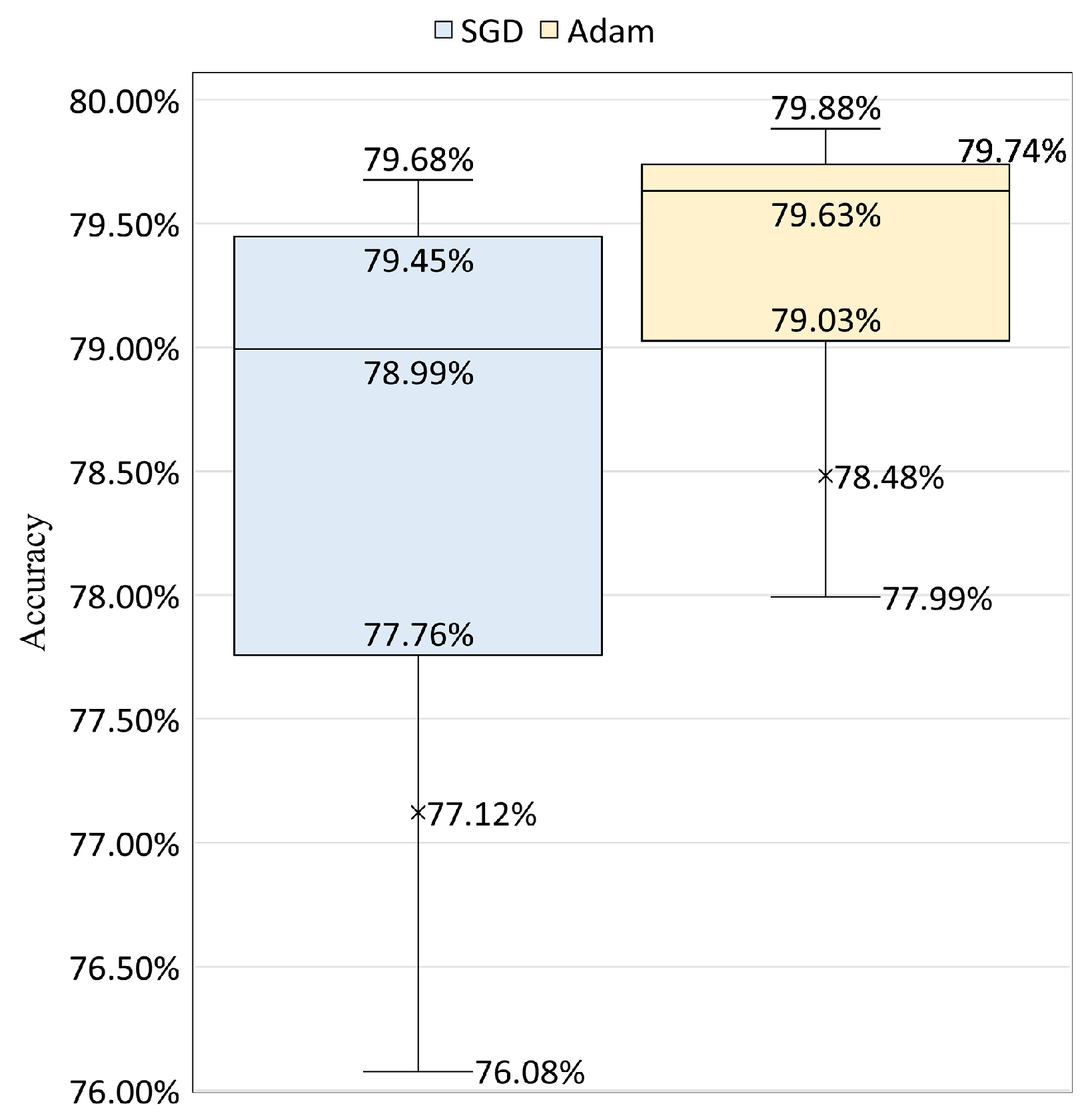
We also compare the performance between the Adam and SGD optimizers using their validation accuracy distributions over the 150 epochs. In Figure 8, we present the results with a box plot using the data that both optimizers achieve with their best learning rate, where Adam has a learning rate of $1\times {10}^{-6}$ and SGD has a rate of $1\times {10}^{-4}$ The outliers that are smaller than the minimum for both optimizers are removed in the figure for a clear presentation. This does not affect the comparison between the distributions. We choose a learning rate of $1\times {10}^{-6}$ for Adam and $1\times {10}^{-4}$ for SGD because their learning curves show clear downward trends in losses and upward trends in accuracies. Also, they are able to achieve comparative performances compared to other learning rates (see Figure A1 and Figure A2).

We observe that the model with Adam optimizer achieves better top accuracy on the validation dataset than the model with SGD. Besides, when comparing Figure 6 and Figure 7, Adam has been found to attain the top accuracy performance with a smaller number of epochs necessary (epoch = 41), while SGD requires more to converge (epoch = 47).

These findings suggest that: (i) The value of the learning rate and the optimizer choice can have a strong influence on each other, in other words, the performance of the built models highly depends on the combination of the learning rate and the optimizer; (ii) With the appropriate learning rate setting, Adam outperforms SGD not only in final generalization performance but also able to converge with a smaller number of epochs.

In our previous work [17], we have explored using shallow machine learning techniques to build prediction models on the SNS24 clinical triage classification task. Four shallow machine learning algorithms were used in the previous work: linear SVM, RBF kernel SVM, Random Forest, and Multinomial Naïve Bayes [17]. For the features, we used word n-grams with word counts and TF-IDF; we also used word embeddings built with BERT [25] and Flair [27] models. The experiments carried out in this work use the same dataset and train/val/test splits. The performances between the shallow machine learning techniques and neural networks are presented in

Table 6. Comparison between the neural network and shallow machine learning techniques on the SNS24 clinical triage classification task.

Machine Learning Techniques	Architecture/Algorithm	Testing Accuracy
Neural network	CNN-based architecture	76.56%
	RNN-based architecture	75.88%
	Transformers-based architecture	80.57%
Shallow machine learning	Linear SVM	77.96%
	RBF SVM	76.97%
	Random Forest	74.93%
	Multinomial NB	66.26%

.

We can see that the transformers-based architecture achieves the highest score of all the experimented techniques, and was able to surpass the other two neural network architectures and the linear SVM algorithm, presenting the best among the four shallow machine learning techniques.

6. Analysis among Similar Clinical Symptoms

In this section, we performed an analysis of the trained neural network models when dealing with classes that have similar clinical symptoms. According to the SNS24 call center, there is some degree of overlap between clinical pathways. Although this overlap is expected, it may make cause the clinical decision making process to be more complex. Figure 9 and Figure 10 presents two example groups that includes clinical pathways with similar symptoms.

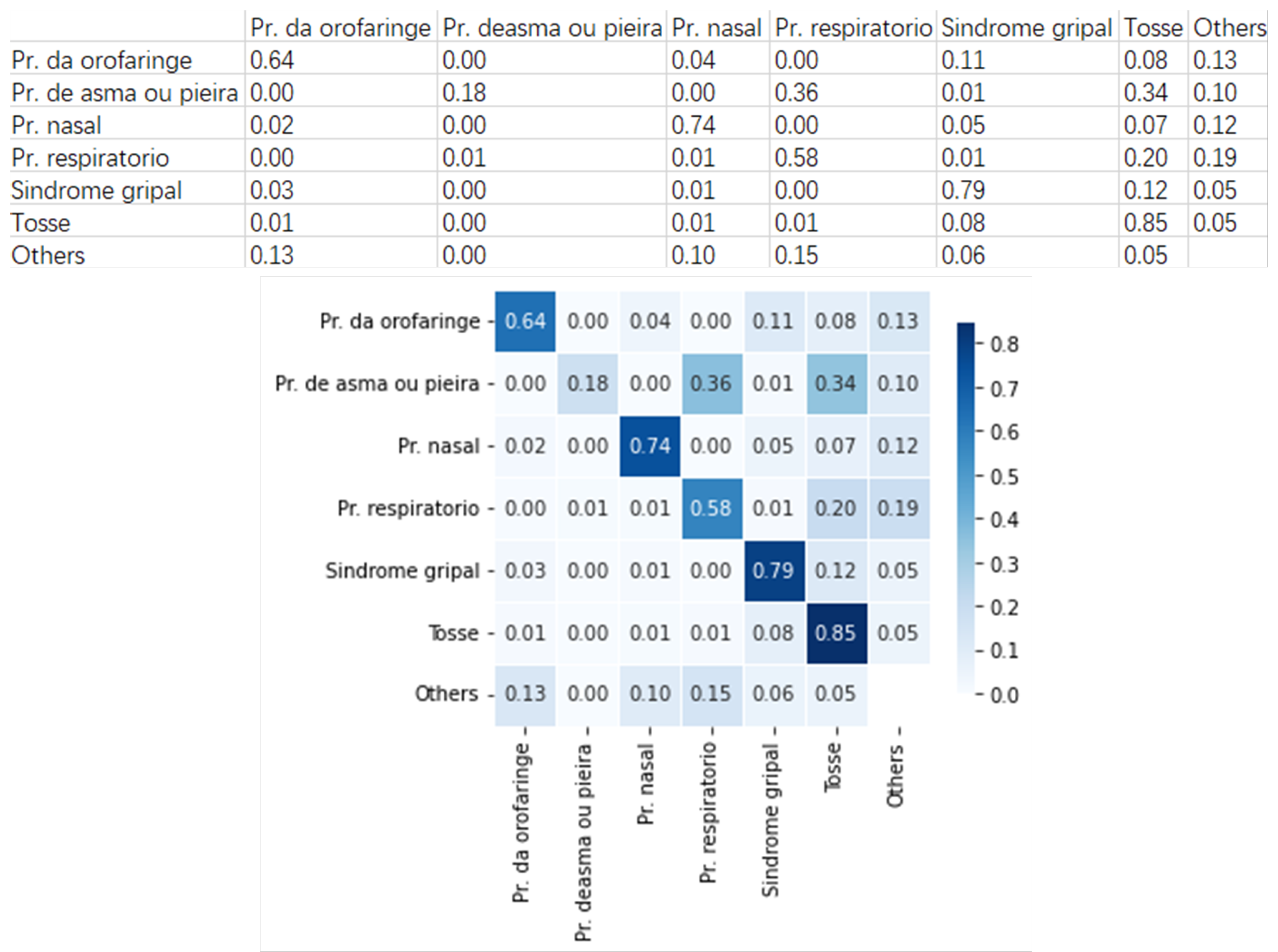
Figure 9 presents an example group that includes six clinical pathways with similar symptoms. They are Pr. da orofaringe (Oropharynx problem), Pr. deasma ou pieira (Asthma or wheezing problem), Pr. nasal (Nasal problem), Pr. respiratorio (Respiratory problem), Sindrome gripal (Flu syndrome), and Tosse (Cough).

Using the pre-trained neural network model, we built the heatmap for these clinical pathways. Taking Oropharynx problem for example, 64% of the cases are rightly classified, 4% are wrongly classified as Nasal problem, 11% as Flu syndrome, 8% as Cough, and 13% as the other clinical pathways. On the other way around, 3% Flu syndrome cases are wrongly classified as Oropharynx problem, and 12 % as Cough.

These observations suggest that Flu syndrome cases are more likely to be classified as Cough than Oropharynx problem. But on the other way, the Oropharynx problem case is more likely to be classified as Flu syndrome than Cough. Furthermore, we find that 1% of the Cough cases are wrongly classified as Oropharynx problem and 8% as Flu syndrome, which means that Cough cases are more likely to be classified as Flu syndrome.

Joining these above observations, we can deduce that it is harder to distinguish between Cough and Flu syndrome cases, and in practical application, the nurses should pay more attention to identifying these two types of clinical pathways.

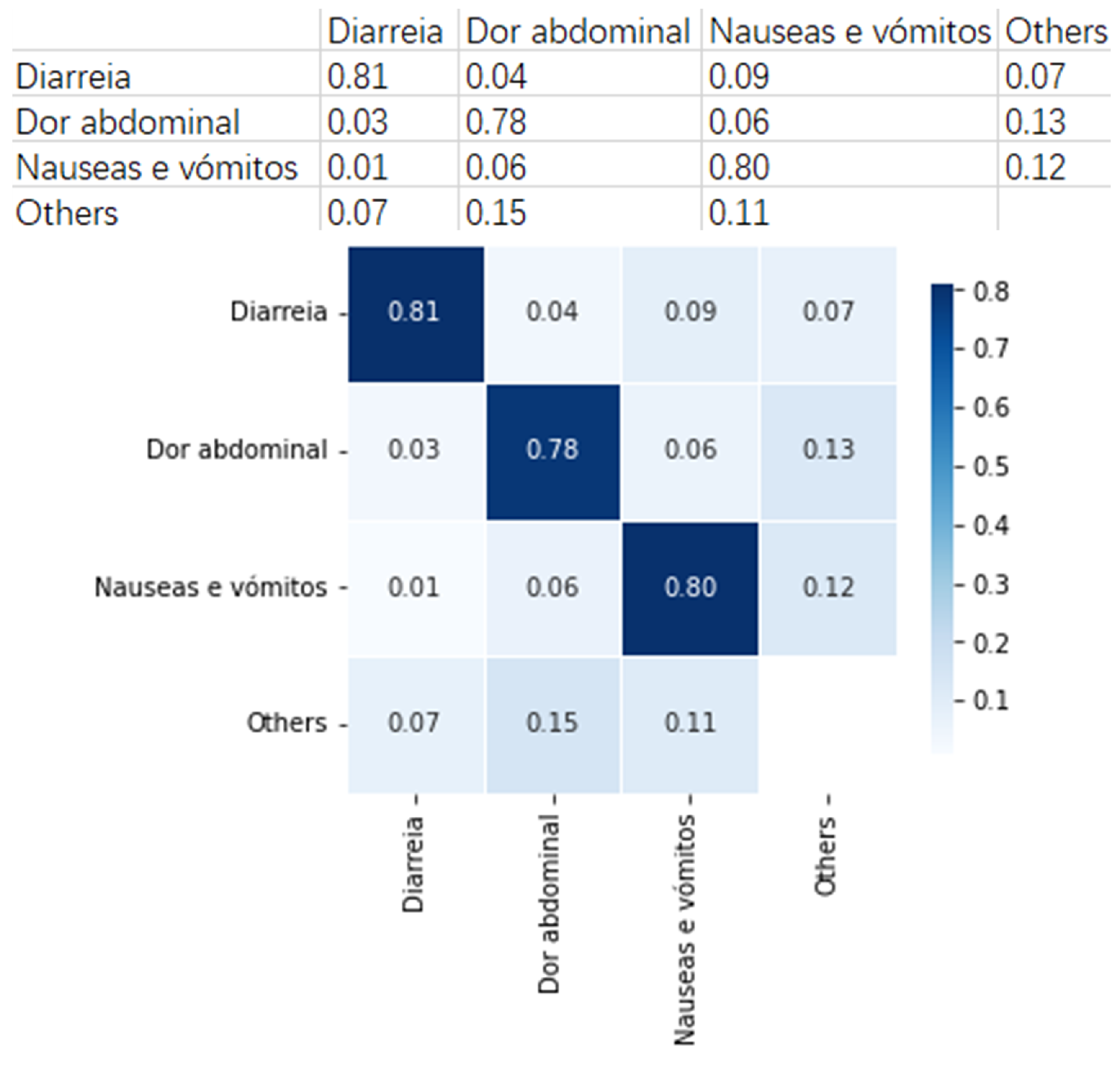
Figure 10 presents an example group that includes three clinical pathways with similar symptoms. They are Diarreia (Diarrhea), Dor abdominal (Abdominal pain), and Náuseas e vômitos (Nausea and vomiting).

As can be observed, an average of 80% cases in this group can be rightly classified with the built neural network model. This means that the built model can provide useful suggestions to the SNS24 nurses when distinguish the clinical pathways that fall into this group.

We also find that for Abdominal pain, 6% are wrongly classified as Nausea and vomiting, and 3% as Diarrhea. This means that Abdominal pain is more likely to be classified as Nausea and vomiting. Similarly, when observing Nausea and vomiting, 6% are classified as Abdominal pain and 1% as Diarrhea. These findings suggest that Abdominal pain and Nausea and vomiting cases are harder to be distinguished in this group. These results provide valuable analysis for the SNS24 Health Calls center, for example, helping to do deep analysis between similar symptoms.

7. Analysis of Individual Predictions

In this section, we aim to compare the labels ascribed by the neural network model and the support vector machines predictions (model from previous work) with the original labels.

Over time, the number of different nurses working in the health line is very high, and some nurses can be biased in the selection according to their experience or other factors. For example, in the 3-month period of the collected data, 588 nurses attended calls and chose the most adequate clinical pathway according to their insight.

This analysis was done for the ten clinical pathways with most records in the dataset, selecting ten examples from each class where the “contact reason” text had no common words with the clinical pathway. This resulted in a set of 100 examples.

From the comparison between the triage given by the phone line and the two ML “experts”, we observe that both ML models agree on 78 and all three agree on 49 examples out of the 100 examples; the SVM model agrees with the original triage in 53 examples, while the NN model agrees with the original triage in 55 examples.

Table 7. Agreements between SNS24 triage, neural network, and SVM experts for 20 examples. The Id column indicates the texts that the experts agreed with, and the referring text can be found with the Id in Table A2. The Count column calculates the total number of agreements among the experts.

Agreement	Id	Count
all experts	1, 6, 9, 11, 13, 15	6
triage, NN	7	1
triage, SVM	12	1
SVM, NN	2, 3, 5, 8, 10, 14, 16, 19	8
none	4, 17, 18, 20	4

resumes the agreements between experts for a sub-sample containing 20 examples (Table A2 presents the “contact reason” of each example along with the clinical pathway selected by the nurse;

Table A3. Examples and corresponding clinical pathways and labels predicted by SVM (Support vector machines) and NN (Neural Network).

Id	Clinical Pathway	SVM Prediction	NN Prediction
1	Cough	Cough	Cough
2	Cough	Nasal problem	Nasal problem
3	Nausea and vomiting problems	Nonspecific problems	Nonspecific problems
4	Nausea and vomiting problems	Allergy problem	Nonspecific problems
5	Abdominal pain	Abdominal pain	Body temperature change problem
6	Abdominal pain	Abdominal pain	Abdominal pain
7	Oropharynx problem	Oropharynx problem	Oropharynx problem
8	Oropharynx problem	Face problem	Oropharynx problem
9	Rash	Rash	Rash
10	Rash	Woman health problem	Woman health problem
11	Flu syndrome	Flu syndrome	Flu syndrome
12	Flu syndrome	Flu syndrome	Oropharynx problem
13	Urinary Problem	Urinary Problem	Urinary Problem
14	Urinary Problem	Woman health problem	Woman health problem
15	Diarrhea	Diarrhea	Diarrhea
16	Diarrhea	Nausea and vomiting problems	Nausea and vomiting problems
17	Chest pain	Nonspecific problems	Breathing problem
18	Chest pain	Pregnancy problem, puerperium	Lower limb problems, Hip
19	Migrain	Chest pain	Chest pain
20	Migrain	Cough	Flu syndrome

presents the corresponding labels given by the ML models).

It is interesting to look at the text where both ML models agree but disagree with the triage. In example 2 both classify it as Nasal problem whereas the triage classify it as Cough. The text mentions “rhinorrhea” and no cough related symptoms. Also example 3, “Lack of appetite 6 h ago”, is classified as Nonspecific problems while triage selected Nausea and vomiting problems. In fact, there is no word in the text that gives a hint about nausea.

On the other hand, there are examples where the ML experts select pathways that have close connection to words appearing in the “contact reason”: example 5 is classified by both models as Pregnancy problem, puerperium while the Abdominal pain pathway was chosen on triage and the “contact reason” text includes the word “pregnancy”; examples 8 and 14, that include the words “vaginal” and “blood loss”, respectively, are classified by both models as Woman health problem while the pathways chosen on triage were Oropharynx problem and Urinary problem, respectively.

Nonetheless, sometimes they seem to be too biased: for example, the contact reason with text “itching starting 3 days ago, in the armpits and genital region” (example 10) is classified as Woman health problem, but there’s no body part mentioned specific to women.

Sometimes we see some ambiguity, as in example 16, which both models classify as Nausea and vomiting problems, while the triage selected Diarrhea and the text includes both the words “vomiting” and “diarrhea”.

On example 7, with text “Canker sores 1 day ago, fever 2 days ago”, the NN agrees with the triage on the pathway Oropharynx problem while NN chooses Face problem for example 12, with text “sore throat since Friday and fever 38.7”, SVM is the model that agrees with the triage on Flu syndrome while NN chooses Oropharynx problem.

Two examples where the three experts disagree have triage as Chest pain. In example 17 with text “Easy fatigue 1h ago, with irradiation”, SVM classified as Nonspecific problems while NN as Breathing problem; in example 18 with text “Flank pain since 15 days pregnant”, SVM classified as Pregnancy problem, puerperium and NN as Lower limb problems, Hip.

8. Conclusions and Future Work

SNS24 is a telephone and digital public service which provides clinical services. SNS24 plays a significant role in identifying users’ clinical situations according to their symptoms. There are a group of possible clinical algorithms defined at present, and choosing the appropriate clinical algorithm is important in each telephone triage.

We carried out experiments on a dataset containing 269,654 call records belonging to 51 classes. Each record is labeled with a clinical pathway chosen by the nurse that answered the call. Three neural network architectures were trained to produce classification models. CNN, RNN, and transformers-based approaches achieve accuracies of 76.67%, 78.03%, and 78.15%, respectively. The best performance obtained, with an accuracy of 80.57%, was reached using a fine-tuned transformers-based model. The fine-tuning strategy used showed up to be efficient to improve the model performance. Also, the experiments revealed that, when setting the appropriate learning rate, the Adam optimizer achieved better performance compared to SGD. These results suggest that using deep learning is an effective and promising approach to aid the clinical triage of phone call services.

We carried out further analysis using the fine-tuned neural network models. We used the trained model to analyze similar clinical symptoms. These results provide valuable analysis for the SNS24 Health Calls center to do deep analysis among similar symptoms. We also compared the predictions from the neural network model, the support vector machines model from our previous work, and the original labels provided by SNS24.

As future work, and since the neural network models performed well on the SNS24 clinical trial classification task, we intend to fine-tune these models with other hyperparameters besides the ones explored in this work. As a continuation of the work, we plan to build models using a much larger SNS24 dataset that includes three full years of data. To support the choices made by ML models and better understand why one clinical pathway is chosen over others, we intend to apply explainable artificial intelligence (XAI) techniques.

Pursuing the line of work from Section 7 we intend to use a new subset of examples and extend the presented comparisons to the new models being created with the three-years dataset, as well as adding the insight from a few experienced nurses from the health-line.