Education 4.0: Teaching the Basics of KNN, LDA and Simple Perceptron Algorithms for Binary Classification Problems

Abstract

One of the main focuses of Education 4.0 is to provide students with knowledge on disruptive technologies, such as Machine Learning (ML), as well as the skills to implement this knowledge to solve real-life problems. Therefore, both students and professors require teaching and learning tools that facilitate the introduction to such topics. Consequently, this study looks forward to contributing to the development of those tools by introducing the basic theory behind three machine learning classifying algorithms: K-Nearest-Neighbor (KNN), Linear Discriminant Analysis (LDA), and Simple Perceptron; as well as discussing the diverse advantages and disadvantages of each method. Moreover, it is proposed to analyze how these methods work on different conditions through their implementation over a test bench. Thus, in addition to the description of each algorithm, we discuss their application to solving three different binary classification problems using three different datasets, as well as comparing their performances in these specific case studies. The findings of this study can be used by teachers to provide students the basic knowledge of KNN, LDA, and perceptron algorithms, and, at the same time, it can be used as a guide to learn how to apply them to solve real-life problems that are not limited to the presented datasets.

1. Introduction

Currently, society is going through the fourth industrial revolution, also known as Industry 4.0. This new revolution is being driven, principally, by advancements in areas such as artificial intelligence (AI), robotics, cloud computing, the internet of things (IoT), cyber-physical systems, big data, etc. [1,2]. Thus, industries have used these technologies to provide solutions to the growing needs of humankind; however, in order for them to continue adapting their ecosystems to the digital world, they need qualified professionals with knowledge and skills in those areas.

Consequently, in order to generate skillful personnel, Education 4.0 is being proposed as a new framework so that schools are able to train professionals who are capable of creating knowledge through scientific research and experience, as well as sharing this knowledge with society and using it to face technological, social, political, and economic challenges [3]. Hence, it has been of great importance for universities to develop new curricula at the undergraduate level that guide future professionals towards the requirements of Industry 4.0 [4].

Some authors have explored and proposed guidelines for the creation of newly updated curricula that are in line with the upcoming revolution. According to [3], it is important for Education 4.0 paradigm to be based on competency development so that students do not only memorize and repeat data but also learn how to use it through learning experiences. In other words, students must learn by doing, using, and interacting with material that encourages them to apply the acquired theoretical knowledge [5].

In this paradigm, we can consider the term “competency” as the set of skills, values, and knowledge that allows the student to successfully perform a given task or activity [6]. In order to develop the Education 4.0 curricula for engineers, ref.  [3] identified ten different competencies that are necessary for students to develop, which are: virtual collaboration, resilience, social intelligence, novel and adaptive thinking, load cognition management, sense-making, new media literacy, design mindset, transdisciplinary approach, and computational skills. However, in order to fully exploit these competencies, students must also acquire knowledge on how to apply them towards the usage of the latest technologies that conform the basis of Industry 4.0, such as Machine Learning (ML).

Machine Learning is a subset of artificial intelligence that builds a mathematical model based on “training data” to predict an outcome or perform a given task without the machine being explicitly programmed to do it [7]. ML learning applications over Industry 4.0 development cover diverse areas such as healthcare, economics, energy engineering, among others. In healthcare, Machine Learning predictions have been used to inform diagnoses, decide clinical care pathways, and stratify the risk of a patient having a given disease [8]. Examples of these applications include diagnosis of heart diseases on diabetic patients [9], prediction of diabetes disease [10,11], breast cancer prediction and diagnosis [12,13], thyroid disease diagnosis [14], and lung and brain tumor detection [15,16]. In economics and finance, ML algorithms have been applied for portfolio design [17,18,19], forecasting financial time series [20], and stock market analysis [21,22,23]. In energy engineering and management, Machine Learning models have been used to characterize petroleum reservoirs [24], solar radiation, wind power and energy consumption forecasting [25,26,27], and reactor control optimization [28]. Some of these tasks are often accomplished through an ML branch known as classification.

In ML, classification is a supervised learning technique in which the computer is fed with labeled data and learns from it so that, in the future, it can use this learning to classify new data. The classification may be binary (only two classes) or multi-class (more than two classes). One can think of binary classification algorithms as something similar to teaching a kid to distinguish between a cat and a dog. We can present to the kid several images of cats and dogs while telling him, for each of the images, if the animal in there is a cat or a dog until he learns to distinguish them based on their characteristics. After that, when the kid sees either a cat or a dog in the street, he would be capable of telling the name of the animal. In this example, the name of the corresponding animal in the photos is what is called the “label” of the input data. As simple as the previous example may be, there is a lot of mathematics, linear algebra, and statistics behind the algorithms that allow a computer to do that type of classification.

For that reason, it is very important for Education 4.0 to provide future scientists and engineers with understandable information about the basis of ML, as well as with a starting point where they can test the behavior of Machine Learning algorithms and verify their correctness while developing competencies and skills that are required for Industry 4.0 progress. One way to offer this starting point is to provide students with the possibility of testing the algorithms over a test bench so that they can acquire knowledge about the development of the experiments while understanding the different results. Developing a test bench as teaching/learning material is a way in which schools may accomplish one of the main goals of the Education 4.0 paradigm, which is to give students the opportunity to apply the acquired knowledge and interpret the outcome of its application through the construction of real-life scenarios [29].

Thus, the main objective of this paper is for it to be useful as teaching and learning material in the Machine Learning curriculum of Education 4.0 so that students can acquire expertise on disruptive technologies while developing competencies such as design mindset, transdisciplinary knowledge, and computational skills. This objective is addressed through an explanation of the basic theory behind three binary classification algorithms: K-Nearest-Neighbors (KNN), Linear Discriminant Analysis (LDA), and Simple Perceptron. On one hand, the first two algorithms were chosen because of their relative simplicity compared to more advanced ML algorithms, as well as their several applications in real-life Industry 4.0 situations. On the other hand, the perceptron was chosen because it constitutes the basis of artificial neural networks, which are currently used in a lot of areas that are under the scope of the fourth industrial revolution. Moreover, in order for this paper to be used in the full scope of the Education 4.0 paradigm, we present a transdisciplinary test bench so that students can learn how to use the algorithms and how to interpret the results through experimentation. The presented test bench consists on three different datasets: Cleveland Heart Disease dataset [30], Banknote Authentication dataset [31], and Wisconsin Cancer dataset [31]. At the time of writing this paper, we have not found other work that provides an introduction to these algorithms and that explains how to apply them over real-life situations under the Education 4.0 framework.

This article first goes through a general review of the three algorithms mentioned above so that students can learn the basics of each of them. After that, a bibliographic comparison about their advantages and disadvantages is carried out. Moreover, a test of their performance and behavior while working on the given datasets is done to show students which one is superior for these specific case studies. Finally, we conclude by pointing out the main takeaways of this work, and we give an idea of how the content of this paper can be used by teachers in class to enhance and validate the understanding of this topic by students.

2. Classification Algorithms Theory

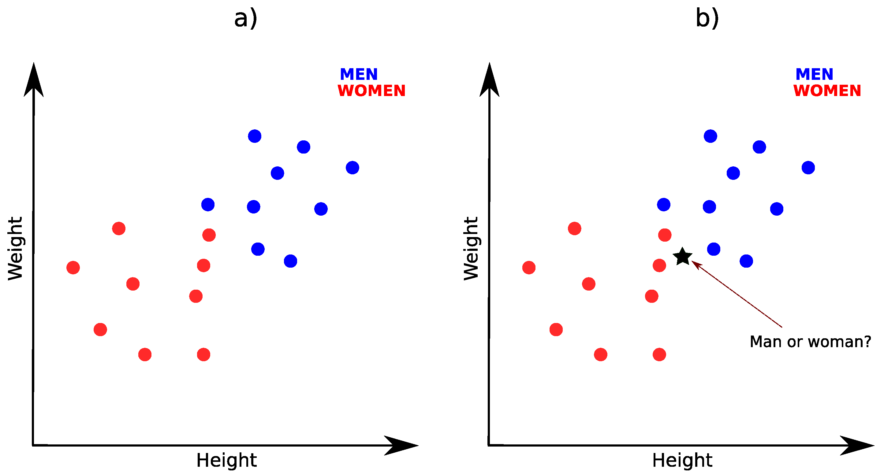
2.1. K-Nearest-Neighbors

K-Nearest-Neighbors or KNN is a simple classification algorithm first proposed by Evelyn Fix and Joseph Hodges [32] in 1951 and further developed by Thomas Cover [33] in 1967. This algorithm stores all the input data with its corresponding labels and classifies a new observation based on similarity [34]. This classification is done based on the labels of its nearest neighbors. The KNN algorithm has been used on several Industry 4.0 framework applications, such as cybersecurity [35], aircraft’s useful life prediction [36], fault classification [37], nephropathy prediction in children [38], intrusion detection systems [39], etc. In order to understand better how KNN works, let us take a brief example.

Data about the height and the weight of men and women were gathered and are presented in Figure 1a. The blue points represent data that were labeled as men and the red as women. Then, suppose that we add a new individual to the dataset. We are told that this new individual is a man; however, we only introduce their height and weight to the algorithm to see if it is capable of classifying them correctly. This is shown in Figure 1b, where the new individual is represented as a star.

To do the classification, we need to search for its nearest neighbors and their corresponding labels so that we can classify this new point depending on the majority of votes from its neighbors. To determine which of the data points are closest to the new observation, we have to measure the distance between data points.

There are several types of functions that can be used to obtain the distance between points, such as cosine similarity measure, Minkowsky, correlation, Chi-squared, and Euclidean distance [40]. From all of these, the most widely used function is the Euclidean distance, which is the measure of the straight line between two points and, for two dimensions, is obtained as:

$$d(x,y)=\sqrt{\sum _{i=1}^n{(x_i-y_i)}^2}$$

(1)

where d represents the distance between two points, and x and y represent the point coordinates. Once we obtain the distance between the new observation and the other points, we can choose the closest neighbors to proceed with the classification. However, an important question arises here: how many nearest neighbors should we consider? Let us take Figure 2 as an example.

In Figure 2, the new observation is being classified by its K nearest neighbors, where K has two different values: $K=3$ and $K=7$. For $K=3$, the closest neighbors are the ones inside the green circle, and for $K=7$, the closest neighbors are inside the purple circle. It can be seen that, if $K=3$, two of those three neighbors are women, so the new observation would be classified as a woman. However, if $K=7$, most of the closest neighbors are men, and then the new individual would be classified as a man. So, for the classification of this new individual, $K=7$ is better than $K=3$ because it classified it as a man, which was its real gender. Nevertheless, this does not mean that $K=7$ is the best overall value for the dataset; more new observations must be classified with different K values to find the value with the best performance.

As we can see, the resulting classification from the KNN algorithm strongly depends on the chosen number of nearest neighbors. Thus, the algorithm must be tested with different values of K until we find its most optimum value for the dataset that we are working with. This is usually the most time-demanding task when talking about the KNN algorithm. Once the optimum value of K is found, the training time is usually low, which is one of the main advantages when compared to other classification methods. Furthermore, another advantage of KNN is that it is very simple to implement and interpret, as was seen during the previous example. In addition, it is very useful when dealing with not linearly separable data and/or when there is no model that fits it well enough. Moreover, it is accurate for simple regression and classification tasks, so usually, it does not need to be compared with better-supervised learning models when dealing with this kind of problem. However, this algorithm also has some drawbacks, such as its accuracy depending on the data quality and being sensitive to irrelevant features. Furthermore, if there is a large quantity of data, the prediction time can be slower, turning it into a computationally expensive algorithm in some cases.

As a summary of the behavior of the KNN algorithm, we provide the pseudo-code shown in Algorithm 1, which is an interpretation of the algorithm developed by Fix, Hodges, and Cover [32,33].

Algorithm 1 KNN Pseudo-code

Input:    $x,l,s$ // $x:\mathrm{training}\mathrm{data}$; $l:\mathrm{label}$; $s:\mathrm{sample}\mathrm{to}\mathrm{classify}$ for i to training data size do:    Compute the distance $d(x_i,s)$ end for    Select the desired number k of nearest neighbors    Sort the distances by increasing order    Count the number of occurrences of each label among the top k neighbors Output: Assign to s the most frequent label l

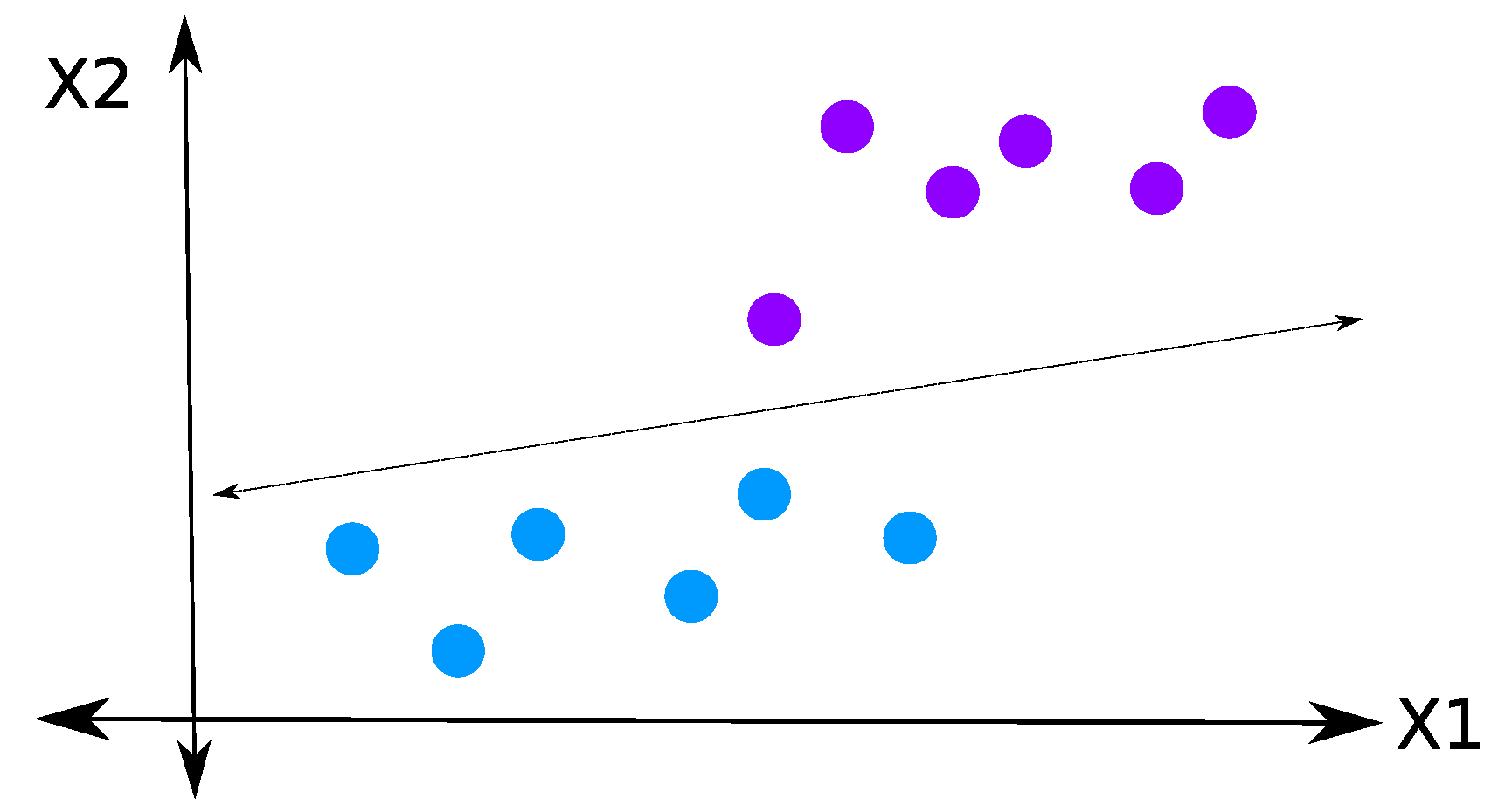
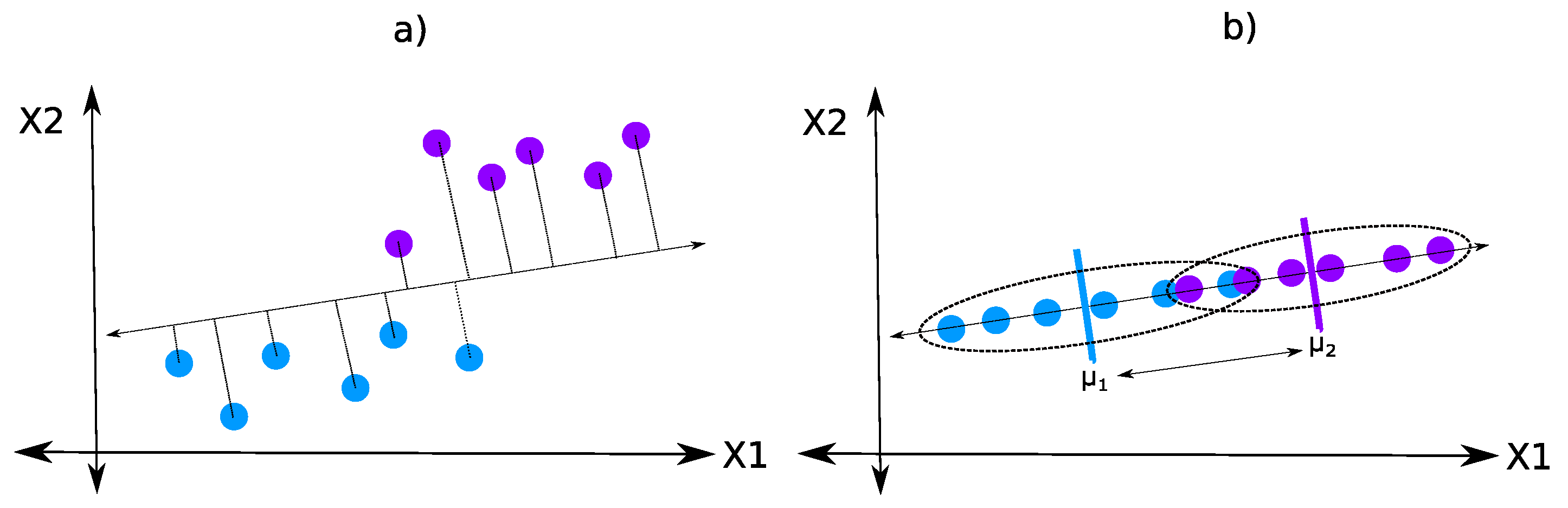
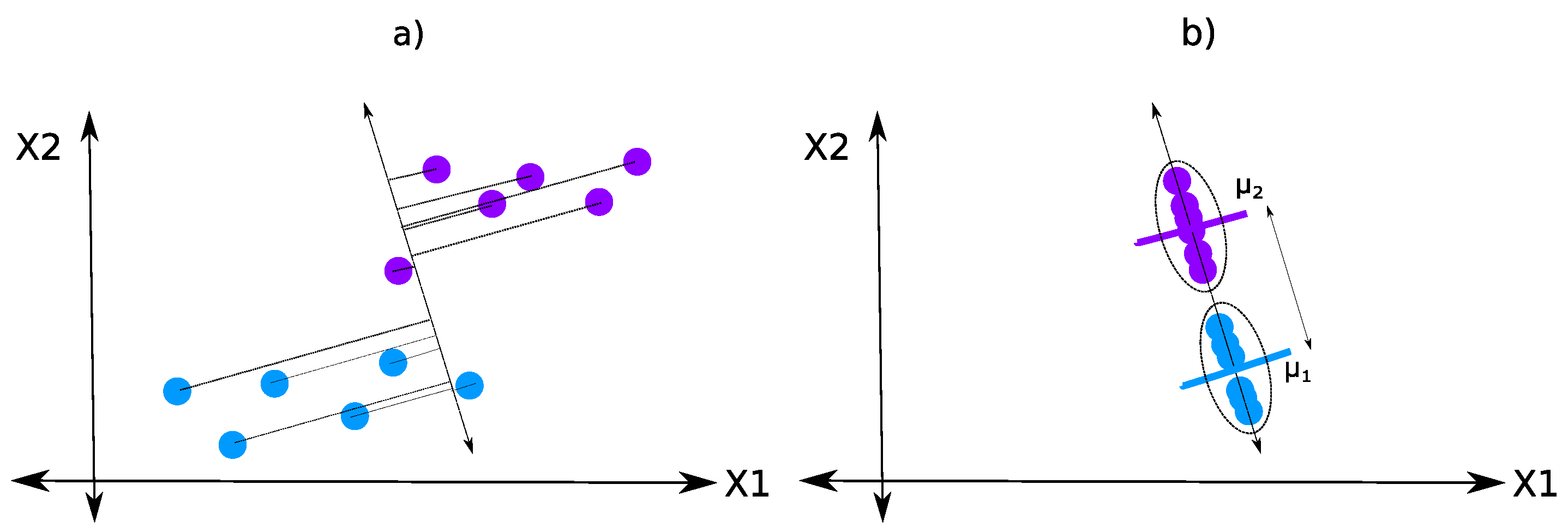
2.2. Linear Discriminant Analysis

Linear Discriminant Analysis or LDA, introduced by Ronald Fisher [41] in 1936, is a linear transformation algorithm used for dimensionality reduction and binary classification. The main objective of this algorithm is to project the data into a lower-dimensional space that maximizes the between-class variance while minimizing the within-class variance [42]. Some of the applications of LDA on Industry 4.0 include state of product detection [43], malfunction monitoring systems [44], EEG hand movement classification [45], etc. That being said, let us explore the theory behind LDA.

Let us suppose that we have one independent and one dependent variable, in which the latter is a binary one. The distribution of this variable with respect to the independent variable $X1$ is as follows:

In Figure 3, the blue and purple dots represent the different classes of the dependent variable. As we can see, it is not possible to divide these classes with a linear divider because they are scattered around the $X1$ axis. Then, we can conclude that a single independent variable is not enough to explain the behavior of our dependent variable. Hence, it may be a good idea to add a new explanatory variable $X2$ to our problem, as is shown in Figure 4.

Now, we can see that, with the new feature $X2$, it was easier to separate the blue and purple dots using a linear divider. However, this might not always be the case, and if we keep increasing the dimensional space, the problem may turn very complicated to deal with. In these cases, LDA becomes useful.

Linear Discriminant Analysis does an analysis over the entire feature space of the problem to create new axes in a lower-dimensional space. In the example we are dealing with, the two feature spaces can be reduced to a 1-D space using LDA to transform the original $X1$ and $X2$ axes to a new axis that ensures maximum between-class separability while minimizing within-class variance.

It is important to have in mind that both between-class and within-class variance are important for LDA to work correctly. This can be seen in Figure 5 and Figure 6, where Figure 5 only maximizes the between-class variance (arrow between means) while ignoring within-class variance (dotted ellipses), which leads to poor separation of classes. On the other hand, Figure 6 shows a new axis that maximizes between-class variance and minimizes within-class variance, leading to good class separation.

Now that we have a visual idea of how LDA works, let us explore the mathematics behind it. The general idea of LDA is to project a high-dimensional space into a line, and this projection must maximize the between-class variance and minimize the within-class variance. To find this projection, the linear discriminant finds a weight vector w that maximizes the Fisher’s criterion, defined as:

$$J\left(w\right)=\frac{{\left({\tilde{\mu }}_1-{\tilde{\mu }}_2\right)}^2}{{\tilde{S}}_1^2+{\tilde{S}}_2^2}$$

(2)

where $\widetilde{{\mu }_i}$ represents the means of projections of classes 1 and 2 ($\widetilde{{\mu }_i}=w^T{\mu }_i$), ${\mu }_i$ are the means of classes 1 and 2, and ${\tilde{S}}^2$ represents the variance (${\tilde{S}}_i^2={\sum }_{y_i\in {\mathrm{Class}}_i}{(y_i-{\tilde{\mu }}_i)}^2$), letting $y_i$ be the projected samples $y_i=w^T{x}_i$. Using these equalities, Fisher’s criterion can be written as a function of w as:

$$J\left(w\right)=\frac{w^T{S}_{B}w}{w^T{S}_{w}w}$$

(3)

where $S_B$ measures the separation between the means of two classes, and $S_w$ measures the within-class scattering. Then, given the previous equation, its maximum can be found by solving the generalized eigenvalue problem given by:

$$S_{B}w=\lambda S_{w}w$$

(4)

This will result in a set of eigenvectors w with eigenvalues $\lambda$. Finally, the eigenvectors are sorted from biggest to smallest depending on its eigenvalues, and a weight matrix W is created, which now represents the new space in which the data is projected.

In general, Linear Discriminant Analysis is a low computational cost classification method that is based on maximizing the distance between the means and minimizing within-class variance, making it simple to understand and implement. However, for it to work correctly we must have normally distributed data, which must also be linearly separable. Furthermore, this algorithm is only useful for binary classification problems and fails when the mean values are shared between both classes.

To be more explicit about the steps of the LDA algorithm, we provide the pseudo-code in Algorithm 2, which is based on the original Fisher’s proposal [41].

Algorithm 2 LDA Pseudo-code

Input:    $S=\left\{\left(x_1,y_1\right),\left(x_2,y_2\right),\dots ,\left(x_s,y_s\right)\right\}$ // $S:\mathrm{Training}\mathrm{set}$ Calculate:    The means $\mu$    Separations $S_B$ and $S_W$    Eigenvectors and eigenvalues: ($w_1,w_2,\dots ,w_n$),  (${\lambda }_1,{\lambda }_2,\dots ,{\lambda }_n$)    Sort the eigenvectors from biggest to smallest depending on the eigenvalues    Choose the top k eigenvectors    Produce matrix $W(n\times k)$ Output: Return matrix W

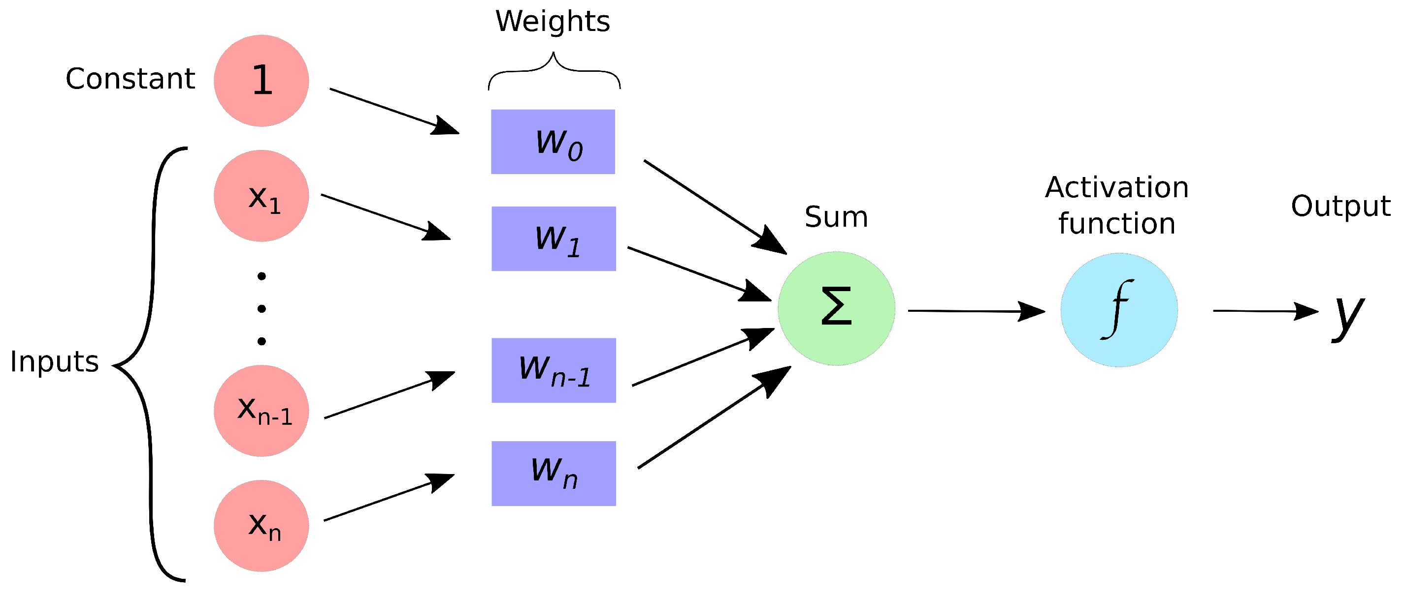
2.3. Simple Perceptron

The perceptron, first introduced by Rosenblatt [46], is the fundamental unit of artificial neural networks, just as the neuron is the fundamental unit of our central nervous system. Hence, it conforms the basis of advanced ML methods that are used on several real-life applications on Industry 4.0, such as smart manufacturing [47], condition monitoring [48], material selection [49], building occupancy prediction [50], among others. In the basic applications of Machine Learning, the Simple Perceptron is used as a supervised binary classifier [51], and it has four parts:

• Input
• Weights and bias
• Net sum
• Activation function

In Figure 7, it can be seen that one constant input is related to weight $w_0$. This weight is the bias ($-\theta$) of the system and represents the threshold that must be surpassed to fire the activation function. The system shown in Figure 7 can be mathematically represented as follows:

$$\begin{array}{cc}\hfill y& =1\mathrm{if}\sum _{i=0}^n{w}_i\times x_i\ge 0\hfill \\ \hfill & =0\mathrm{if}\sum _{i=0}^n{w}_i\times x_i<0\hfill \\ \hfill & \mathrm{where}{x}_0=1\mathrm{and}{w}_0=-\theta \hfill \end{array}$$

(5)

As we can see, the perceptron has two possible outcomes, and the outcome changes from 0 (negative) to 1 (positive) if the weighted sum of the inputs surpasses the threshold $\theta$. This weighted sum depends directly on the weight vector (w) of the system, and the goal of training the perceptron is to find vector w, which allows us to correctly classify our negative and positive inputs.

Vector w is randomly initialized, and then it is tuned depending on the behavior of the system. We know that if an input $x_n$ has a positive label, the dot product between the weight vector and the input vector (x) must be greater or equal than 0, and if the label is negative, the dot product must be lower than 0. Knowing this, there can be two cases of misclassification. These cases are shown below with their corresponding corrective action:

• The input label is negative, and the dot product is greater or equal than 0. When this is the case, we must update w by subtracting the input vector to the weight vector.
• The input label is positive, and the dot product is lower than 0. When this happens, we must update w by adding the input vector to the weight vector.

Based on the method’s description, we can see that the single perceptron is easy to set up, train, and implement. Furthermore, depending on which is the activation function, we can allow the algorithm to be linked to posterior probabilities, an example of this can be seen while using the sigmoid function. On the other hand, this algorithm is limited to work on linearly separable data, and thus, it can only create hyperplane threshold boundaries. Finally, for ease of understanding, we provide the pseudo-code in Algorithm 3, which summarizes the method originally provided by Rosenblatt [46].

Algorithm 3 Simple Perceptron Pseudo-code

Input:    Vector x    Label 0 = Negative (N) input    Label 1 = Positive (P) input Training:    Randomly initialize w misclassification != 0 $x\in N\mathrm{and}{\sum }_{i=0}^n{w}_i\times x_i\ge 0$ w = w − x $x\in P\mathrm{and}{\sum }_{i=0}^n{w}_i\times x_i<0$ w = w + x Output: Parameters w

3. Advantages and Disadvantages of the Methods

It is intended to test the behavior of each of the previously described methods for a set of case studies. However, before doing that, we should clarify the advantages and disadvantages of each method, which are shown in

Table 1. Advantages and disadvantages of the methods.

Method	Advantages	Disadvantages	Ref
KNN	- Easy to understand and implement - Fast training - Robust to noisy traning data - Good behaviour dealing with several labels	- High computational cost - Poor run time performance - Sensitive to local structure of the data	[52,53]
LDA	- Low computational cost - Easy to implement - Discriminate different groups - Visual representation makes clear understanding	- Requires normal distribution - Linear decision boundaries - Limited to two classes	[54,55]
Perceptron	- Easy training and set up - Yields the decision function directly through training	- Only works on linearly separable data - Boundaries are only allowed to be hyperplanes - Limited to binary data	[56]

.

4. Case Studies

As mentioned earlier, one of the main pillars of Education 4.0 is not only to teach students the theory behind disruptive technologies, such as ML, but also to provide the learning material so that they can have the opportunity of applying the acquired knowledge to develop problem-solving skills, as well competencies such as design mindset, transdisciplinary approach and computational skills [3]. Thus, the previous ML algorithms were applied over three different datasets while showing and analyzing the results so that they can be employed by students to learn more about their application.

Moreover, providing this test bench is not only useful for students but also for teachers as support material on Machine Learning lessons. For example, it can be used as a project in which students must replicate the results presented here so that they can develop computational skills over ML problems. Furthermore, teachers can entrust students to design their own experiment so that they apply the methods on a different dataset of their choice to see how it works, compare the obtained performance, and analyze why they were good or bad classifiers for the proposed new dataset.

For this work, the proposed test bench consists of the following three datasets: the Cleveland Clinic Foundation Heart Disease dataset, the Banknote Authentication dataset, and the Breast Cancer Wisconsin dataset, which are available at the UCI Machine Learning Repository. These datasets were chosen to be about medicine and economics for students to notice that the applications of ML are multidisciplinary and not limited to engineering problems.

The former dataset contains the data of 296 patients, which is composed of 14 attributes per patient, including the classification of each of them. There are two categories in which the patients are classified: healthy patients and heart disease patients. The second dataset contains 1372 items with four attributes, where each item is labeled as genuine or fake depending on its attributes. Finally, the Wisconsin dataset has 30 features for each of the 569 instances, where each instance is classified as malignant or benign. Prior to the implementation of the classification algorithms, the datasets were standardized.

4.1. Method

To estimate the performance of KNN, LDA, and Perceptron, we used repeated k-fold cross-validation, with $k=5$ and 100 repetitions for each algorithm. For the KNN algorithm, a number of 23 close neighbors was found to be the best choice for the Cleveland dataset, while for Banknote and Wisconsin datasets, 4 and 5 close neighbors were the best choices, respectively.

We evaluated if the data was correctly classified based on the number of true positives ($TP$), false negatives ($FN$), false positives ($FP$), and true negatives ($TN$). The accuracy and error of each system are then defined as:

$$Acc=\frac{TP+FN}{TP+TN+FP+FN}$$

(6)

$$error=Acc=\frac{FP+FN}{TP+TN+FP+FN}=1-Acc$$

(7)

Other metrics that were used to evaluate the performance of the algorithms were:

• Sensitivity ($TPR$): represents the probability of detecting the condition when it is present. $TPR=\frac{TP}{TP+FN}$
• False negative rate ($FNR$): represents the probability of not detecting the condition when it is present. $FNR=\frac{FN}{TP+FN}$
• False positive rate ($FPR$): represents the probability of detecting the condition when it is not present. $FPR=\frac{FP}{TN+FP}$
• Specificity ($TNR$): represents the probability of not detecting the condition when it is not present. $TNR=\frac{TN}{TN+FP}$
• Positive predictive value ($PPV$): represents the probability of the patient really having the condition when the test is positive. $PPV=\frac{TP}{TP+FP}$
• Negative predictive value ($NPV$): represents the probability of the patient not having the condition when the test is negative. $NPV=\frac{TN}{TN+FN}$

Apart from these metrics, the area under the ROC curve was also used to evaluate the performance of the algorithms. Furthermore, a MANOVA analysis was carried out to see if there was any statistical difference between the algorithms ($p=0.05$).

4.2. Results

For each of the previous metrics, KNN, LDA, and Simple Perceptron obtained the mean values shown in

Table 2. The mean value for each metric for each algorithm—Cleveland Heart Disease dataset.

Algorithm	Metrics
	AUC	ACC	TPR	FNR	FPR	TNR	PPV	NPV
KNN	0.9025	0.8342	0.8168	0.1831	0.1394	0.8606	0.8928	0.7684
LDA	0.9023	0.8349	0.8266	0.1734	0.1522	0.8477	0.8776	0.7864
Perceptron	0.8481	0.7840	0.8265	0.7812	0.2187	0.7407	0.7815	0.7407

,

Table 3. The mean value for each metric for each algorithm—Banknote Authentication dataset.

Algorithm	Metrics
	AUC	ACC	TPR	FNR	FPR	TNR	PPV	NPV
KNN	0.9987	0.9985	1.0000	0.0000	0.0033	0.9967	0.9973	1.0000
LDA	0.9996	0.9762	0.9999	0.0001	0.0506	0.9494	0.9574	0.9999
Perceptron	0.9986	0.9805	1.0000	0.0000	0.0370	0.9629	0.9653	1.0000

and

Table 4. The mean value for each metric for each algorithm—Breast Cancer Wisconsin dataset.

Algorithm	Metrics
	AUC	ACC	TPR	FNR	FPR	TNR	PPV	NPV
KNN	0.9862	0.9657	0.9807	0.0193	0.0423	0.9577	0.9266	0.9890
LDA	0.9908	0.9564	0.9903	0.0096	0.0608	0.9392	0.8919	0.9949
Perceptron	0.9901	0.9663	1.0000	0.0000	0.0800	0.9200	0.8636	1.0000

. Analyzing them, we can observe that for the Cleveland dataset, the KNN algorithm showed the best behavior for AUC, FPR, TNR, and PPV; for the other metrics, the best algorithm was LDA. For the Banknote dataset, KNN was the best classifier for almost all the metrics, except AUC, where LDA had the best result. Finally, for the Wisconsin dataset, Perceptron outperformed the other two algorithms on ACC, TPR, FNR, and NPV, while LDA had the best performance for AUC and KNN for FPR, TNR, and PPV.

Apart from this, the MANOVA test showed that there was an overall statistical difference between the algorithms applied on this test bench for a p-value of $p=0.05$. However, a post hoc Tukey test was carried out to identify the specific differences between the algorithms. This test showed that for the Cleveland dataset, the KNN and LDA algorithms do not differ significantly for most of the parameters, except for PPV and NPV. In comparison to the Simple Perceptron, these two algorithms were confirmed to be significantly different. For the Banknote dataset, the Tukey test showed that there was no statistical difference between the three algorithms on the TPR, FNR, and NPV parameters; moreover, KNN and Simple Perceptron were also no statistically different in their accuracy value. Finally, for the Wisconsin dataset, we found that KNN and Perceptron were not statistically different over ACC and AUC, while LDA and Simple Perceptron were also not different in their AUC value.

5. Final Remarks

Machine learning applications are rapidly increasing in Industry 4.0 development; thus, it is important for students to learn at least the basics of some ML algorithms. Therefore, Education 4.0 is in charge of introducing future professionals to this area, as well as providing them with the possibility of testing their understanding in real-life scenarios. Hence, the primary objective of this work was to give the students an introduction to Machine Learning and three different classification (supervised) algorithms: K-Nearest-Neighbor, Linear Discriminant Analysis, and Simple Perceptron.

This introduction was done through a brief review of the methods, their pseudo-codes, as well as a comparison between them. Through this comparison students can observe that, despite the three methods being able to classify data, LDA and perceptron are only able to deal with binary data, meaning that they are not useful for multi-class classification. Moreover, it is important for students to notice that KNN is able to classify data in any desired number of classes; however, unlike the other two algorithms, this method usually has a high computational cost that increases proportionally to the number of classes and data size. Furthermore, one of the main differences for students to remember between KNN and the other two methods is that the former is able to deal with not-linearly separable data, while the last ones cannot be used for this kind of problem. Furthermore, the only algorithm that has the capacity of giving us the posterior classification probabilities of the input data is the Simple Perceptron, being one of the main advantages of this method when compared to KNN and LDA. Finally, among the three methods, we recall students that the easiest to understand and implement is KNN, followed by Simple Perceptron, and finally LDA.

Furthermore, in order to contribute to the development of new and updated educational material that is useful for teachers and students under the Education 4.0 framework, we developed a multidisciplinary test bench by applying these supervised algorithms over the Cleveland Heart Disease dataset, Banknote Authentication dataset, and Wisconsin Breast Cancer dataset to explore their behavior. From the obtained results, students can notice that, for the proposed metrics and datasets, the overall best performance was achieved from the KNN algorithm, followed by LDA and then Simple Perceptron. Furthermore, using MANOVA and Tuckey tests, it can be observed for which parameters the algorithms were statistically different over the presented test bench.

Through the previous description of the algorithms and the results of their application over the proposed test-bench, this study provides students with the possibility of learning the basic theory of KNN, LDA, and Simple Perceptron, as well as serving as a guide for the practical application of the acquired knowledge towards the solution real-life problems. Moreover, teachers that are dabbling into the Education 4.0 framework can use this material to introduce their students to Machine Learning theory and applications. Furthermore, it can also be used as an additional reading/exercise that reinforces the understanding of the student posterior to a Machine Learning lesson.

Despite offering students the possibility of learning through this test bench and developing skills such as design mindset, transdisciplinary approach, and computational skills, the work and learning process is not limited to the presented datasets. One idea for teachers to test and validate the knowledge and skills and to further enhance the competencies that students can acquire through the content of this paper is to propose a Project-Based Learning (PBL) homework, where students replicate the results shown in this work and then search for other real-life datasets that could be analyzed with the presented algorithms. Through this PBL proposal, they can test how well they understood the presented information while gaining more knowledge and skills through research and further application of the methods.

Regardless of the contribution of this study to the Education 4.0 framework, the work is not over. Further research can be done in order to provide students and teachers with more ML educational material that covers additional algorithms that can be used to solve Industry 4.0 problems such as Random Forest, Naive-Bayes, K-means, Support Vector Machines, Artificial Neural Networks, etc. Additionally, an improved test bench, with a broader amount of transdisciplinary datasets, may also be a way to enhance the student’s comprehension of these topics.

References

1. Xu, L.D.; Xu, E.L.; Li, L. Industry 4.0: State of the art and future trends. Int. J. Prod. Res. 2018, 56, 2941–2962. [Google Scholar] [CrossRef] [Green Version]
2. Rodríguez-Abitia, G.; Bribiesca-Correa, G. Assessing Digital Transformation in Universities. Future Internet 2021, 13, 52. [Google Scholar] [CrossRef]
3. Ramirez-Mendoza, R.A.; Morales-Menendez, R.; Iqbal, H.; Parra-Saldivar, R. Engineering Education 4.0: Proposal for a new Curricula. In Proceedings of the 2018 IEEE Global Engineering Education Conference (EDUCON), Santa Cruz de Tenerife, Spain, 17–20 April 2018; pp. 1273–1282. [Google Scholar]
4. Karacay, G. Talent development for Industry 4.0. In Industry 4.0: Managing the Digital Transformation; Springer: Berlin/Heidelberg, Germany, 2018; pp. 123–136. [Google Scholar]
5. Quintana, C.D.D.; Mora, J.G.; Pérez, P.J.; Vila, L.E. Enhancing the development of competencies: The role of UBC. Eur. J. Educ. 2016, 51, 10–24. [Google Scholar] [CrossRef] [Green Version]
6. Prieto, M.D.; Sobrino, Á.F.; Soto, L.R.; Romero, D.; Biosca, P.F.; Martínez, L.R. Active learning based laboratory towards engineering education 4.0. In Proceedings of the 2019 24th IEEE International Conference on Emerging Technologies and Factory Automation (ETFA), Zaragoza, Spain, 10–13 September 2019; pp. 776–783. [Google Scholar]
7. Zhang, X.D. A Matrix Algebra Approach to Artificial Intelligence; Springer: Berlin/Heidelberg, Germany, 2020. [Google Scholar]
8. Ahmad, M.A.; Eckert, C.; Teredesai, A. Interpretable machine learning in healthcare. In Proceedings of the 2018 ACM International Conference on Bioinformatics, Computational Biology, and Health Informatics, Washington, DC, USA, 29 August–1 September 2018; pp. 559–560. [Google Scholar]
9. Parthiban, G.; Srivatsa, S. Applying machine learning methods in diagnosing heart disease for diabetic patients. Int. J. Appl. Inf. Syst. (IJAIS) 2012, 3, 25–30. [Google Scholar] [CrossRef]
10. Iyer, A.; Jeyalatha, S.; Sumbaly, R. Diagnosis of diabetes using classification mining techniques. arXiv 2015, arXiv:1502.03774. [Google Scholar] [CrossRef]
11. Sen, S.K.; Dash, S. Application of meta learning algorithms for the prediction of diabetes disease. Int. J. Adv. Res. Comput. Sci. Manag. Stud. 2014, 2, 396–401. [Google Scholar]
12. Senturk, Z.K.; Kara, R. Breast cancer diagnosis via data mining: Performance analysis of seven different algorithms. Comput. Sci. Eng. 2014, 4, 35. [Google Scholar] [CrossRef]
13. Williams, K.; Idowu, P.A.; Balogun, J.A.; Oluwaranti, A.I. Breast cancer risk prediction using data mining classification techniques. Trans. Netw. Commun. 2015, 3, 1. [Google Scholar] [CrossRef]
14. Papageorgiou, E.I.; Papandrianos, N.I.; Apostolopoulos, D.J.; Vassilakos, P.J. Fuzzy cognitive map based decision support system for thyroid diagnosis management. In Proceedings of the 2008 IEEE International Conference on Fuzzy Systems (IEEE World Congress on Computational Intelligence), Hong Kong, China, 1–6 June 2008; pp. 1204–1211. [Google Scholar]
15. Zhu, W.; Liu, C.; Fan, W.; Xie, X. Deeplung: Deep 3d dual path nets for automated pulmonary nodule detection and classification. In Proceedings of the 2018 IEEE Winter Conference on Applications of Computer Vision (WACV), Lake Tahoe, NV, USA, 12–15 March 2018; pp. 673–681. [Google Scholar]
16. Afshar, P.; Mohammadi, A.; Plataniotis, K.N. Brain tumor type classification via capsule networks. In Proceedings of the 2018 25th IEEE International Conference on Image Processing (ICIP), Athens, Greece, 7–10 October 2018; pp. 3129–3133. [Google Scholar]
17. Heaton, J.B.; Polson, N.G.; Witte, J.H. Deep learning for finance: Deep portfolios. Appl. Stoch. Model. Bus. Ind. 2017, 33, 3–12. [Google Scholar] [CrossRef]
18. De Prado, M.L. Building diversified portfolios that outperform out of sample. J. Portf. Manag. 2016, 42, 59–69. [Google Scholar] [CrossRef]
19. Raffinot, T. Hierarchical clustering-based asset allocation. J. Portf. Manag. 2017, 44, 89–99. [Google Scholar] [CrossRef]
20. Cao, L.J.; Tay, F.E.H. Support vector machine with adaptive parameters in financial time series forecasting. IEEE Trans. Neural Netw. 2003, 14, 1506–1518. [Google Scholar] [CrossRef] [Green Version]
21. Fan, A.; Palaniswami, M. Stock selection using support vector machines. In Proceedings of the IJCNN’01. International Joint Conference on Neural Networks. Proceedings (Cat. No. 01CH37222), Washington, DC, USA, 15–19 July 2001; Volume 3, pp. 1793–1798. [Google Scholar]
22. Nayak, R.K.; Mishra, D.; Rath, A.K. A Naïve SVM-KNN based stock market trend reversal analysis for Indian benchmark indices. Appl. Soft Comput. 2015, 35, 670–680. [Google Scholar] [CrossRef]
23. Zhang, X.D.; Li, A.; Pan, R. Stock trend prediction based on a new status box method and AdaBoost probabilistic support vector machine. Appl. Soft Comput. 2016, 49, 385–398. [Google Scholar] [CrossRef]
24. Anifowose, F.A.; Labadin, J.; Abdulraheem, A. Ensemble machine learning: An untapped modeling paradigm for petroleum reservoir characterization. J. Pet. Sci. Eng. 2017, 151, 480–487. [Google Scholar] [CrossRef]
25. Voyant, C.; Notton, G.; Kalogirou, S.; Nivet, M.L.; Paoli, C.; Motte, F.; Fouilloy, A. Machine learning methods for solar radiation forecasting: A review. Renew. Energy 2017, 105, 569–582. [Google Scholar] [CrossRef]
26. Heinermann, J.; Kramer, O. Machine learning ensembles for wind power prediction. Renew. Energy 2016, 89, 671–679. [Google Scholar] [CrossRef]
27. Zeng, Y.R.; Zeng, Y.; Choi, B.; Wang, L. Multifactor-influenced energy consumption forecasting using enhanced back-propagation neural network. Energy 2017, 127, 381–396. [Google Scholar] [CrossRef]
28. Zeng, Y.; Liu, J.; Sun, K.; Hu, L.W. Machine learning based system performance prediction model for reactor control. Ann. Nucl. Energy 2018, 113, 270–278. [Google Scholar] [CrossRef]
29. Evans, J.; Jones, R.; Karvonen, A.; Millard, L.; Wendler, J. Living labs and co-production: University campuses as platforms for sustainability science. Curr. Opin. Environ. Sustain. 2015, 16, 1–6. [Google Scholar] [CrossRef]
30. Detrano, R. The Cleveland Heart Disease Data Set; VA Medical Center, Long Beach and Cleveland Clinic Foundation: Long Beach, CA, USA, 1988. [Google Scholar]
31. Dua, D.; Graff, C. UCI Machine Learning Repository; University of California: Irvine, CA, USA, 2017. [Google Scholar]
32. Evelyn, F.; Hodges, J. Discriminatory Analysis-Nonparametric Discrimination: Consistency Properties; Technical Report; International Statistical Institute (ISI): Voorburg, The Netherlands, 1989; pp. 238–247. [Google Scholar]
33. Cover, T.; Hart, P. Nearest neighbor pattern classification. IEEE Trans. Inf. Theory 1967, 13, 21–27. [Google Scholar] [CrossRef]
34. Sun, S.; Huang, R. An adaptive k-nearest neighbor algorithm. In Proceedings of the 2010 Seventh International Conference on Fuzzy Systems and Knowledge Discovery, Yantai, China, 10–12 August 2010; Volume 1, pp. 91–94. [Google Scholar]
35. Romeo, L.; Loncarski, J.; Paolanti, M.; Bocchini, G.; Mancini, A.; Frontoni, E. Machine learning-based design support system for the prediction of heterogeneous machine parameters in industry 4.0. Expert Syst. Appl. 2020, 140, 112869. [Google Scholar] [CrossRef]
36. Taha, H.A.; Sakr, A.H.; Yacout, S. Aircraft Engine Remaining Useful Life Prediction Framework for Industry 4.0. In Proceedings of the 4th North America conference on Industrial Engineering and Operations Management, Toronto, ON, Canada, 23–25 October 2019. [Google Scholar]
37. Zhou, C.; Tham, C.K. Graphel: A graph-based ensemble learning method for distributed diagnostics and prognostics in the industrial internet of things. In Proceedings of the 2018 IEEE 24th International Conference on Parallel and Distributed Systems (ICPADS), Singapore, 11–13 December 2018; pp. 903–909. [Google Scholar]
38. Zhang, P.; Wang, R.; Shi, N. IgA Nephropathy Prediction in Children with Machine Learning Algorithms. Future Internet 2020, 12, 230. [Google Scholar] [CrossRef]
39. Thapa, N.; Liu, Z.; Kc, D.B.; Gokaraju, B.; Roy, K. Comparison of machine learning and deep learning models for network intrusion detection systems. Future Internet 2020, 12, 167. [Google Scholar] [CrossRef]
40. Hu, L.Y.; Huang, M.W.; Ke, S.W.; Tsai, C.F. The distance function effect on k-nearest neighbor classification for medical datasets. SpringerPlus 2016, 5, 1–9. [Google Scholar] [CrossRef] [Green Version]
41. Fisher, R.A. The use of multiple measurements in taxonomic problems. Ann. Eugen. 1936, 7, 179–188. [Google Scholar] [CrossRef]
42. Xanthopoulos, P.; Pardalos, P.M.; Trafalis, T.B. Linear discriminant analysis. In Robust Data Mining; Springer: Berlin/Heidelberg, Germany, 2013; pp. 27–33. [Google Scholar]
43. Kuo, C.J.; Ting, K.C.; Chen, Y.C. State of product detection method applicable to Industry 4.0 manufacturing models with small quantities and great variety: An example with springs. In Proceedings of the 2017 International Conference on Applied System Innovation (ICASI), Sapporo, Japan, 13–17 May 2017; pp. 1650–1653. [Google Scholar]
44. Natesha, B.; Guddeti, R.M.R. Fog-based Intelligent Machine Malfunction Monitoring System for Industry 4.0. IEEE Trans. Ind. Inform. 2021. [Google Scholar] [CrossRef]
45. Bressan, G.; Cisotto, G.; Müller-Putz, G.R.; Wriessnegger, S.C. Deep learning-based classification of fine hand movements from low frequency EEG. Future Internet 2021, 13, 103. [Google Scholar] [CrossRef]
46. Rosenblatt, F. The Perceptron, a Perceiving and Recognizing Automaton Project Para; Cornell Aeronautical Laboratory: Buffalo, NY, USA, 1957. [Google Scholar]
47. Matheri, A.N.; Ntuli, F.; Ngila, J.C.; Seodigeng, T.; Zvinowanda, C. Performance prediction of trace metals and cod in wastewater treatment using artificial neural network. Comput. Chem. Eng. 2021, 149, 107308. [Google Scholar] [CrossRef]
48. Żabiński, T.; Mączka, T.; Kluska, J.; Madera, M.; Sęp, J. Condition monitoring in Industry 4.0 production systems-the idea of computational intelligence methods application. Procedia CIRP 2019, 79, 63–67. [Google Scholar] [CrossRef]
49. Merayo, D.; Rodriguez-Prieto, A.; Camacho, A. Comparative analysis of artificial intelligence techniques for material selection applied to manufacturing in Industry 4.0. Procedia Manuf. 2019, 41, 42–49. [Google Scholar] [CrossRef]
50. Hitimana, E.; Bajpai, G.; Musabe, R.; Sibomana, L.; Kayalvizhi, J. Implementation of IoT Framework with Data Analysis Using Deep Learning Methods for Occupancy Prediction in a Building. Future Internet 2021, 13, 67. [Google Scholar] [CrossRef]
51. Sagheer, A.; Zidan, M.; Abdelsamea, M.M. A novel autonomous perceptron model for pattern classification applications. Entropy 2019, 21, 763. [Google Scholar] [CrossRef] [PubMed] [Green Version]
52. Jadhav, S.D.; Channe, H. Comparative study of K-NN, naive Bayes and decision tree classification techniques. Int. J. Sci. Res. (IJSR) 2016, 5, 1842–1845. [Google Scholar]
53. De Leonardis, G.; Rosati, S.; Balestra, G.; Agostini, V.; Panero, E.; Gastaldi, L.; Knaflitz, M. Human Activity Recognition by Wearable Sensors: Comparison of different classifiers for real-time applications. In Proceedings of the 2018 IEEE International Symposium on Medical Measurements and Applications (MeMeA), Rome, Italy, 11–13 June 2018; pp. 1–6. [Google Scholar]
54. Lakshmi, M.R.; Prasad, T.; Prakash, D.V.C. Survey on EEG signal processing methods. Int. J. Adv. Res. Comput. Sci. Softw. Eng. 2014, 4, 84–91. [Google Scholar]
55. Mahmood, S.H.; Khidir, H.H. Using Discriminant Analysis for Classification of Patient Status after Three Months from Brain Stroke. Zanco J. Humanit. Sci. 2020, 24, 206–223. [Google Scholar]
56. Park, Y.S.; Lek, S. Artificial neural networks: Multilayer perceptron for ecological modeling. In Developments in Environmental Modelling; Elsevier: Amsterdam, The Netherlands, 2016; Volume 28, pp. 123–140. [Google Scholar]
Figure 1. (a) Men and women distribution according to height and weight. (b) New observation added to the dataset.
Futureinternet 13 00193 g001
Figure 2. Classification based on different values of K.
Futureinternet 13 00193 g002
Figure 3. The distribution of dependent variables.
Futureinternet 13 00193 g003
Figure 4. The 2-D distribution of dependent variables.
Futureinternet 13 00193 g004
Figure 5. (a) The projection of data points on a new “bad” axis. (b) The resultant separation with the new axis.
Futureinternet 13 00193 g005
Figure 6. (a) The projection of data points on a new “good” axis. (b) The resultant separation with the new axis.
Futureinternet 13 00193 g006
Figure 7. The Perceptron model.
Futureinternet 13 00193 g007