Article

An Efficient Deep Convolutional Neural Network Approach for Object Detection and Recognition Using a Multi-Scale Anchor Box in Real-Time

by
Vijayakumar Varadarajan
1,*,
Dweepna Garg
2 and
Ketan Kotecha
3
1
School of Computer Science and Engineering, The University of New South Wales, Sydney 1466, Australia
2
Department of Computer Engineering, Devang Patel Institute of Advance Technology and Research (DEPSTAR), Faculty of Technology and Engineering (FTE), Charotar University of Science and Technology (CHARUSAT), Anand 388421, India
3
Symbiosis Centre for Applied Artificial Intelligence, Symbiosis International (Deemed University), Pune 412115, India
*
Author to whom correspondence should be addressed.
Future Internet 2021, 13(12), 307; https://doi.org/10.3390/fi13120307
Submission received: 21 October 2021 / Revised: 24 November 2021 / Accepted: 26 November 2021 / Published: 29 November 2021
(This article belongs to the Special Issue Big Data Analytics, Privacy and Visualization)

Abstract

:
Deep learning is a relatively new branch of machine learning in which computers are taught to recognize patterns in massive volumes of data. It primarily describes learning at various levels of representation, which aids in understanding data that includes text, voice, and visuals. Convolutional neural networks have been used to solve challenges in computer vision, including object identification, image classification, semantic segmentation and a lot more. Object detection in videos involves confirming the presence of the object in the image or video and then locating it accurately for recognition. In the video, modelling techniques suffer from high computation and memory costs, which may decrease performance measures such as accuracy and efficiency to identify the object accurately in real-time. The current object detection technique based on a deep convolution neural network requires executing multilevel convolution and pooling operations on the entire image to extract deep semantic properties from it. For large objects, detection models can provide superior results; however, those models fail to detect the varying size of the objects that have low resolution and are greatly influenced by noise because the features after the repeated convolution operations of existing models do not fully represent the essential characteristics of the objects in real-time. With the help of a multi-scale anchor box, the proposed approach reported in this paper enhances the detection accuracy by extracting features at multiple convolution levels of the object. The major contribution of this paper is to design a model to understand better the parameters and the hyper-parameters which affect the detection and the recognition of objects of varying sizes and shapes, and to achieve real-time object detection and recognition speeds by improving accuracy. The proposed model has achieved 84.49 mAP on the test set of the Pascal VOC-2007 dataset at 11 FPS, which is comparatively better than other real-time object detection models.

1. Introduction and Scope

Computer vision is a very sophisticated branch of artificial intelligence that focuses on the imitation of the human visual system. With the help of computer vision, the computer first identifies and then processes the objects which are present in images and videos. With the advancement in machine learning and deep learning, the field can perform just as well as humans in some of the tasks like detecting and labelling objects. The driving factor for the increased growth of computer vision is the huge amount of data generated, which is being used to train and make computer vision better. Deep learning is considered to be one of the effective methods for carrying out computer vision. A good deep learning algorithm considers a huge number of trained datasets, and the parameters can be tuned to re-train the model for various other applications. Here, the term parameters include: the number of hidden layers, type of layers, training epochs, and many more. Deep learning has revolutionized the developments in image processing, natural language processing, biology, autonomous driving, artificial intelligence, and more [1]. Deep learning is regarded as the subset of machine learning that uses a hierarchical level of layers to carry out machine learning [2]. Traditionally, data analysis was performed linearly; however, with the advent of deep learning, machines can now process data in a nonlinear approach [3].
This paper focuses on object detection and recognition. The challenging task at the initial stage is to distinguish between the related computer vision tasks. For example, it might be difficult to differentiate between image classifications, object localization, and object detection. Object detection involves both a bounding box around an image and assigning a class label. Altogether it is referred to as object recognition. The past work that has been undertaken regarding object detection involves the extraction of the features by using algorithms like HOG [4], SIFT [5], and SURF [6]. These algorithms use the traditional machine learning approaches, i.e., first performing feature extraction and then training the algorithm to achieve the desired output; however, deep learning algorithms have shown a significant advantage over the traditional machine learning approach by training the algorithm from the data itself. No features are extracted manually. The deep learning algorithm differs as in it a network is used to extract features along with bounding box prediction, etc. As a result of this, a faster and more accurate object detection system is obtained. This paper deals with the deep convolutional neural network model for efficiently detecting and recognizing the varying sizes of objects from a video sequence.
The existing detection models were successful in achieving better results for large-sized objects. On the other hand, the existing models fail to detect small objects with poor resolution and are strongly influenced by noise because the features of existing models after multiple convolution procedures do not accurately capture the core characteristics of small objects. A comparison of the proposed algorithm with the existing methods was also carried out by considering various parameters like accuracy, frames per second, epochs, dropout, learning rate, resolution, precision, and recall. The scope of our work is limited to the Pascal VOC dataset [7].

1.1. Contributions

In summary the main contribution of this work is:
(1)
Design and implementation of the model for accurate detection and recognition of objects from a video sequence.
(2)
Design a model to understand better the parameters and the hyper-parameters which affect the detection and the recognition of objects of varying sizes and shapes.
(3)
Achieve real-time object detection and recognition speeds by improving accuracy.
(4)
Develop implementations to take full advantage of the GPU implementations.

1.2. Novelty

(1)
Experimentation to detect objects of varying sizes from a video sequence.
(2)
Comparison of the existing work with the proposed model.
(3)
Generation of a multi-scale anchor box to obtain better results.
(4)
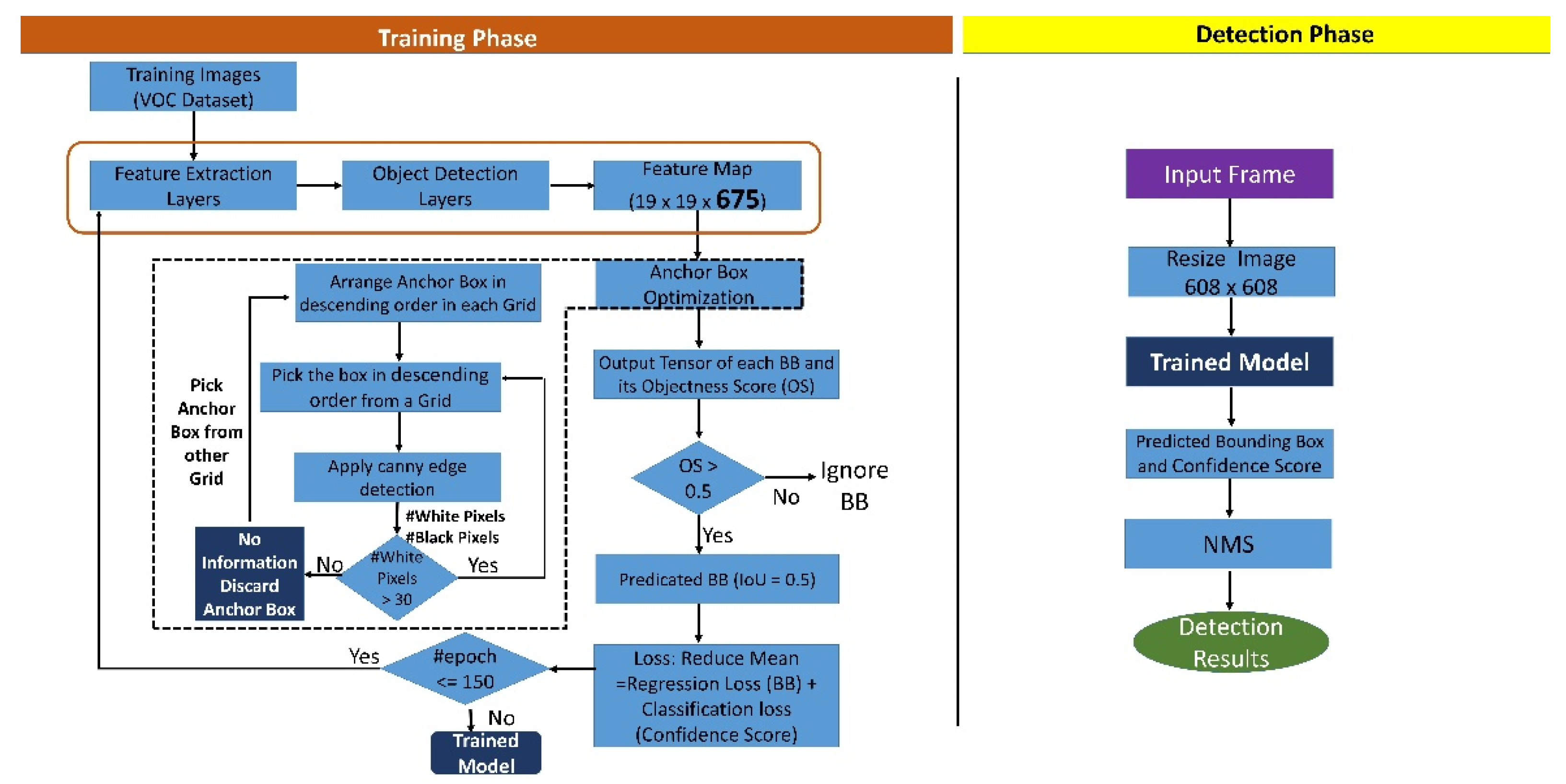
Concept of an efficient multi-scale anchor box approach is used in the proposed work to obtain better results by arranging the anchor boxes in descending order (i.e., large scale anchor box first and then moving towards small sized anchor box). If the information is not present in the large-scale anchor box, there is no need to move for a small-scale anchor box. This saves execution time for each time predicting the prediction score of the information present in the given anchor box because it reduces the search space for object recognition.

1.3. Outline

The paper is organized as follows: Section 2 presents the background study followed by Section 3 which describes the methods of the architecture employed in detail. Section 4 presents the experimentation, evaluations and results. Section 5 concludes the paper with an overview and future work.

2. Background Study

One of the popular deep learning models is the convolutional neural network (CNN) in the application of image classification. It mainly analyses visual imagery and works in the field of image classification. It is present almost everywhere, starting from the tagging of a photograph on Facebook to self-driving cars. It also works exceptionally well in healthcare and society. In image classification, the input is taken as the input, and the output is obtained in the form of class or the probability of the input of that particular class. A CNN mainly has convolutional layers, ReLU layers, pooling layers, and a fully connected layer. The classic CNN architecture is something like the one below mentioned:
Input → Convolution → ReLU → Convolution → ReLU → Pooling → ReLU → Convolution → ReLU → Pooling → Fully Connected → output
The learned features are convolved with the input data, and 2D convolutional layers are used. This indicates that such a network is idle for 2D images. A CNN requires comparatively less pre-processing as compared to the other algorithms of image classifications. The applications of CNNs are image classification, object detection from videos and images, the analysis of medical images, and object segmentation. The inspiration for CNNs mainly arose from biological processes. The way a CNN is connected comes from the research undertaken in the area of the visual cortex. In the eye of a mammal, visual stimuli are responded to by individual neurons in the receptive field only. The receptive fields of various regions partially overlap and because of this, the entire visual field is covered. This is how the working of a CNN can be described. In a CNN, the features from the image are extracted, which eliminates the manual extraction of features. These are not the trained features, but rather, the network needs to be trained on such a set of images. It enables the models of deep learning to carry out the tasks of computer vision accurately. The CNN learns the detection of features via hundreds and thousands of hidden layers and the complexity of the learned features increases with each layer. In the case of black and white images, the pixels are interpreted as a 2D array, and every pixel has a value that ranges between 0 and 255, wherein 0 indicates complete black and 255 indicates completely white. Between the mentioned ranges lie the colour pixels. In the case of colour images, a 3D array consists of the blue, green, and red channels. These colours can be found by the combination of values in each of the mentioned channels.

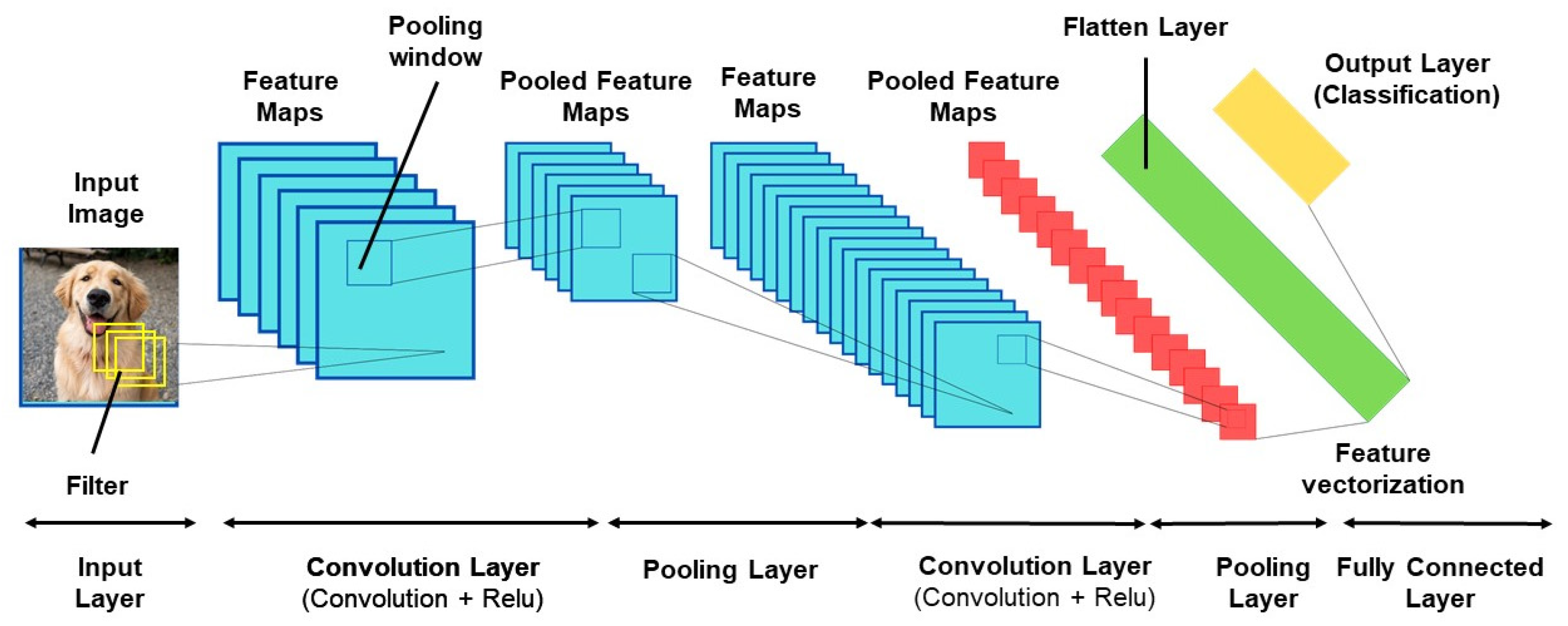
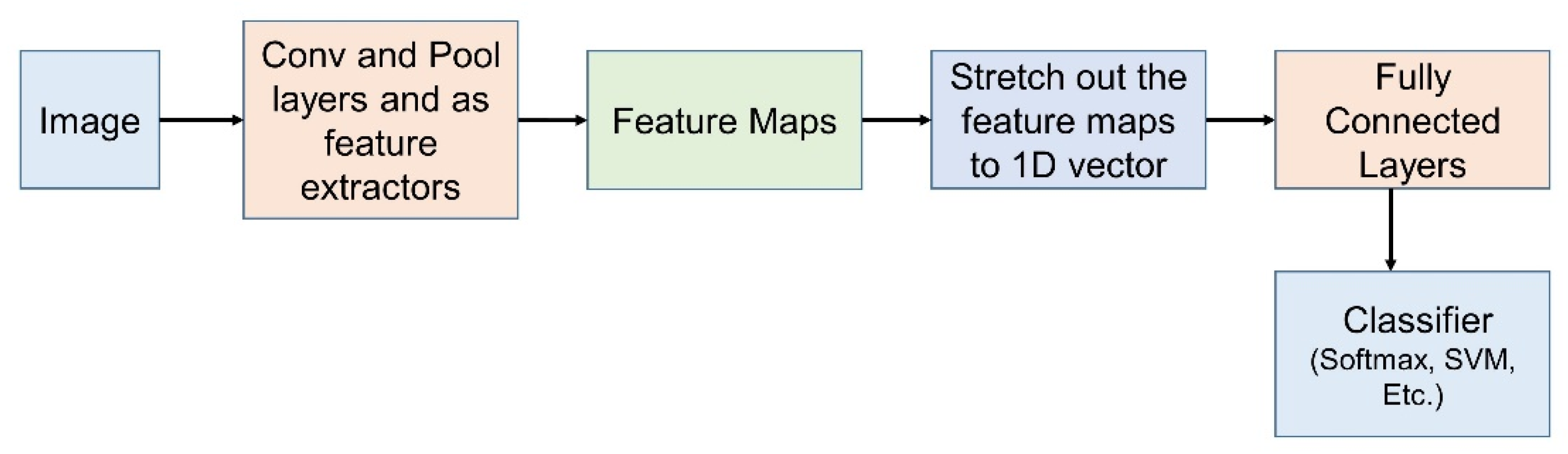
2.1. Building Blocks of CNN
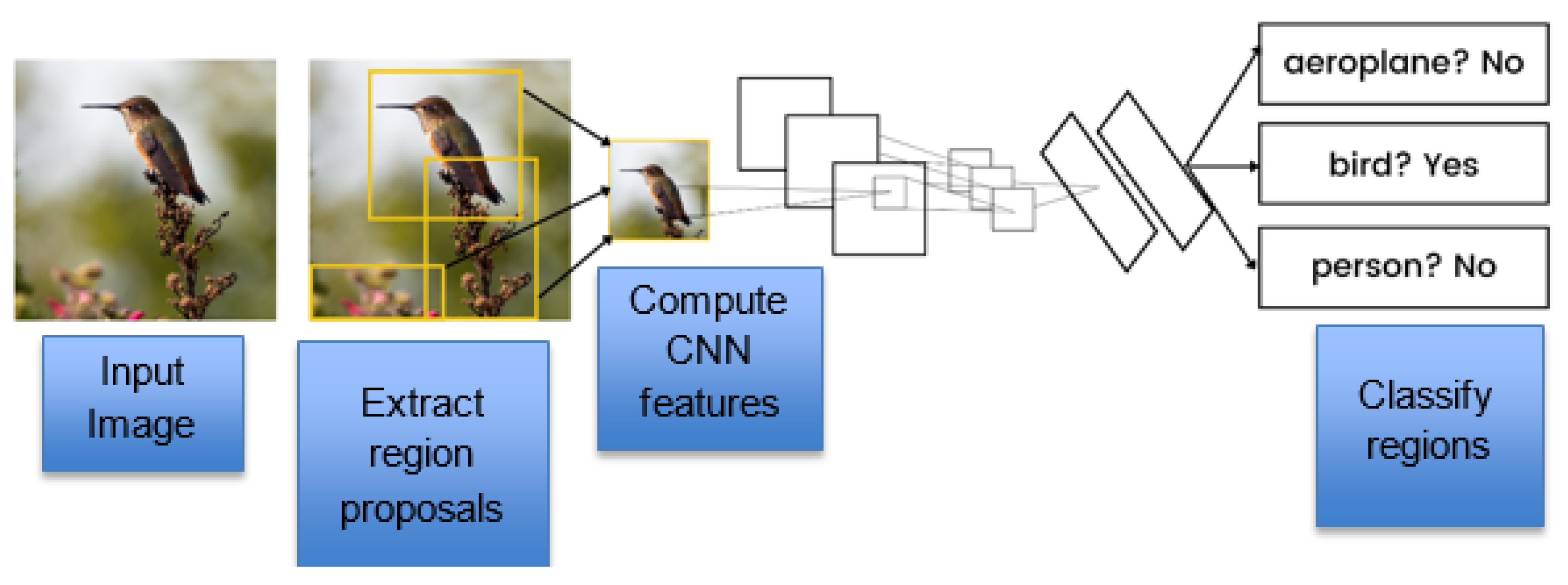
Figure 1 demonstrates the building block of CNN.
Convolution: The main step here constitutes feature extraction from the input image. It is the first step in CNN. There is an input image, a feature detector, and a feature map. The filter can be applied block by block to the input image.
ReLU: ReLU stands for a rectified linear unit and is the next step to the convolution layer. It is the activation function frequently used in CNN. Convolution is a linear operation, whereas the data of the real world is non-linear; however, other activation functions can also be applied like Sigmoid, Tanh and Leaky ReLU.
Pooling: The size of the representation of the input is reduced as the pooling progresses. With this, the detection of the objects becomes possible irrespective of their location. With the help of pooling, the number of required parameters is reduced, thereby reducing the computational power. Hence, it can control overfitting.
Flattening: one of the simple steps wherein the flattening is carried out of the pooled feature maps into a sequence of long vectors.
Fully connected layer: this helps to combine the attributes and features that can predict the classes.
The Figure 2 depicts the classification pipeline using CNN. The image is passed as an input to a stack of Conv and Pool layers which act as feature extractors. The feature maps are obtained as the output after the Conv and Pool layers are stretched out to a 1-dimensional vector. The 1-D vector is then passed on to the classification layer. The softmax translates the probability from the output score of the fully connected layer. Depending on the class having the highest probability, the name of the image is obtained.
The classification pipeline is modified to perform the localization using a CNN. For localization, the bounding box needs to be drawn around the object. In Figure 3, the classifier obtains the class scores and classifies the image using the softmax function. The BBox Regressor obtains the bounding box by using the L2 loss. The classifier and BBox Regressor are combined by considering the maximum confidence score and its corresponding coordinate to complete the localization.
There are various methods of object detection as described below:

2.1.1. R-CNN

R-CNN [8] in the Figure 4 comprises three parts: a region proposal, a feature extractor, and a classifier. A region proposal is a tool that generates and extracts region proposals. The feature extractor’s job is to extract the features out of each candidate region. The classifier then classifies the features as one of the known classes.
A bounding box region is proposed for the objects in the image with the help of a selective search. One of the simple examples of a CNN is object localization and recognition. Its disadvantage is that it is time-consuming because each of the candidate regions generated by the region proposal algorithm requires a CNN-based extraction pass.

2.1.2. Fast R-CNN

An R-CNN’s [9] drawback is that the training takes a long time and takes up much space. Hence, making predictions becomes very slow. In Fast R-CNN, the input is a set of region proposals. For feature extraction, a pre-trained CNN can be applied to it. The pooling layer, or the final layer, extracts features pertaining to a certain input candidate region. The two outputs—class prediction and the bounding box—are separated by the fully connected layer. The technique is then performed numerous times for each image.

2.1.3. Faster R-CNN

The architectural model was upgraded yet again for training and detecting speed. As part of the training, the region proposals were revised. The model’s test-time operation was improved to near real-time with a state-of-the-art performance due to these enhancements. There are two main modules of Faster R-CNN [10], namely the region proposal network and the Fast R-CNN. The RPN is used to propose the regions and the considerable objects in the region. Fast R-CNN extracts the features from the proposed regions and generates a class label and bounding box. Yi et al. presented a probabilistic faster R-CNN technique with a stochastic region to recognise and locate grasshoppers from a remote sensing image and achieved a 0.9263 f1-score [11].

2.1.4. Mask R-CNN

The Mask R-CNN [11] adapts a two-stage procedure, wherein the first stage is the RPN. In the next stage, in parallel to predicting the box offset and the class, Mask R-CNN also outputs a binary mask for each ROI. Mask R-CNN draws a dotted bounding box around each detected object. A class label is assigned to each detected object. The confidence score of the class label prediction is mentioned on the top-left corner of the bounding box. A polygon outline for the mask of each detected object is drawn, known as the object mask outline. The object mask indicates the fill of the polygon for the mask of each of the objects detected. The main limitation of this is that it falls short for real-time applications.

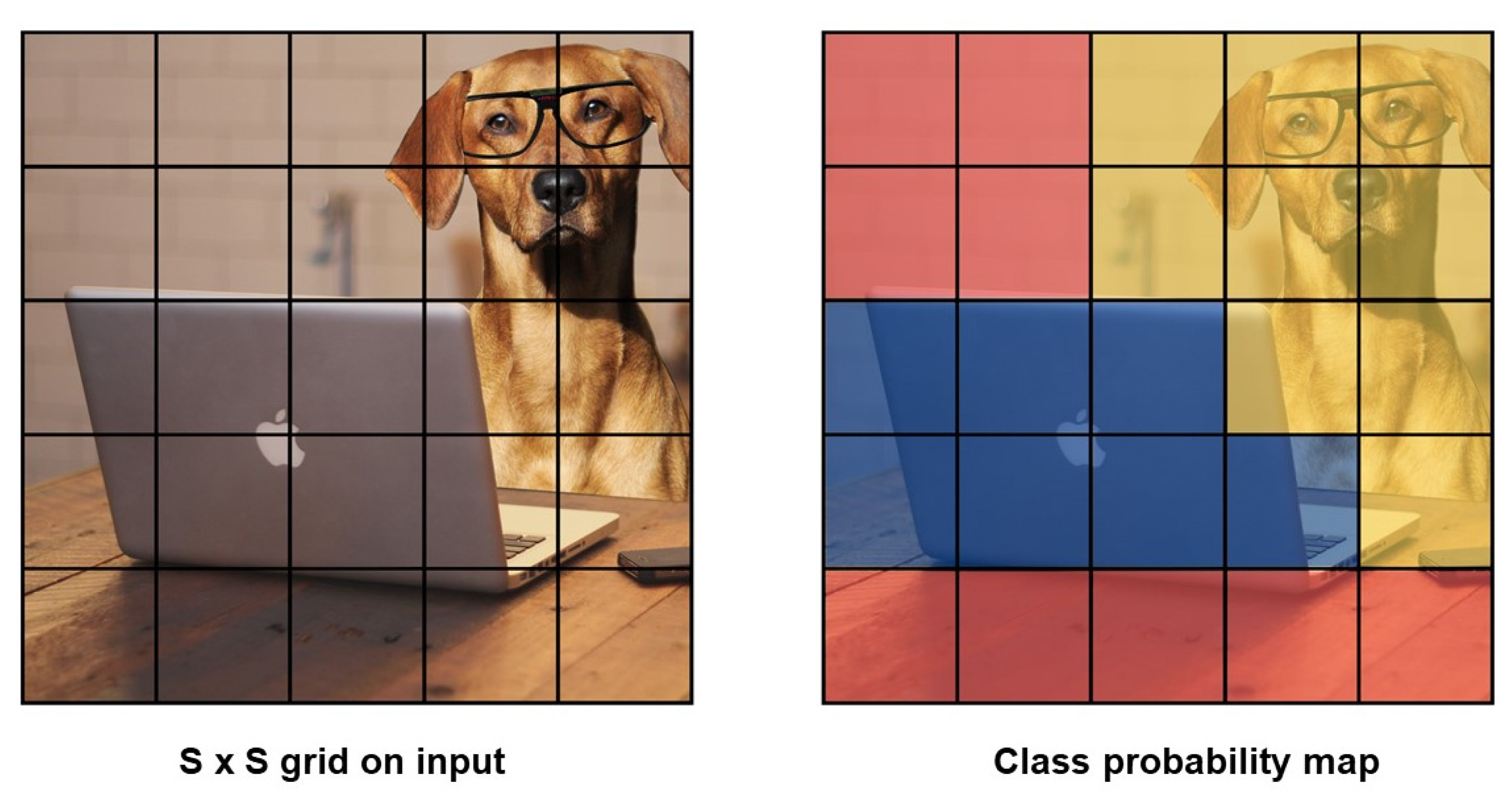
2.1.5. YOLO Versions

In YOLO (You Only Look Once) in the Figure 5, an image is fed to the single neural network and trained from scratch, thereby predicting the bounding box and class labels for each bounding box [12]. In this, the entire image is divided into grid cells, and each cell has the responsibility of predicting a bounding box only if the centre of the bounding box falls within it. The predicted bounding box involves x and y coordinates along with the width, height, and confidence. For each cell, a class prediction also plays a vital role.
For image classification, an image is fed as an input to the neural network, and a single class label along with the associated probability is obtained as the output. The class label characterizes the entire image. For object detection, either the (x, y) coordinate for each object or the list of the bounding boxes is required. Additionally, with each bounding box, the class label should also be associated.
The class label and the confidence score or the probability associated with each bounding box are obtained as the output. In this, the sliding window concept is utilized wherein the slide from either left to right or from right to left is performed to localize the objects at different locations. At varying scales, an image pyramid is used to detect the objects. Classification is carried out via a pre-trained CNN. At every stop, the region of interest is calculated and is fed as an input to the CNN to obtain the output classification for the region of interest. In the case where the probability of classification of the label is high compared to the threshold, the bounding box of the ROI is labelled as L. Continuing this process, we obtain the object detectors. Finally, NMS is applied to the bounding box in order to yield the final output. In general, this method is slow, while allowing a few errors in. This method can turn any random image classification network into an object detector. Thereby, it can avoid the need to train an object detector explicitly. Modwel et al. introduced a hybrid approach for real-time object detection. They combine three fundamental strategies to decrease frame scanning. The Recursive Density Estimation (RDE) technique selects the scan frames. The YOLO algorithm detects and recognises the objects in the selected frame with a 97% accuracy. The SURF algorithm tracks the detected items in consecutive frames [13].
The mean average precision (mAP) is used to assess the accuracy of the deep learning object detector. It is based on the intersection of all classes in our dataset (IoU) in the Figure 6.
Redmon et al. [14] introduced YOLO v2 and improvements were made in batch normalization, high resolution of the classifier, the use of anchor boxes, and the dimensionality clusters [15]. By adding the batch normalization to the architecture, the convergence of the model was increased, which led to faster training. The need for applying Dropout was eliminated. It was observed that there was an increase of 2% in the mAP from the basic YOLO. The input size in the previous YOLO was 224 × 244 during the training time, but during the time of detection, the image could be up to-the size 448 × 448. In YOLO v2, the fully connected layer was removed, and instead, the anchor boxes were added to predict the bounding box. With this, a decrease in the mAP was observed; however, the recall was found to increase.
YOLO v3 [16] utilizes the concept of multi-label classification. Salam et al. utilized YOLOv3 to detect things in interior environments like offices or rooms and to generate speech messages in Arabic sound for each object observed. The presented approach can detect six objects with a 99% accuracy [17]. Binary cross-entropy is used for every class label in YOLO v3, and a reduction in the computation complexity is seen by avoiding the softmax function. The cost function is also calculated differently in YOLO v3. If the anchor overlaps the ground truth, then the corresponding objectness should be 1. In earlier approaches, the ground truth object was only associated with one border-box. There was no classification if the bounding box was not assigned beforehand. YOLO v3 makes the detection at three different scales. Hong et al. presented an enhancement on the “you only look once” (YOLOv3) framework for ship detection in maritime surveillance using SAR and optical data. The improved YOLOv3 has the average accuracy of 93.56% and 95.52% on optical and SAR datasets, respectively [18]. The limitation as seen in YOLO v3 is that an increase in the grid size results in a greater number of anchor boxes which leads to an increase in the number of times for detection.
YOLO v4 is influenced by modern BoF (bag of freebies) and BoS (bag of specials) [19]. The BoF improve detector accuracy without increasing the inference time. The BoS, on the other hand, raise the inference cost but improve object detection accuracy. Jocher et al. proposed YOLOv5 [20]. Unlike previous releases, YOLO v5 is a PyTorch implementation rather than a Darknet derivative. One of the biggest enhancements is auto learning bounding box anchors.

2.1.6. RefineDet512

This is a single-shot based detector that has been found to achieve better accuracy than the two-stage methods. It consists of an anchor refinement module and an object detection module. The anchor refinement module filters out the negative anchors, which help to reduce the search space for the classifier by adjusting the size and location of the anchors for better initialization. The object detection module considers the refined anchors as input from the anchor refinement module to improve the multi-class label. Furlán et al. adapted the method of a single-shot-detector (SSD) network to detect rocks in planetary images [21]. The limitation observed in RefineDet 512 [20] is that as it is a two-step cascaded process, real-time detection is slow.

2.1.7. CenterNet

CenterNet [22] detects each object as a triplet, which improves both recall and precision. The CenterNet explores the centre part of the region, which is close to the geometric centre. If the predicted bounding box has a high IoU compared to the ground truth box, there is a high chance that the centre key point in its central region will be forecasted as the same class. The limitation seen in the CenterNet is that the addition of the extra branch to identify the centre key point potentially increases the overhead of object detection and reduces real-time performance.
The Table 1 summarizes the highlights and the limitations of the various methods of object detection.

3. Methods

In this section, the proposed architecture is explained in detail.

3.1. Proposed Architecture

In our proposed architecture, there are 22 convolution layers and 5 max-pooling layers. The first 16 convolution layers are used for extracting the features from the input image. The remaining 6 convolution layers are used for object detection which is depicted in Figure 7. It trains on a 608 × 608 image size. Mostly 3 × 3 and 1 × 1 filters are used, and they are double the number of filters after every pooling step. For end-to-end detection methods, the quality of the anchor box plays a vital role. The anchor boxes can be generated with a fixed size and scale; however, the generated anchor boxes by fixed size are usually suitable for the common sizes of objects, whereas the size of the objects may vary. After the analysis was carried out to detect the box of YOLOv2, it was observed that some unusual sizes of the objects were difficult to be detected and recognized. The unusual size of the object here, for example, was a size bigger than that of the truck. The sedan could be detected easily for the vehicle, but the difficulty was observed detecting the motorbike because of its size. Therefore, to improve the detection accuracy, it is better to generate an anchor box which matches most of the sizes of the ground truth. Consequently, in our work, a multi-scale anchor box was used. The grid size considered to detect the small objects was 19 × 19. In the last convolution layer, 675 output tensors were generated which was calculated based on the number of classes present in the dataset and the class presence probability with its bounding box coordinates. After generating the tensors, the anchor box was selected based on the information mentioned in Section 3.2. On each anchor box, regression was applied to predict the class of the object with its bounding box coordinates. Finally, a non-max suppression technique was applied with an IoU = 0.5 to select the bounding box having the highest probability among the overlapping bounding boxes.
In each grid cell, 9 anchor boxes with 3 different scales (1:1, 1:2, 2:1) were applied. Whether the object was of small size or with a large size, our method could recognize them well. Additionally, regardless of the variation of illumination intensity, our method could detect and recognize small objects, thereby demonstrating the strong robustness of our proposed method.

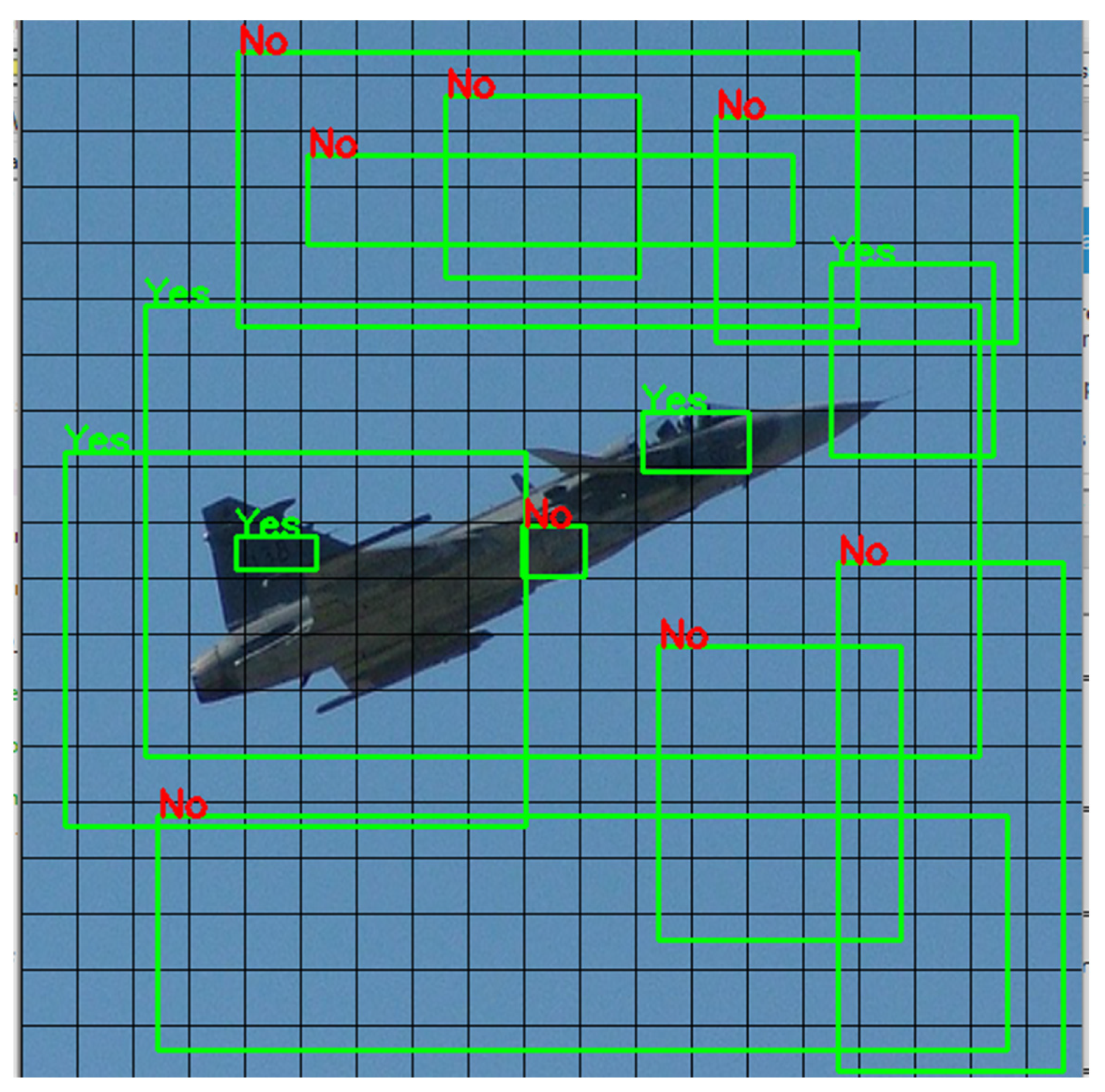
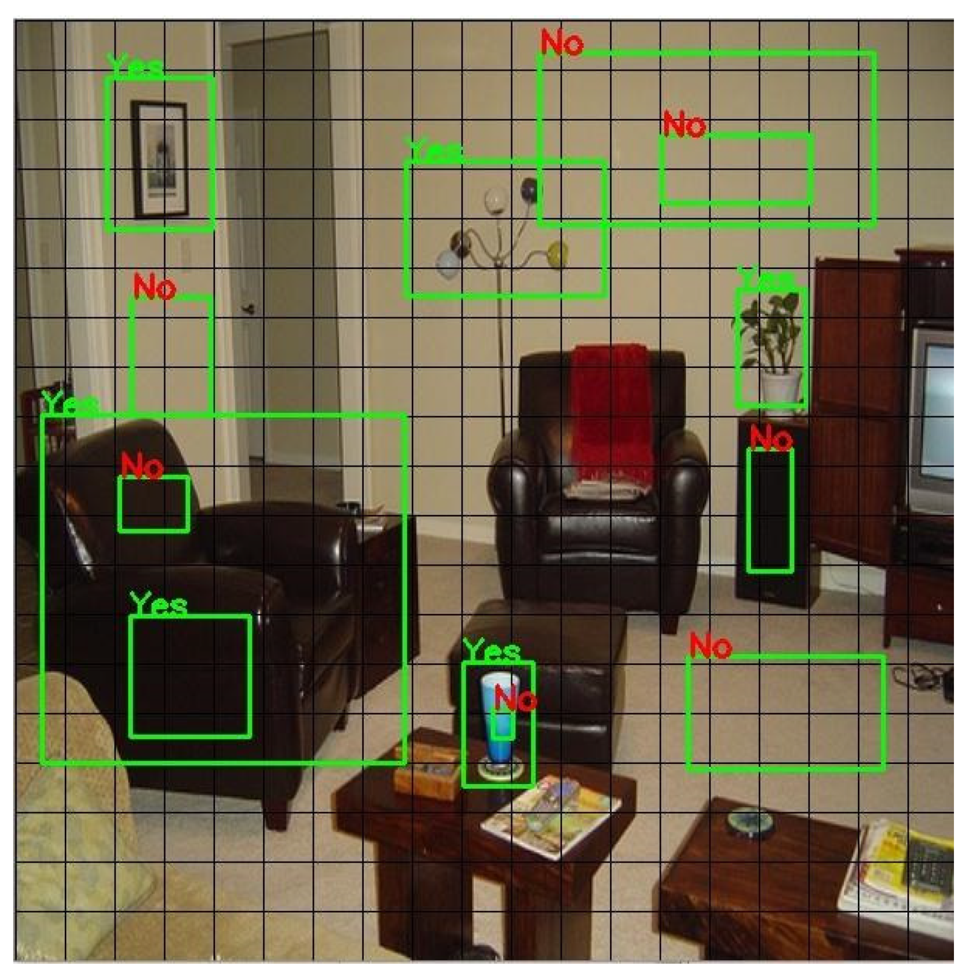
3.2. Efficient Multi-Scale Anchor Box Approach

Object detection models which use the anchor box approach generate feature maps to detect an object at the last convolution layer. These feature maps are used to predict the object from defined anchor boxes. It is not necessary that all the anchor boxes carry sufficient information to detect the object; however, the prediction score is calculated for every anchor box which leads to an increased execution (training and testing) time in object detection. Hence, real-time object detection becomes time-consuming and reduces the FPS rate. In our work, we introduced an efficient method to utilize the anchor box for prediction. The method was that a prediction was not applied for all anchor boxes as there was a chance that there would not be any information in a given anchor box, i.e., Figure 8 and Figure 9. In order to validate the information, anchor boxes were arranged in descending order by their sizes. If there was no information in a large size anchor box, there was no need to explore small size anchor boxes within the grid. This method was applied at the last layer convolution block which saved higher computation and memory costs. This method is explained in two parts.
(1)
An optimized multi-scale anchor box detects whether the information is present or not. This is done in the following manner:
  • Applying the canny edge detector algorithm [23] for only the anchor box portion. The canny edge detector algorithm requires a minimum and maximum threshold value to determine whether the obtained edge is weak or strong. To automate this process, the Otsu binary threshold [24] is used. This binary threshold gives the minValue and maxValue threshold.
  • The above step gives an output image wherein the frequency of black and white pixels is calculated. If the white pixels have a frequency of less than 30, then it indicates the absence of information. In all other cases, information is present. The threshold value of 30 is a hyper-parameter and is decided by the trial-and-error method. The value is considered for the Pascal VOC-2007 dataset.
(2)
To carry out the small object detection in an optimized way, the anchor boxes are arranged in descending order (i.e., large-scale anchor box first and then moving towards small sized anchor box). If the information is not present in the large-scale anchor box, there is no need to move to a small-scale anchor box. This saves execution time for each time predicting the prediction score of the information present in the given anchor box.
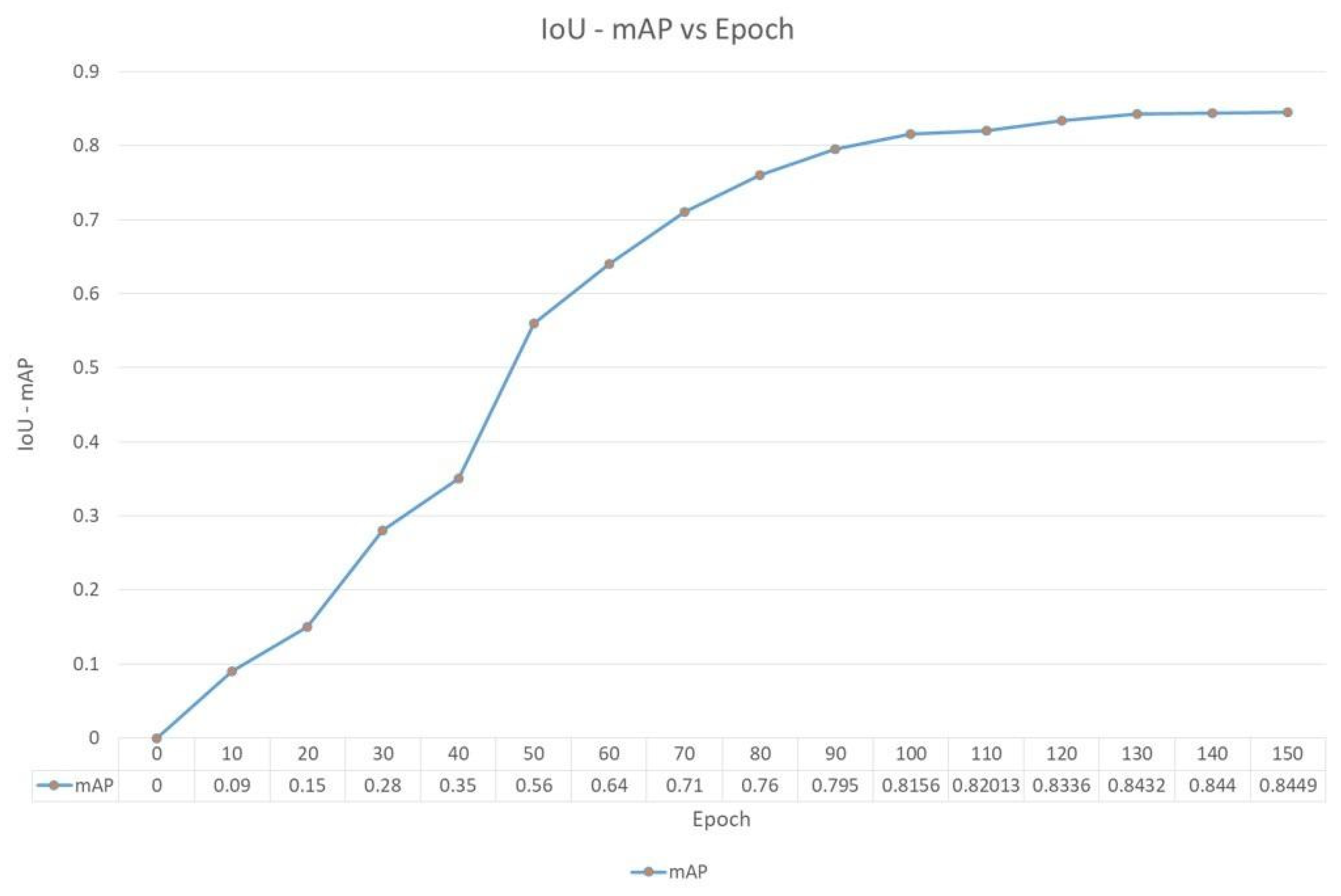
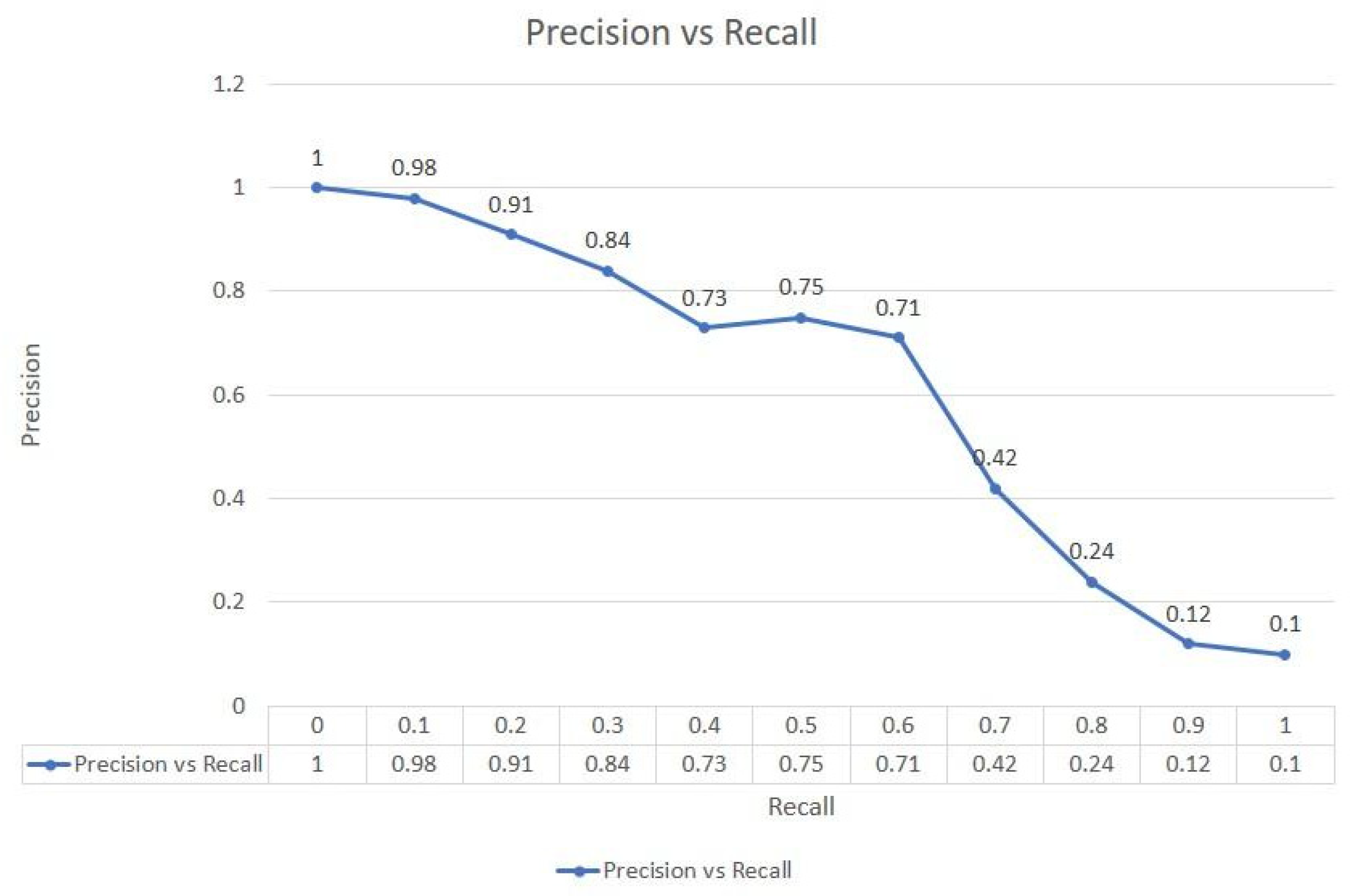
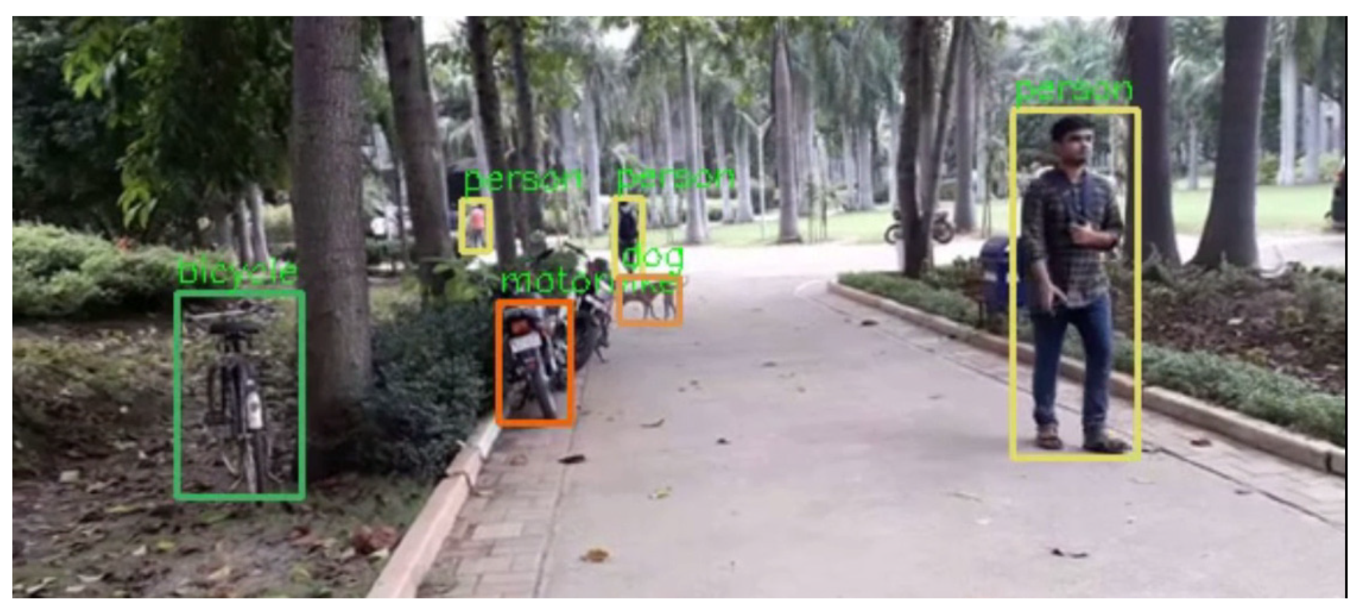
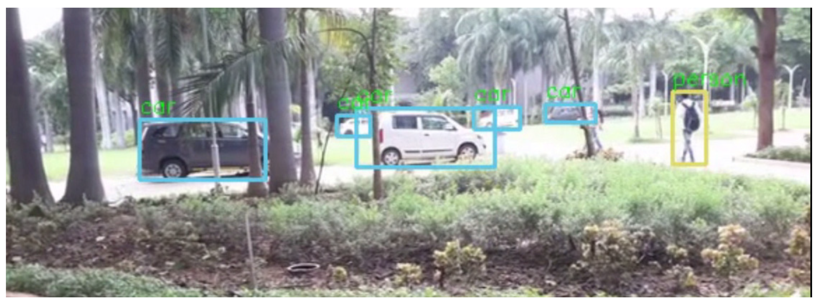
Figure 10 depicts the flowchart summarizing the training and the detection phase of the proposed model.

4. Experiments

This section describes the dataset used to perform the proposed work and compare the same with the existing work. The PASCAL VOC 2007 dataset was considered for the experiments [7]. This dataset consists of 20 classes (as mentioned below) for object recognition; it provides some sets of standardized image datasets. A common set of tools is provided to access the datasets as well as the annotations. This dataset was available from the VOC challenge links. There are mainly two competitions in it, namely, classification and detection. The detection seeks to forecast the bounding box and the class label from the target classes in the test image, while the classification aims to predict the absence/presence of the class example in the test image [7]. The Table 2 below compares the various object detection approaches implemented in the PASCAL VOC 2007 dataset and compares speed. It was observed that the mAP of the proposed model was far better as compared to the other object detection methods. The proposed model achieves a speed of 11 FPS over the baseline models on the Pascal VOC dataset.
In Table 3, the existing model is compared with the proposed model in terms of various parameters such as the grid size, several convolution layers, and the number of bounding boxes drawn per grid cell over the same baseline dataset, i.e., the Pascal VOC dataset. The existing YOLO model uses the 7 × 7 grid to divide the entire image, and the architecture of the YOLO model is such that it uses 24 convolutional layers. In YOLO, there was no concept of an anchor box used; however, in YOLO v2, the concept of an anchor box was introduced for object detection. Two bounding boxes per grid cell were used in YOLO, and the entire result was compared using the Pascal VOC dataset. The proposed model used the grid of 19 × 19 over the entire image. The number of convolutional layers was reduced from 24 to 22, and a multi-scale anchor box was introduced in our proposed model. Instead of using two bounding boxes per grid cell, the proposed model used nine bounding boxes per grid cell, with each bounding box having nine multi-scale anchors. The importance of using the multi-scale anchor box was to precisely detect the small objects and to detect and recognise the large-sized objects.
Table 4 shows that when the grid size was 19 × 19, the mAP obtained was 84.49, which is reasonably better than the other mAP of varying grid sizes. Table 5 considers the class-wise performance of the proposed model with the existing algorithms over the baseline Pascal VOC dataset. In the above-mentioned table, the average precision of every class present in the dataset is calculated and compared for the existing model with that of the proposed model. Lastly, the mAP is calculated wherein it can be seen that a fair amount of increase was observed in the proposed model.
Table 5 depicts the calculation of the learnable parameters and the FLOPS of our proposed model.
Table 6 shows the reason behind selecting the 19 × 19 grid size.
In our work, the value of dropout in the Figure 11 was considered wherein the loss value was minimal after successful completion of 150 epochs. In our work, the dropout value of 0.5 was considered when the loss obtained was 0.25, which is comparatively lower than the loss values of 2.4 and 1.5, respectively.
Figure 12 compares the epoch versus IoU accuracy. The X-axis is the number of epochs, and Y-axis indicates IoU accuracy. As the number of epochs starts increasing, it indicates that the model is being trained better and after 130 epochs, the value of the mAP starts stabilizing; hence, any value between 130–150 epochs can be considered to have a mAP of 84%. The number of epochs is considered as high as possible, and the training is terminated based on the error rates.
The learning rate is one of the important hyper-parameters which controls the change in the model with the estimated error whenever the weight is updated. The main challenge is choosing the learning rate, as too small a value may increase the training process and get stuck. In the below graph, for the learning rate of 0.0001, the loss was found to be minimum and the value was 0.25, therefore, in our work, a learning rate of 0.0001 was considered, as shown in Figure 13.
In Figure 14, the mAP was measured with the PASCAL VOC dataset. The chart shows the results for 256 × 256, 416 × 416 and 608 × 608 resolution of the images. It is seen that a higher resolution of the image shows a better mAP. The hardware configuration also plays a vital role to depict the computation process. As there was little change in the configuration, the mAP was not affected much. The changes in the FPS are also reported in the Figure 14. The higher resolution of the image improved the detection of the small objects significantly while also helping to detect the large objects. By reducing the resolution, the accuracy was also lowered by an average of 12%. The evaluation results depict that our scheme improved the performance of the computing.
Figure 15 depicts an inverse relationship between precision and recall, stating that the precision value lowers as the recall increases. In terms of object detection, as our model correctly recognised the objects, the chances of false recognition decreased. Figure 16 and Figure 17 illustrate the examples wherein the proposed model could identify the objects by their classes, and a class label was assigned on every detected object of varying size and shape from a video sequence.
Figure 18 illustrates at what size a small object could be detected. If the resolution of the image was 608 × 608 then the minimum object size of 40 × 47 could be detected and recognized accurately because the smallest size of an anchor box is considered 40 × 47.
The model failed to detect blurred objects. The objects Figure 19 which were not recognized by naked eyes, could not be detected by the proposed work.

5. Conclusions

In this work, a deep learning model based on the convolutional neural network is proposed, which is intended to accurately detect and recognize the varying size of objects from a video sequence. The paper starts with a detailed review of the deep learning algorithms and explains the architectures required for object detection and recognition. The existing models did not perform well for real-time object detection, specifically for small object detection. Therefore, to overcome this drawback, a model is proposed which can accurately detect and recognize the varying size of objects from a video sequence. A multi-scale anchor box is designed to capture the minor details of the object in the image. This improves the detection of state-of-the-art object detectors. The proposed model ensures the integrity of the feature of the large object and also preserves the full detail feature of the small objects by extracting the multi-scale feature of the image. The mean average precision of close to 84.49% and 11 FPS was achieved to detect the varying sizes of the objects for the network input size of 608 × 608. The proposed model also works well in detecting and recognizing objects in complex backgrounds. The number of parameters and FLOPS (the number of floating-point operations) of the proposed architecture are used to determine the complexity of the convolutional neural network and resulted in 31.57 M parameters and 22.95 FLOPS, respectively.
In future work, the proposed work can be examined on the MS-COCO dataset and can be optimized to run on edge devices in real time.

Author Contributions

Conceptualization, D.G. and K.K.; Methodology, D.G.; Validation, V.V., D.G. and K.K.; Formal Analysis, V.V.; Investigation, V.V. and K.K.; Resources, K.K.; Data Curation, D.G.; Writing—Original Draft Preparation, D.G. and K.K.; Writing—Review & Editing, V.V., D.G. and K.K.; Visualization, D.G. and K.K.; Supervision, V.V. and K.K.; Funding Acquisition, V.V. All authors have read and agreed to the published version of the manuscript.

Funding

This research received no external funding.

Institutional Review Board Statement

Not applicable.

Informed Consent Statement

Not applicable.

Data Availability Statement

Not applicable.

Conflicts of Interest

The authors declare no conflict of interest.

References

  1. Pouyanfar, S.; Sadiq, S.; Yan, Y.; Tian, H.; Tao, Y.; Reyes, M.P.; Shyu, M.L.; Chen, S.C.; Iyengar, S.S. A survey on deep learning: Algorithms, techniques, and applications. ACM Comput. Surv. (CSUR) 2018, 51, 1–36. [Google Scholar] [CrossRef]
  2. Guo, Y.; Liu, Y.; Oerlemans, A.; Lao, S.; Wu, S.; Lew, M.S. Deep learning for visual understanding: A review. Neurocomputing 2016, 187, 27–48. [Google Scholar] [CrossRef]
  3. Silver, D.; Huang, A.; Maddison, C.J.; Guez, A.; Sifre, L.; van den Driessche, G.; Schrittwieser, J.; Antonoglou, I.; Panneershelvam, V.; Lanctot, M.; et al. Mastering the game of Go with deep neural networks and tree search. Nature 2016, 529, 484–489. [Google Scholar] [CrossRef] [PubMed]
  4. Palmer, R.; West, G.; Tan, T. Scale Proportionate Histograms of Oriented Gradients for Object Detection in Co-Registered Visual and Range Data. In Proceedings of the 2012 IEEE International Conference on Digital Image Computing Techniques and Applications (DICTA), Fremantle, Australia, 3–5 December 2012; pp. 1–8. [Google Scholar]
  5. Lowe, D.G. Distinctive Image Features from Scale-Invariant Keypoints. Int. J. Comput. Vis. 2004, 60, 91–110. [Google Scholar] [CrossRef]
  6. Leonardis, A.; Bischof, H.; Pinz, A. SURF: Speeded Up Robust Features. In Computer Vision–ECCV 2006, Proceedings of the 9th European Conference on Computer Vision, Graz, Austria, 7–13 May 2006; Springer: Berlin/Heidelberg, Germany, 2006; Part I; Volume 3951, pp. 407–417. [Google Scholar]
  7. Everingham, M.; Van Gool, L.; Williams, C.K.I.; Winn, J.; Zisserman, A. The Pascal Visual Object Classes (VOC) Challenge. Int. J. Comput. Vis. 2010, 88, 303–338. [Google Scholar] [CrossRef] [Green Version]
  8. Girshick, R.; Donahue, J.; Darrell, T.; Malik, J. Rich feature hierarchies for accurate object detection and semantic segmentation. In Proceedings of the IEEE Conference on Computer Vision and Pattern Recognition, Columbus, OH, USA, 23–28 June 2014; pp. 580–587. [Google Scholar]
  9. Girshick, R. Fast R-CNN. In Proceedings of the 2015 IEEE International Conference on Computer Vision (ICCV), Santiago, Chile, 7–13 December 2015; pp. 1440–1448. [Google Scholar]
  10. Ren, S.; He, K.; Girshick, R.; Sun, J. Faster R-CNN: Towards real-time object detection with region proposal networks. IEEE Trans. Pattern Anal. Mach. Intell. 2017, 39, 1137–1149. [Google Scholar] [CrossRef] [PubMed] [Green Version]
  11. Yi, D.; Su, J.; Chen, W.-H. Probabilistic faster R-CNN with stochastic region proposing: Towards object detection and recognition in remote sensing imagery. Neurocomputing 2021, 459, 290–301. [Google Scholar] [CrossRef]
  12. He, K.; Gkioxari, G.; Dollár, P.; Girshick, R. Mask r-cnn. In Proceedings of the IEEE International Conference on Computer Vision, Venice, Italy, 29 October 2017; pp. 2961–2969. [Google Scholar]
  13. Modwel, G.; Mehra, A.; Rakesh, N.; Mishra, K.K. A Robust Real Time Object Detection and Recognition Algorithm for Multiple Objects. Recent Adv. Comput. Sci. Commun. 2021, 14, 331–338. [Google Scholar] [CrossRef]
  14. IoU Accuracy. Available online: https://www.pyimagesearch.com/2016/11/07/intersection-over-union-ioufor-object-detection/ (accessed on 25 July 2021).
  15. Redmon, J.; Farhadi, A. YOLO9000: Better, Faster, Stronger. In Proceedings of the IEEE Conference on Computer Vision and Pattern Recognition, Honolulu, HI, USA, 21–26 July 2017; pp. 6517–6525. [Google Scholar] [CrossRef] [Green Version]
  16. Redmon, J.; Farhadi, A. Yolov3: An incremental improvement. arXiv 2018, arXiv:1804.02767. [Google Scholar]
  17. Salam, H.; Jaleel, H.; Hameedi, S. You Only Look Once (YOLOv3): Object Detection and Recognition for Indoor Environment. Multicult. Educ. 2021, 7, 171. [Google Scholar]
  18. Hong, Z.; Yang, T.; Tong, X.; Zhang, Y.; Jiang, S.; Zhou, R.; Han, Y.; Wang, J.; Yang, S.; Liu, S. Multi-Scale Ship Detection From SAR and Optical Imagery Via A More Accurate YOLOv3. IEEE J. Sel. Top. Appl. Earth Obs. Remote Sens. 2021, 14, 6083–6101. [Google Scholar] [CrossRef]
  19. Bochkovskiy, A.; Wang, C.Y.; Liao, H.Y.M. YOLOv4 Optimal Speed and Accuracy of Object Detection. In Proceedings of the Computer Vision and Pattern Recognition. arXiv 2020, arXiv:2004.10934. [Google Scholar]
  20. PyTorch Hub. Ultralytics/yolov5: v4.0—nn.SiLU() Activations, Weights & Biases Logging, PyTorch Hub Integration. 2021. Available online: https://codechina.csdn.net/ForrestGump92/yolov5/-/tree/silu (accessed on 26 November 2021).
  21. Han, G.; Zhang, X.; Li, C. Single shot object detection with top-down refinement. In Proceedings of the 2017 IEEE International Conference on Image Processing (ICIP), Beijing, China, 17–20 September 2017; pp. 3360–3364. [Google Scholar]
  22. Furlán, F.; Rubio, E.; Sossa, H.; Ponce, V. CNN based detectors on planetary environments: A performance evaluation. Front. Neurorobot. 2020, 14, 85. [Google Scholar] [CrossRef] [PubMed]
  23. Duan, K.; Bai, S.; Xie, L.; Qi, H.; Huang, Q.; Tian, Q. CenterNet: Keypoint Triplets for Object Detection. In Proceedings of the 2019 IEEE/CVF International Conference on Computer Vision (ICCV), Seoul, Korea, 27–28 October 2019; pp. 6568–6577. [Google Scholar]
  24. Canny Edge Detector Algorithm. Available online: https://towardsdatascience.com/canny-edge-detectionstep-by-step-in-python-computer-vision-b49c3a2d8123 (accessed on 12 August 2021).
Figure 1. Building blocks of CNN.
Futureinternet 13 00307 g001
Figure 2. Classification pipeline using CNN.
Futureinternet 13 00307 g002
Figure 3. Detection pipeline using CNN.
Futureinternet 13 00307 g003
Figure 4. Architecture of R-CNN.
Futureinternet 13 00307 g004
Figure 5. S × S grid distribution and class distribution map of YOLO.
Futureinternet 13 00307 g005
Figure 6. IOU calculation [14].
Futureinternet 13 00307 g006
Figure 7. Architecture of proposed model.
Futureinternet 13 00307 g007
Figure 8. Efficient multi-scale anchor box (Example 1).
Futureinternet 13 00307 g008
Figure 9. Efficient multi-scale anchor box (Example 2).
Futureinternet 13 00307 g009
Figure 10. Flowchart of the training and detection phase of the proposed model.
Futureinternet 13 00307 g010
Figure 11. Comparison of Loss vs. Epoch @ Dropout.
Futureinternet 13 00307 g011
Figure 12. Comparison of IoU mAP vs. Epoch.
Futureinternet 13 00307 g012
Figure 13. Comparison of Loss vs Epoch @ Learning Rate.
Futureinternet 13 00307 g013
Figure 14. Comparison of FPS and mAP on various resolutions using different configurations of CPU and GPU.
Futureinternet 13 00307 g014
Figure 15. Comparison between Precision vs. Recall.
Futureinternet 13 00307 g015
Figure 16. Object detection and recognition from a video sequence (Example 1).
Futureinternet 13 00307 g016
Figure 17. Object detection and recognition from a video sequence (Example 2).
Futureinternet 13 00307 g017
Figure 18. Minimum size of object detection.
Futureinternet 13 00307 g018
Figure 19. Object detection and recognition from an image (Example 3).
Futureinternet 13 00307 g019
Table 1. Comparison of methods of object detection.
ModelHighlightsLimitations
R-CNNIntroduced for obtaining better accuracy as compared to HOG. Uses selective search because CNN cannot run on too many patches created by the sliding window detector. The first model for integrating the RP methods with the CNN; improvement in the performance observed with respect to the previous state-of-the-art methods.Training is expensive in time and space. Testing is slow.
Fast R-CNNend-to-end detector training; design of a layer of RoI pooling; the multi-task objective of having both classification head and bounding box regression head reduces the overall training time and increases the accuracy.Takes more execution time for real-time applications.
Faster R-CNNInstead of a selective search approach, an RPN is proposed for the generation of high-quality region proposals. Introduces invariant translation and multi-scale anchor boxes as references in RPN. Comparatively faster in magnitude than Fast R-CNN without the loss in performance.Complex training and falls short of real-time.
Mask R-CNNExtends Faster R-CNN by adding a branch to predict the object mask along with the existing branch for bounding box prediction; outstanding performance.Falls short of real-time application.
YOLO (You Only Look Once)The classification score for each box is predicted for every class in training. Image is divided into grids having the coordinates—SXS, and hence total boxes predicted are SXSXN. It sees the complete image at once.Struggles for a small object.
YOLO v1A first efficient unified detector, significantly faster than other previous detectors.A decrease in accuracy as compared to the state-of-the-art detectors and struggles for small object detection.
YOLO v2Uses the number of existing strategies to improve the accuracy and speed.Not good in detecting small objects.
YOLO v3At three different scales, detection is carried out by applying the 1 × 1 detection kernel to feature maps of three different sizes at three separate locations in the network.An increase in the grid size results in an increased number of anchor boxes which leads to an increase in the number of times for detection.
RefineDet 512Refines the sizes and the location of the anchor box with the help of the anchor refinement module and object detection module.As it is a two-step cascaded process, real-time detection is slow.
CenterNetDetects each of the objects as triplets, which improves both the recall and the precision. It explores the central part of the proposal, which is the region close to the geometric centresAdded an extra branch to identify the centre key point, which potentially increases object detection overhead and reduces real-time performance.
Table 2. Comparison of existing models with a proposed model in terms of mAP and speed.
Sr. No.ModelYearmAP (%)Speed (FPS *)
1R-CNN201466.00.05 FPS
2Fast R-CNN201570.00.5 FPS
3Faster R-CNN201573.27 FPS
4Mask R-CNN201778.20.1 FPS
5YOLO v1201663.414 FPS
6YOLO v2201776.0112 FPS
7YOLO v3201881.79 FPS
8YOLO v4202083.510 FPS
9YOLO v5202184.126 FPS
10RefineDet512201881.86 FPS
11CenterNet201978.70.3 FPS
12CenterNet2202181.692 FPS
13Proposed Model202184.4911 FPS
* indicates that the result of FPS is calculated by running the algorithms on 4 GB GPU, NVIDIA GTX 1050 Ti.
Table 3. Comparison of the existing model with the proposed model on various parameters.
CharacteristicsExisting ModelProposed Model
Grid7 × 7 grid19 × 19 grid
Layers24 convolutional layers23 convolutional layers
Anchor BoxesFixed-size anchor boxesMulti-scale anchor box
Bounding box/cell2 bounding box/cell9 bounding boxes/cells, with each bounding box having 9 multi-scale anchors.
DatasetPASCAL VOC 2007 dataset with 20 classes
and 9963 images containing 24,640 annotated objects.
Table 4. Comparison of mAP on various grid sizes.
ModelsGrid SizemAP (%)
YOLO7 × 763.4
9 × 968.93
11 × 1177.39
Proposed Model15 × 1580.29
19 × 1984.49
Table 5. Calculation of learnable parameters and FLOPS for the proposed model.
Layer No.Layer TypeFiltersKernel SizeOutput#Parameters#FLOPS
1Convolutional323 × 3608 × 608 × 32864319,389,696
2Max-2 × 2304 × 304 × 32011,829,248
3Convolutional643 × 3304 × 304 × 6418,4321,703,411,712
4Max-2 × 2152 × 152 × 6405,914,624
5Convolutional1283 × 3152 × 152 × 12873,7281,703,411,712
6Convolutional641 × 1152 × 152 × 648192189,267,968
7Convolutional1283 × 3152 × 152 × 12873,7281,703,411,712
8Max-2 × 276 × 76 × 12802,957,312
9Convolutional2563 × 376 × 76 × 256294,9121,703,411,712
10Convolutional1281 × 176 × 76 × 12832,768189,267,968
11Convolutional2563 × 376 × 76 × 256294,9121,703,411,712
12Convolutional1281 × 176 × 76 × 12832,768189,267,968
13Convolutional2563 × 376 × 76 × 256294,9121,703,411,712
14Max-2 × 238 × 38 × 25601,478,656
15Convolutional5123 × 338 × 38 × 5121,179,6481,703,411,712
16Convolutional2561 × 138 × 38 × 256131,072189,267,968
17Convolutional5123 × 338 × 38 × 5121,179,6481,703,411,712
18Convolutional2561 × 138 × 38 × 256131,072189,267,968
19Convolutional5123 × 338 × 38 × 5121,179,6481,703,411,712
20Convolutional2561 × 138 × 38 × 256131,072189,267,968
21Max-2 × 219 × 19 × 2560739,328
22Convolutional5123 × 319 × 19 × 512235,9296851,705,856
23Convolutional10241 × 119 × 19 × 1024524,288189,267,968
24Convolutional5123 × 319 × 19 × 5124,718,5921,703,411,712
25Convolutional10241 × 119 × 19 × 1024524,288189,267,968
26Convolutional5123 × 319 × 19 × 5124,718,5921,703,411,712
27Convolutional10243 × 319 × 19 × 10244,718,5921,703,411,712
28Convolutional6751 × 119 × 19 × 675691,200249,523,200
23,312,224
=23.31 M
23,398,622,208
=23.39 BFLOPS
Table 6. Class-wise performance of the existing models with the proposed model using PASCAL VOC 2007 dataset.
Class\ModelR-CNNFast R-CNNFaster R-CNNMask R-CNNYOLO v1YOLO v2YOLO v3YOLO v4YOLO v5RefineDetCenterNetCenterNet2Proposed Model
Aeroplane77.284.284.188.97786.387.290.190.588.786.189.689.7
Bike76.478.981.28667.284.388.387.689.68787.290.891.4
Bird68.875.275.480.269.274.878.979.578.583.282.485.489.1
Boat50.353.656.361.143.459.265.470.275.476.567.173.269.4
Bottle36.749.262.767.542.368.172.574.577.36860.156.475.2
Bus75.877.579.484.268.379.883.286.384.588.583.187.584.4
Car69.673.277.28268.576.583.488.192.488.782.785.491.3
Cat87.385.884.989.781.490.694.295.398.589.287.788.592.7
Chair42.245.657.161.953.764.268.370.871.266.561.764.268.4
Cow70.277.178.683.460.878.281.283.481.287.982.489.483.8
Table52.253.162.270.158.263.771.372.375.47568.478.374.9
Dog85.586.185.390.177.289.394.496.59786.889.489.993.1
Horse78.580.482.186.972.382.687.683.582.489.284.988.589.4
Motorbike78.878.983.688.471.383.488.189.591.587.886.389.491.2
Person68.379.378.983.763.581.593.395.695.984.785.786.594.8
Plant33.140.144.24948.952.871.375.476.556.262.360.574.1
Sheep66.372.673.478.259.477.678.376.474.383.284.385.679.3
Sofa63.768.462.367.154.869.875.279.580.378.773.178.478.7
Train76.280.381.287.273.985.185.485.984.788.185.485.889.4
TV62.960.573.878.656.772.486.589.685.382.373.980.589.5
mAP667073.278.263.476.881.783.584.1281.878.781.6984.49
Publisher’s Note: MDPI stays neutral with regard to jurisdictional claims in published maps and institutional affiliations.

