Abstract
A heterogeneous system can be portrayed as a variety of unlike resources that can be locally or geologically spread, which is exploited to implement data-intensive and computationally intensive applications. The competence of implementing the scientific workflow applications on heterogeneous systems is determined by the approaches utilized to allocate the tasks to the proper resources. Cost and time necessity are evolving as different vital concerns of cloud computing environments such as data centers. In the area of scientific workflows, the difficulties of increased cost and time are highly challenging, as they elicit rigorous computational tasks over the communication network. For example, it was discovered that the time to execute a task in an unsuited resource consumes more cost and time in the cloud data centers. In this paper, a new cost- and time-efficient planning algorithm for scientific workflow scheduling has been proposed for heterogeneous systems in the cloud based upon the Predict Optimistic Time and Cost (POTC). The proposed algorithm computes the rank based not only on the completion time of the current task but also on the successor node in the critical path. Under a tight deadline, the running time of the workflow and the transfer cost are reduced by using this technique. The proposed approach is evaluated using true cases of data-exhaustive workflows compared with other algorithms from written works. The test result shows that our proposed method can remarkably decrease the cost and time of the experimented workflows while ensuring a better mapping of the task to the resource. In terms of makespan, speedup, and efficiency, the proposed algorithm surpasses the current existing algorithms—such as Endpoint communication contention-aware List Scheduling Heuristic (ELSH)), Predict Earliest Finish Time (PEFT), Budget-and Deadline-constrained heuristic-based upon HEFT (BDHEFT), Minimal Optimistic Processing Time (MOPT) and Predict Earlier Finish Time (PEFT)—while holding the same time complexity.
1. Introduction
The emerging field of cloud computing is spreading computations that bring versatile scalable services on necessity over the Internet by the virtualization of hardware and software. The cloud comprises a heterogeneous system which can be well-portrayed as a multiple unlikely set of resources, such as virtual machines or links, which can be locally or hugely spread, that are exploited to produce data-intensive and computationally intensive applications. A highly capable task-scheduling algorithm is very important for attaining a better performance in cloud computing. The overall task scheduling is to give the task of an application to suitable processors and then hand over the objective to execute on an appropriate resource [1,2]. The static model is such that, when the characteristics of the tasks are known in advance, the proficiency in executing the scientific workflow applications on diverse systems is based on the methods used to distribute the tasks to an appropriate resource. The core benefits of clouds are their availability, reliability, scalability, and flexibility where the cloud provider has the ability to lease and release resources/services as per the user’s requirements. The cloud providers Amazon EC2, Digital Ocean, Microsoft Azure, Rackspace Open Cloud, Google Compute Engine, IBM Smart Cloud Enterprise, Cloud Stack, Open Nebula, and Go Grid offer resources/services [3].
Scientific workflows are depicted by a directed acyclic graph (DAG) in which nodes signify tasks in the application and the edges signify dependencies between the tasks. Each node label represents the time of the execution of the task, and the edges represent the transfer costs among the tasks. The scientific workflows are specifically associated with scientific denominations like bioinformatics and biodiversity. BioBIKE and astronomy present a robust circumstance for the utilization of cloud implementation. Workflow planning is a series consisting of allocating the dependent tasks on the appropriate resources in such a way that the complete workflow will be able to finish its implementation inside the user’s mentioned quality of service (QoS) constraints. The processing of workflows involves enormous computation and communication costs. The aim is to allocate the objectives onto appropriate virtual machines and sort the sequence of implementations so that the task priority needs are satisfied and a minimum implementation time and reduced cost are obtained. Moreover, realistic scheduling approaches must use only a few resources and must have less time complexity. The task-scheduling problem is known to be NP-complete, and the challenges in the field are mainly focused on getting low-complexity heuristics that yield excellent schedules.
Scheduling algorithms are usually grouped into two types, namely heuristic and meta-heuristic. For a broad range of given problems, heuristic is defined as an approximate solution and problem-dependent and metaheuristics is defined as problem-independent where a solution can be received for which it can be proved its closeness to the optimal solution. The heuristic algorithms that are frequently operated in a heterogeneous environment have varied and versatile virtual machines, such as cloud data centers, etc. They consist of duplication-based, list-based, and clustering-based algorithms. Some of the meta-heuristic algorithm examples are as follows—genetic algorithm (GA), firefly optimization (FO), artificial neural network (ANN), cat swarm optimization (CSO), particle swarm optimization (PSO), simulated annealing (SA), tabu search (TS), and ant colony optimization (ACO) can provide an optimal solution. On relating the heuristic technique with the metaheuristic technique, when the count of tasks is multiplied, the makespan of the metaheuristic techniques proliferates continuously.
The heuristic algorithm can be separated into a duplication-based scheduling algorithm [4], a list-scheduling algorithm, and a clustering scheduling algorithm. There are two important stages in the list-scheduling algorithm. In the first stage, the priority is set to the tasks by computing the rank to every task in the DAG. In the next stage, the corresponding virtual machine is chosen to complete the task.
The methodology behind the clustering-based scheduling technique is to find the tasks in the DAG which would be executed on the self-same virtual machine (VM). There are two phases in the clustering-based technique. Phase 1 is the clustering phase, where the tasks are segregated into a collection of disjoint clusters. Phase 2 is the merging phase, where the clusters are merged so that they can be assigned or allocated to the confined measure of processors at runtime. One of the best widespread heuristic clustering-based algorithms is the dominant sequence clustering (DSC) [5].
The technique that replicates the parent tasks by using the time in which the processors are idle is termed a duplication-based scheduling algorithm [6]. This collection of algorithms performs task scheduling by the allocation of its redundant tasks. Hence, this technique can decrease the inter-related communication overhead. Conversely, these techniques are impractical due to their increased time complexity.
The genetic algorithm (GA) which is a meta-heuristic algorithm, is renowned and extensively discussed. In this type, there are three stages, which are called the selection, the crossover, and the mutation stage. In the first one (selection stage), initially, the population set is generated and the parents are selected from ‘individuals’ of the group. In the crossover stage, the parents hybridize to yield children that are ‘offspring’, and in the mutation stage, the children could be changed as per the mutation rules.
The scheduling algorithms aim to reduce the total execution time without making a note of the resource access cost. However, resources of different competencies at different costs are provided by the service provider in the cloud environment. More rapid resources are always more expensive than the slow one. Therefore, various planning techniques of the same workflow using dissimilar hardware/resources may result in a dissimilar schedule length ratio and a dissimilar price. Therefore, the workflow planning issue in cloud computing entails both cost and time limitations which need to be fulfilled as per the user’s requirement. The budget constraint confirms that the cost mentioned by the user has not been exceeded, and the deadline constraint confirms that the workflow is implemented within the specified time limit. Decent heuristic attempts have been made to handle both these constraints equally and achieve a better result.
The two objectives in workflows are minimizing the makespan and minimizing the implementation costs. In this paper, a new Predict Optimistic Time and Cost (POTC) is recommended to plan workflow applications to cloud computing services that reduce the implementation cost (i.e., the sum of transfer cost and VM price) and the total execution time (i.e., the addition of data transmission time and execution time) for executing the scientific workflows simultaneously. In this paper, the major parameter that has an influence on the cost in the heterogeneous system is considered. A system with a group of virtual machines and various communication links is exhibited as a heterogeneous system. In the cloud heterogeneous system, every single processor can transfer information with numerous other processors concurrently [7]. The mapping of tasks to the resource consists of two phases. In the initial phase, the tasks are ordered based on the rank and in phase two the planner maps the tasks on to the resource with respect to resource cost, transfer cost, implementation time, and earlier finish time from the pool of resources in a way that the total implementation time and overall cost of executing the entire workflow are reduced simultaneously based upon the auxiliary deadline and auxiliary budget of every workflow task. The planned heuristic, explicitly POTC, depends upon the PEFT algorithm, which reduces the overall workflow implementation time without bearing in mind the budget and cost restraints while making the planning decisions. The projected heuristic algorithm grants a valuable trade-off between cost and makespan under said constraints.
This finding is ordered as follows: the background of the task scheduling problem is presented in this section. In the second section, we the review of existing scheduling algorithms on the heterogeneous environment is extended. In Section 3 the application and the scheduling models are explained. In Section 4, we project the proposed POTC algorithm is projected and the contrast with the existing scheduling heuristic is explained. In Section 5 the results and comparison with the existing models are discussed, and, finally, Section 6 contains an elaborate conclusion.
2. Literature Survey
In this section, a review of task scheduling algorithms in scientific workflows has been studied mostly on list-based heuristics. For the past few years, research has focused on the workflow scheduling algorithm, in order to discover suboptimal results in a reasonably short duration. High-quality schedules are normally generated at a sensible cost using list-based scheduling heuristics. List-based scheduling heuristics have a lower complexity of time, and their results signify a lesser processor load when compared to other scheduling strategies, like clustering algorithms and task duplication strategies [8,9,10]. Many heuristic algorithms like Heterogeneous Earlier Finish Time (HEFT), Dynamic Scheduling-of-Bag-of-Tasks-based workflows (DSB), Budget-and Deadline-constrained heuristic-based upon HEFT (BDHEFT), Critical Path on Processor (CPOP), and Predict Earliest Finish Time (PEFT). Out of these, PEFT outperforms in terms of implementation time. However, all these heuristics try to diminish the implementation time without bearing in mind the cost of executing the workflow tasks.
Topcuoglu [11] has proposed a list-based scheduling algorithm with the aim of increasing the performance and fast scheduling time. The HEFT algorithm calculates the upward rank for all the tasks in the level and sort in descending order of rank. The task with the highest upward rank is selected first and assigns the same to the processor which reduces its earliest finish time and minimizes the makespan under no restraints. However, their solution does not meet the deadline constraint, and the communication cost is not considered. The HEFT algorithm is tested for heterogeneous systems.
Verma [12] presented a Budget-and Deadline-constrained Heterogeneous Earliest Finish Time (BDHEFT) with the aim of reducing the time and cost below the deadline and budget constraint. BDHEFT is an extension of HEFT with heterogeneous resources over the cloud. The algorithm outperforms in terms of monetary cost and makespan. However, they have not taken the transfer cost and communication time into consideration.
Hamid [13] has proposed an algorithm for heterogeneous computing systems named Predict Earlier Finish Time (PEFT), which uses the optimistic cost table. This study offers a look-ahead on features that offer makespan enhancements without an increase in the time complexity. However, the processor availability, deadline, and budget constraints are not taken into consideration. The time complexity is given as , and it minimizes the overall makespan. The minimum processing time of the critical path is calculated, and every single task is provided with the best processor.
Djigal [14] has explicated the Predict Priority Task Scheduling (PPTS) algorithm, which is a list-scheduling heuristic developed for heterogeneous systems, which minimizes the makespan and cost. PPTS also introduces a look-ahead on features similar to the PEFT technique with the same time complexity. This technique has introduced a predict cost matrix while minimizing the makespan. However, deadline and budget constraints are not considered. The study forecasts the nature of the tasks and processors using a look-ahead feature. The algorithm offers better results for a small number of tasks.
Bittencourt [15] proposed an algorithm called look-ahead which incorporated the HEFT technique. The processor selection policy is a crucial feature of this algorithm. The algorithm computes the earlier finish time on all the processors for all the child tasks and selects the processor based on the earlier finish time. The look-ahead’s structure is similar to that of the HEFT, but the difference is that, for every successor of the present task, EFT is calculated. The time complexity is given as O (v4.p3) for the look-ahead algorithm. The authors concluded that the added stages of forecasting do not result in the improvement of the makespan.
Zhou [16] presented a PEFT algorithm with an improved technique called Improved Predict Earliest Finish Time Algorithm (IPEFT). IPEFT uses two cost tables to calculate the rank, which is named as a Critical Node Cost Table (CNCT) and Pessimistic Cost Table (PCT). The PCT and CNCT are a matrix and denote the number of tasks as rows and the processors’ number as the columns, respectively. First, this matrix calculates the priority of a task by . Then, the tasks are arranged in decreasing order of.
One of the big challenges in cloud computing is the effective scheduling of large and computationally complex workflows with several dependent tasks interconnected to each other. Ljaz [17] has introduced a Minimal Optimistic Processing Time (MOPT) algorithm which is a list-based heuristic scheduling technique with an optimized duplication approach. The optimistic processing time matrix is used in the prioritizing phase to rank the tasks. The mapping of the task to the resource is based on the minimum completion time. The experimental analysis shows that this method provides quality schedules with minimum makespan. This algorithm is suitable for communication-intensive applications, as the communication cost increases among the tasks. However, in this work, the execution cost with respect to deadline and budget constraints is not considered.
Wu [18] has proposed an Endpoint communication contention-aware List Scheduling Heuristic (ELSH) to minimize the makespan and the cost. The author has identified that the endpoint communication contention is the major parameter with a large impact on minimizing the workspan. The author has also discussed the manners of address contention, such as Exclusive and Shared Communication. In order to address the contention issue, the author has implemented an exclusive communication technique. In this algorithm, however, the economic cost and the budget and deadline constraints are not considered.
Ref. [19] has proposed a two-way strategy that includes historical scheduling and achieves the load balancing of cloud resources. Virtual machines are created based on the Bayes classifier algorithm, and the tasks are matched with the virtual machines. This method saves time in creating virtual machines, and thus the time and the cost are reduced. However, the proposed algorithm is not compared with the standard planning algorithm, such as HEFT, PEFT, BDHEFT, etc.
Ref. [20] has proposed an algorithm that minimizes the energy consumption under response time and reliability constraints. The author has formulated the problem as a Non-linear Mixed Integer Programming problem and solved it using heuristic solutions. To reduce the energy consumption, some of the energy inefficient processors are turned off using a processor-merging algorithm and a slack time reclamation algorithm, and the author has also applied the Dynamic Voltage Frequency Scaling (DVFS) technique onto it to reduce the power consumption. However, the proposed approach has not paid much attention to the computation cost.
Several existing algorithms have been studied, and it has been found that these algorithms can lead to inefficient scheduling. One of the main issues faced in the above method is that less important tasks are scheduled before higher priority tasks. Moreover, the deadline and budget constraints are not considered. For this reason, in the proposed algorithm, we calculate the rank such that the tasks with higher priority are arranged before the tasks with less significance. The proposed algorithm is discussed in the following section.
3. Task Scheduling Problem
3.1. Application Model
The two methods of task scheduling are the static method and the dynamic method. When the task and the system parameters are unknown at compile time, a dynamic scheduling strategy is suitable. For the dynamic scheduling, strategy decisions have to be made at runtime, and this leads to an added overhead. The program, the heterogeneous cloud environment, and the performance measure are the three components of the scheduling model. The program, which is the initial step of a scheduling model, is characterized by a direct acyclic graph (DAG), where the DAG is represented by G = (T, E) and T represents the group of m tasks, and the set of e edges are represented by E. Every task ∈ T characterizes a task in the workflow submission, and every edge (..........) ∈ E signifies a precedence constraint, in such a way that the implementation of ∈ T will not begin before the task ∈ T completes its implementation. If (,) ∈ T, then is the child of and is the parent of. The exit task in the workflow application is the task with no children, and the entry task in the application is a task with no parent. The size of the task (STi) is stated in millions of instructions (MI). The main target in scheduling the task is to allocate the tasks in the graph to the resources in a way that the makespan and the cost are reduced while meeting the deadline and budget constraints.
A model environment consists of a distributed cloud resource, and the application users can give their jobs at any period [21]. An algorithm with a dynamic strategy is essential when the load is identified only at the runtime, when new tasks arrive. Therefore, during task scheduling, not all task requirements are available for a dynamic strategy, and so it cannot optimize depending on the full workload. On the contrary, a static method will be able to maximize a schedule by making a note of all tasks without consideration of the implementation order or time, as the schedule is produced before the beginning of implementation, and during runtime this method causes no overhead. Here, an algorithm is proposed that reduces the makespan and cost of a single task on a set of ‘P’ virtual machines. For the execution of the task, ‘P’ virtual machines are available, and they are not shared among the VMs during the task execution, which can be taken into account. Thus, with both the task and the system parameters available at compile-time, this static approach has no or zero overhead during runtime and so is more suitable.
Moreover, in this model, we take into account the processors which are connected to each other using a fully connected topology. For each processor, the communication of tasks with other processors and the execution of tasks can be attained instantaneously and without contention. Furthermore, the task execution is said to be non-preemptive.
Our heterogeneous system is considered to be an infrastructure with a single site, with a set of GPUs and CPUs that assures parallel communications between various pairs of devices and that are linked together with a switched network. The reason behind the heterogeneity is that the system consists of dissimilar devices, such as GPUs and microprocessors, with various types, specifications, and dissimilar generations. The same site may have multiple clusters, and selecting resources from these clusters requires another type of machine. A heterogeneous machine is nothing but a set of processors selected from a homogeneous cluster to execute a DAG. Differences that are caused because of CPU latency in a heterogeneous machine can vary and are insignificant. For lower Communication to Computation Ratios (CCRs) [22] the communications between tasks are considered to be negligible, but for the cause of higher Communication to Computation Ratios (CCRs), network bandwidth is considered to be a major feature, and that is why we consider network bandwidth to be similar throughout the whole network.
Then, we extended certain collective attributes that are used in scheduling the task. This shall be discussed in the following sections. Each and every task has a dissimilar cost and time in different virtual machines in a heterogeneous system. Each task ∈ T is associated with the instructions and is implemented on the processor. Furthermore is the predicted computation time on processor for each task .
For a task, the computation time is defined by
where is the size of the task , is the time taken for the computation of the task . represents the virtual machine . i is the processing capacity on.
The average computation time is given by
where the number of processors is denoted by P.
The computation cost is denoted by and is given by
where the unit price for using the hardware resource v is represented by for each time interval, and the further storage cost is presumed to be zero. For the period that is needed to transfer the data, independent tasks are mapped to the same resources, but other tasks are mapped to different resources.
For the task in a DAG, the set of immediate predecessors is given by . The entry task is the task with no predecessors [23].
In a DAG, represents the group of immediate successors for the task. If the task has no successors, then it is named the exit task.
During the course of execution of the tasks, the processors can be idle, ready to execute, or running. is the earliest time at which the processor is ready to execute. The actual time to finish the exit task is denoted by .
The edge transfer cost is denoted by associating a weight with each edge that specifies the required time of data transfer from task. The edge denotes the cost to transfer the data on an and is defined as
where,, is the cost to transfer data from task to and (bits/s) is known to be the transfer rate of the link that connects the processors. is the latency time (communication start up time) of the processor and is represented in seconds.
The average transfer cost is given by
The average transfer cost of an edge is zero if the resources are the same, because the intra-resource data transfer cost is very low when contradicted to the inter- resource data transfer cost
The earliest start time of the task is denoted by EST. The EST for the task on processor is defined by
The earliest finish time of the task on Processor is given by
The level of task is given by,
Makespan is also known as the schedule length which is defined as the total implementation time
The performance of every processor is measured in ‘FLOPS’ and bandwidth, and latency is the performance measure of every communication link. The objective function of this task-scheduling approach is to define the allocation of tasks to the resources, such that the cost and makespan are minimized.
3.2. Workflow Scheduling Model
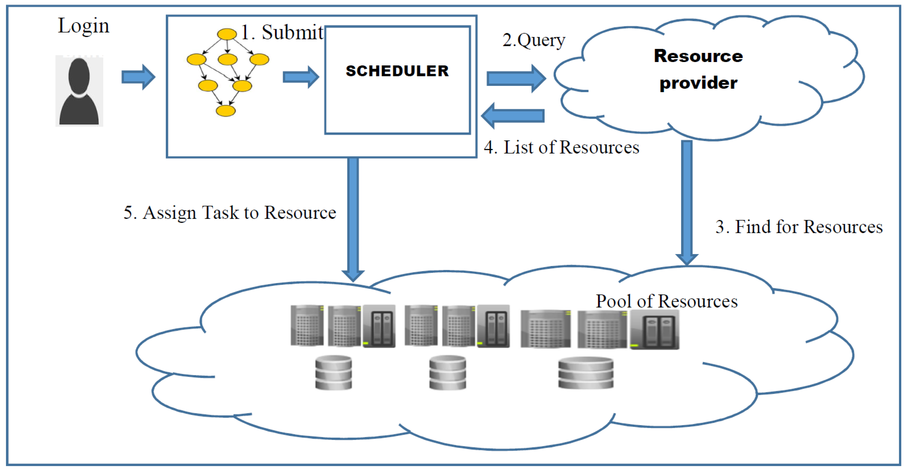
The workflow scheduling model has the following entities: user (denoted as ‘U’), scheduler (denoted as ‘S’), and resource provider (denoted as ‘RP’). The resource provider provides computational resources with various competencies. The cost and processing power information of the resources that are available is publicly published. The queries made by the scheduler related to the availability of resources are responded by the RP. The workflow application is submitted by the user to the scheduler in addition to the deadline (D) and budget (B). The execution of tasks in the workflow over the obtainable resources is decided by the scheduler. The entire flow of the workflow can be visualized in Figure 1.
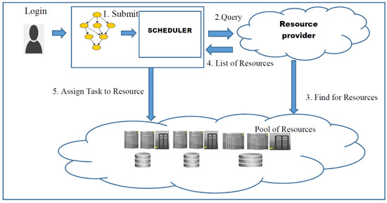
Figure 1.
Workflow scheduling model.
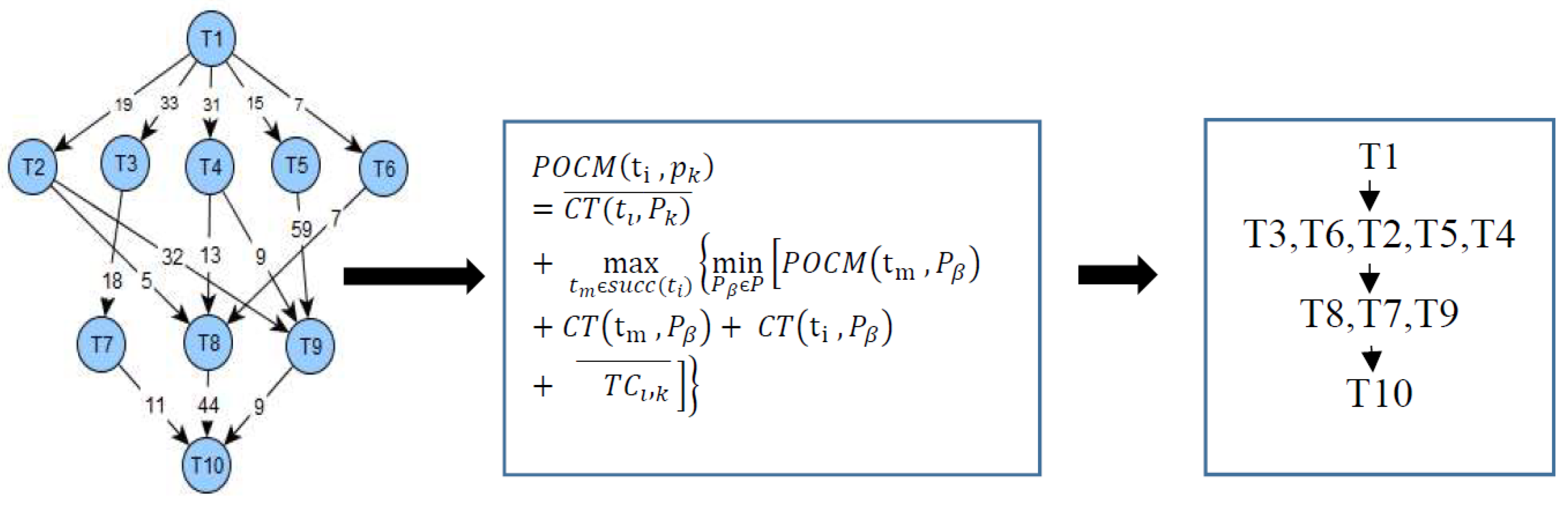
Figure 2 shows the rank computation model, where the workflow consists of tasks and is given as input to the workflow management system. The rank is calculated by using the predict optimal cost matrix. Based on the POCM, the task is prioritized, and the processor is selected to execute the tasks.
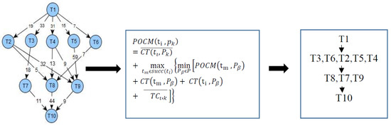
Figure 2.
Rank computation model.
3.3. Workflow Implementation Model
In Figure 2, the workflow implementation model of the offered method is shown. The DAG in the scientific workflows comprises nodes and edges. The edges signify data and control dependencies among the tasks, and the nodes signify distinct tasks that are being executed. The XML files of Workflowsim [24,25,26] consist of task files, and output data of one task can be given as input to another task. At the beginning, the location of the data and executables are not known to the workflow. A great number of workflow management systems (WMSs) use a similar kind of model. The WMSs are modeled using the Workflowsim tool, which can access immeasurable resources for lease depending on the system’s memory capacity. Some of the major components involved in the working of the workflow management system are given below.
- Workflow submission: In order to schedule the workflow tasks, the workflow application is submitted to the workflow management system (WMS) by the user. The host machine, such as users’ laptops or a public resource, can hold the WMS.
- Target implementation environment: This environment can be a well-known local host, such as a small user’s personal computer, it can be a cloud, such as a virtual environment like an AWS cloud, or it can be a physical cluster located at a remote place. Depending on the resource availability, the abstract workflow is mapped into the workflow in an executable form. WMS takes up the responsibility of monitoring the workflow execution. Moreover, it obtains the input, the output, and the files acquired during the course of execution of the workflow tasks. The major modules of the target implementation environment and their outline is as follows:
- ○
- Clustering engine: In the WMS the system overheads are decreased by grouping one or more relative small tasks into a job, which is a single execution unit.
- ○
- Workflow engine: As defined by the workflow, the single execution unit is called as jobs are submitted in sequence by the workflow engine as per the task dependencies. From the workflow engine, the jobs are given to the local workflow scheduling queue.
- ○
- Local queue and the local workflow scheduler: The individual workflow jobs are maintained and monitored by the workflow scheduler on both the remote and the local databases. The queuing delay is defined as the elapsed time on presenting the job to the job scheduler and the actual execution on the remote node.
- ○
- Remote implementation engine: The remote engine supervises the job execution on the remote compute nodes.
4. Proposed Algorithm
The rank is calculated based on the predict optimal cost matrix in the proposed algorithm, denotes the processor , and denotes the task . The rank calculation formula is given by
Here, = 0 when , and the value of for the exit task is .
The terms and are of great importance. The computation time denoted by defines the task importance of the current process on a processor , and defines the task importance of the successor node in the critical path. The aim of the algorithm is to allocate the task to the better processor, so that the makespan and the reduced cost is achieved. The existing algorithms have not considered the effect of task successors, but they just found the least EFT for a task and chose the processor accordingly.
The proposed method is shown in Algorithm 1. The algorithm has two stages. In phase one, prioritize that task; and in phase two, select the processor. In the prioritizing phase the tasks are ordered depending on the rank calculation in the reducing order. Rank is calculated as follows.
In the processor selection phase, two queues are maintained, namely the task queue and the ready queue. Initially, the task queue has all the tasks. Depending on the rank of the tasks, they move the task to the ready queue and calculate the earliest finish time of the processor and the VM cost at its earliest. Choose the processor with minimum EFT and cost. This process is repetitively done for all the tasks in the queue. Finally, the tasks with higher priority are mapped to the appropriate processor. The focus of this technique is to diminish the makespan and cost within the deadline and minimum cost.
4.1. Deadline and Budget Computation
The user-defined deadline is given as
where is the lowest time to execute and is the highest time to execute the application.
where is the parent task of in the critical path. is the deadline ratio between [0….1]. CP is the critical path of a DAG from tstart to tend.
is the highest time to execute the application.
is the minimum time required to execute on the fastest processor and is the maximum time to execute on the slowest processor.
= represents the lowest computation time to execute on the fastest processor. Where is the summation of computation time of all the task on the fastest processor.
represents the budget defined by the user, and it is given by
where is the budget ratio between [0….1], is the lowest cost to execute and the, which is the summation of the cost to execute a task on the critical path, and is the highest time to execute the application on the fastest processor, which is the summation of the cost to execute a task on the critical path.
is the cheapest cost involved in the execution of the application.
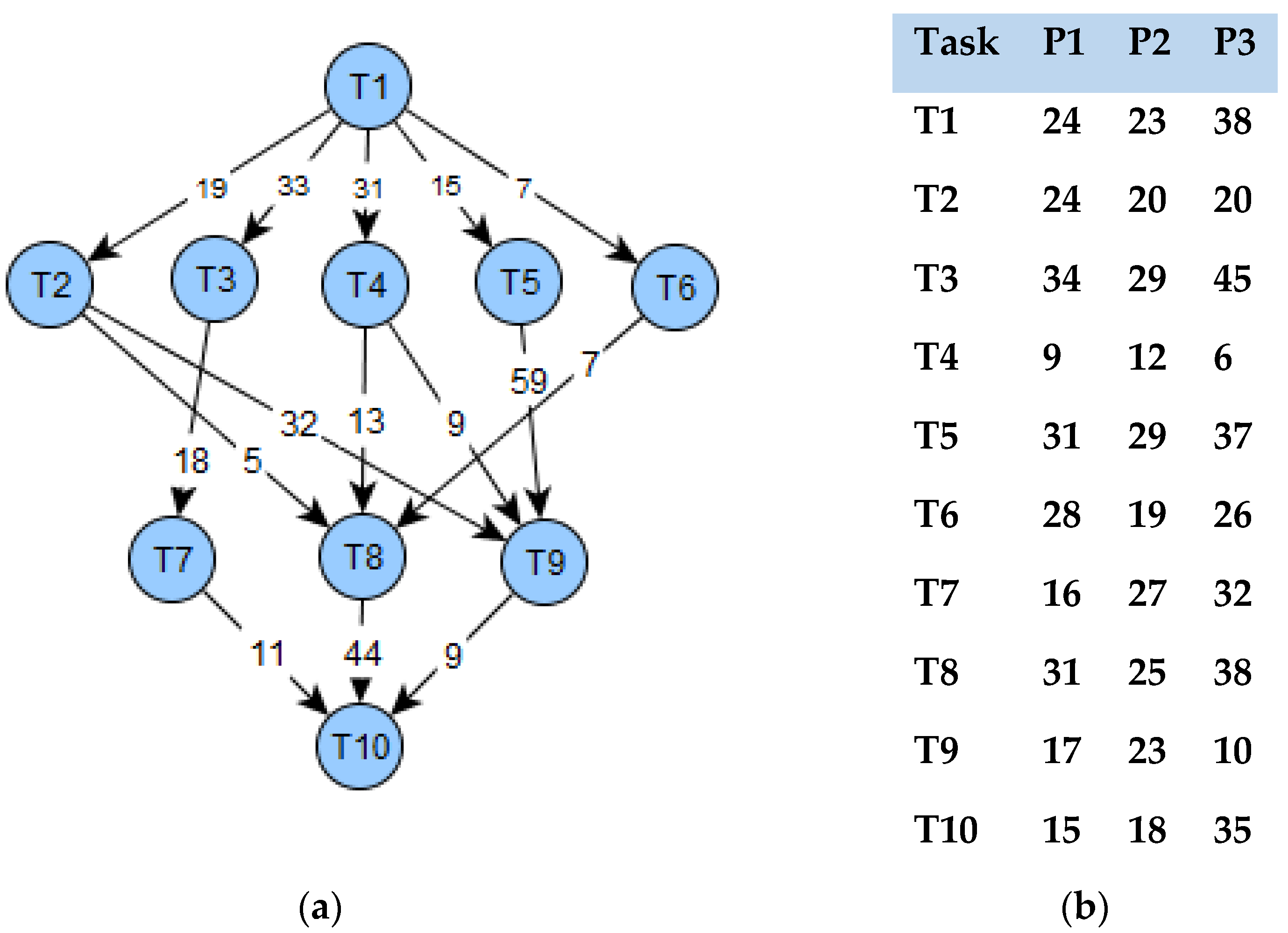
The critical path of Figure 3a is calculated as 1 → 4 → 8 → 10 which is 88.
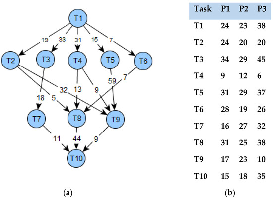
Figure 3.
(a) Sample DAG with the transfer cost of 10 tasks. (b) Computation cost of 10 tasks and 3 processors.
is the lowest execution cost of the task amid all the processors.
The initial deadline is given as . The sub-deadline of each level is calculated as
where SD denotes the sub-deadline of the task at each level. CT represents the computation time, and TC represents the transfer cost.
| Algorithm 1 POTC Planning Algorithm |
| Require: W = G (T,E) |
| Require: R =, and |
| 1. if D_user < CT_least and B_use < C_cheap |
| return no possible schedule |
| 2. Compute for all Tasks . |
| 3. Prioritize the task and list in decreasing order of Ranku |
| 4. Compute the sub deadline (SD) for all tasks |
| 5. Create an empty list in Ready Queue (RQ) |
| 6. Create tasks in the Task Queue (TQ) |
| 7. while TQ is < > do |
| 8. ← Assign highest rank task from TQ |
| 9. RQ ← Assign task and delete in TQ |
| 10. for all VM in the VM set Vj do |
| 11. Compute the Earliest Finish Time using |
| Assign task to Processor |
| 12. end for |
| 13. Update TQ |
| 14. End while |
| 15. Assign task ti to the VM Vj with Min Value |
4.2. Task Prioritization Phase
While prioritizing the task, consider one of the important tasks of the present task, which is nothing but its successor in the critical path node and the number of successors. For the DAG1, the cost matrix is shown in Figure 3a,b, while Table 1 shows the priority based on the matrix. The tasks’ priority list by is ordered as (T1, T3,T6,T2,T5,T4,T8,T7,T9,T10), the tasks’ priority list by is ordered as (T1,T5,T6,T2,T4,T3,T8,T7,T9,T10), and the tasks’ priority list by is ordered as (T1,T4,T6,T2,T3,T5,T8,T7,T9,T10). The ranking method can forecast the rank in the initial phase by considering the importance of a task’s relation, and the technique is similar to the rank calculation with . On comparing with we can see that include and which is similar to the [11] and method [13].

Table 1.
The rank obtained through the POCM, OCT, and upward rank for Figure 3.
4.3. Processor Selection Phase
After prioritizing the task, compute the Forecast EFT () for each task on a processor, which is defined by
After which, to execute a task, a processor that achieves the minimum is chosen. The main aim of the processor selection phase is to ensure that the descendants of the present task can complete its execution without an increase in complexity. The forecast method is explained as follows: consider the scheduling of task T1 and task T3: for the task T1, P2 is the resource that gives the least EFT, and for the task T3, P2 is the resource that gives the least EFT. Thus, T1 is scheduled to P2 and T2 is scheduled to P3. Moreover, for the entire DAG, the anticipated EFT is reduced. The makespan obtained from the proposed forecast-based algorithm is 114, the makespan obtained for the same DAG1 using PEFT is 134, and the makespan based on HEFT using the same DAG is 145. Thus, the obtained makespan using HEFT, PEFT, and POTC for the DAG1 is 145, 134, and 114.
The time complexity of the proposed method is calculated based on the rank computation and the task to resource mapping, Given the workflow with the number of tasks represented as ‘n’ and the dependencies represented as ‘e’. The first phase of the algorithm computes the rank of all the tasks which process the entire tasks and the edges. The time complexity of this step is given as . In the selection phase, the outer loop is for ‘n’ tasks and the inner loop is for ‘r’ resources. The time complexity for this phase is given as Thus, the final time complexity is given as. Thus, the time complexity of the proposed method is similar to PEFT, MOPT, and BDHEFT.
5. Results and Discussion
The results obtained by the POTC algorithm—along with the ELSH, MOPT, PEFT, and BDHEFT and their performance—are presented in this section. For the purpose of the experiment, two sets of workflow applications called ‘Epigenomics’ and ‘Montage’ were taken, and they represented the workflow real-world problems of genomics and astronomical Image Mosaic Engine. Firstly, the comparison metrics termed scheduling length ratio (SLR), for the proposed and existing algorithms were described.
Schedule Length Ratio (SLR):
This is one of the main measures of makespan (schedule length) of its output schedule. Schedule length ratio:
where Makespan [21] is the total implementation time, and signifies the minimum of the critical path. The denominator is the totality of all implementation costs of the tasks on the minimum critical path. Since the denominator is the lower bound, the schedule length ratio cannot be smaller than one. The performance of all three algorithms has been evaluated with some of the scientific workflows, namely Montage and Epigenomics. The total count of the tasks in each workflow is taken as Epigenomics: 30, 50, 100, 1000, and Montage: 30, 50, 100, and 1000. The simulation environment consists of a heterogeneous system with 20 virtual machines. The target system is generated based on ‘Workflowsim’, which is a Java framework.
Epigenomics: The average SLR results for Epigenomics are shown in Figure 4. The performance of the proposed algorithm using Epigenomics is shown in Figure 4. The average SLR shows 3.2% for 30 tasks, 3.29% for 50 tasks, 3.68% for 100 tasks, and 14.7% for 1000 tasks for the POTC algorithm. Thus, POTC for 50 tasks has improved by 6.4% over ELSH, and for 1000 tasks it has increased by 3.5%. In addition, POTC for 1000 tasks has improved by 6.9% over MOPT.
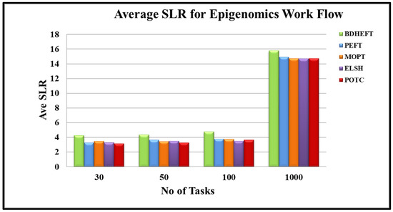
Figure 4.
Average schedule lengths ratio for the epigenome workflow.
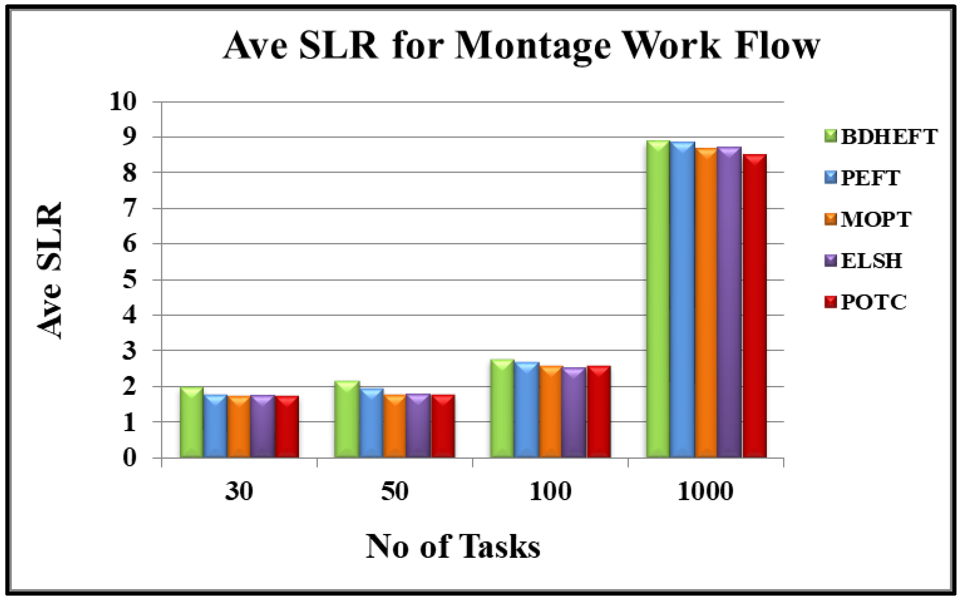
Montage: Figure 5 shows the average SLR of the real-world scientific workflow application Montage. Again, the POTC algorithm has shown a better performance when compared to the ELSH, MOPT, PEFT, and BDHEFT algorithms. Thus, for 30 tasks, POTC has improved its performance by 9.4% over MOPT, for 50 tasks POTC has improved its performance by 6.1% over MOPT, for 100 tasks POTC has improved its performance by 1.9% over MOPT, and for 1000 tasks POTC has improved its performance by 3.5% over MOPT, and thus POTC gives better performance over ELSH. Moreover, for 100 tasks, POTC has improved its performance by 30.4% over BDHEFT, and for 1000 tasks POTC has improved its performance by 11.3% over BDHEFT. Thus POTC, has a better performance than BDHEFT.

Figure 5.
Average schedule lengths ratio for the montage workflow.
Depending on these outcomes, with the results for DAG with a small and large task number, the POTC algorithm surpassed ELSH, MOPT, PEFT, and BDHEFT for both the Epigenomics and Montage workflow. For a huge graph, the POTC algorithm has a better performance. Table 2 shows how the processor is selected based on the rank and cost of various processors.
Table 2.
Selection of task and processor in each iteration of the algorithm.
Speedup: The speedup for any given graph is obtained by the division of the cumulative implementation time of the tasks in the graph by the length of the schedule. In other words, it is the sequential implementation time to the parallel implementation time. The sequential time is calculated by allocating all tasks to a single processor that reduces the implementation costs. If the total sum of the implementation costs is increased, it results in a larger speedup. Figure 6 shows the Speedup of the proposed algorithm compared with existing algorithms [27,28].
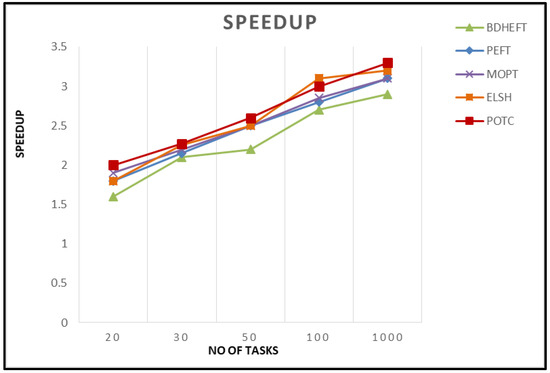
Figure 6.
Speedup comparison of the four algorithms.
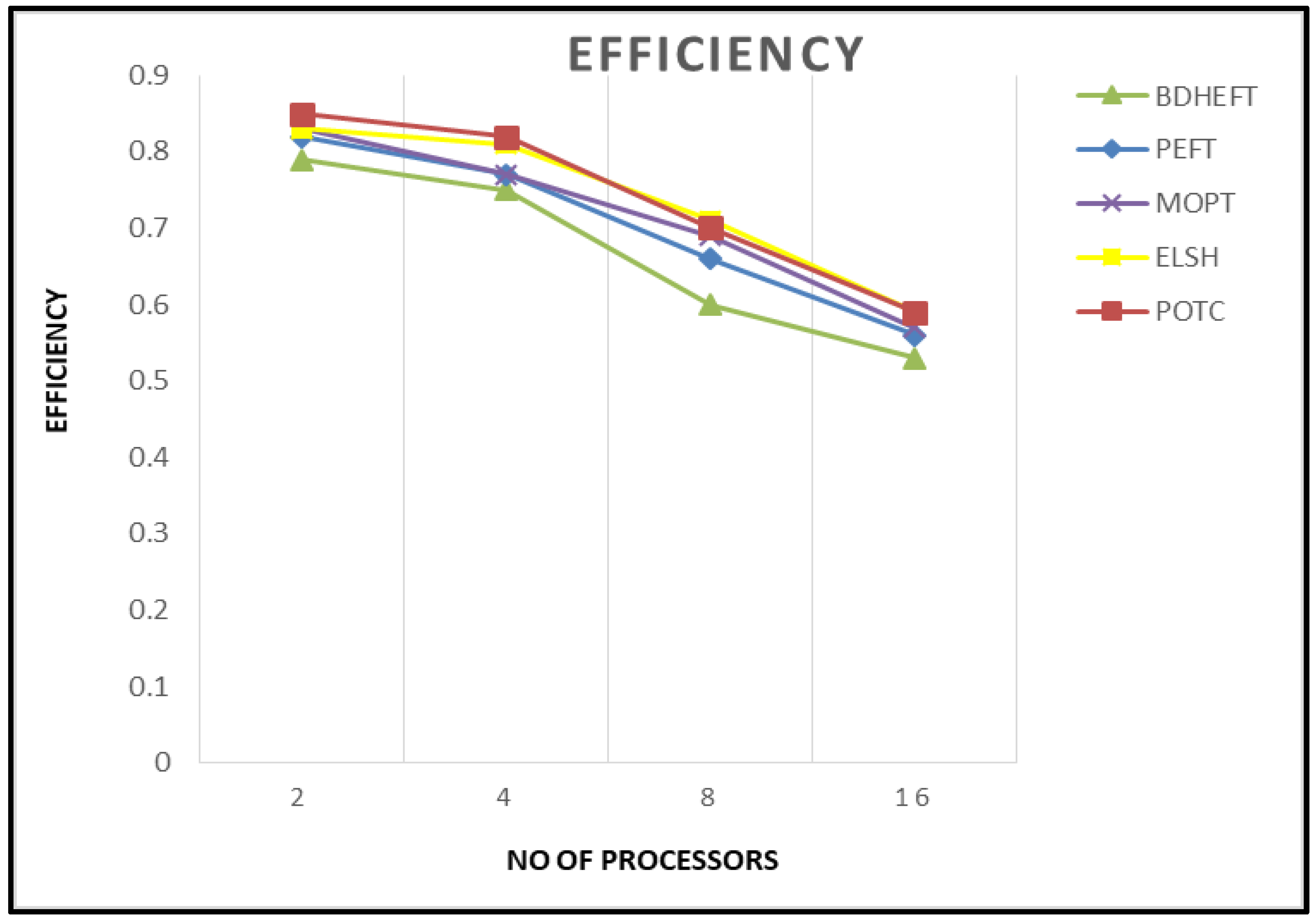
Efficiency: It is given by the ratio of speedup to the number of VMs used.
Figure 7 shows the efficiency of the BDHEFT, PEFT, MOPT, ELSH, and POTC algorithms. It shows that the performance of PEFT is very similar to that of MOPT. Higher values of efficiency are obtained by the proposed algorithm. For every algorithm, the makespan decreases as the number of processors is increased.
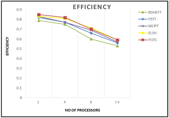
Figure 7.
Efficiency comparisons of the four algorithms.
Successful Rate: the successful rate is given as a ratio of the successful planning to the total number in the experiment.
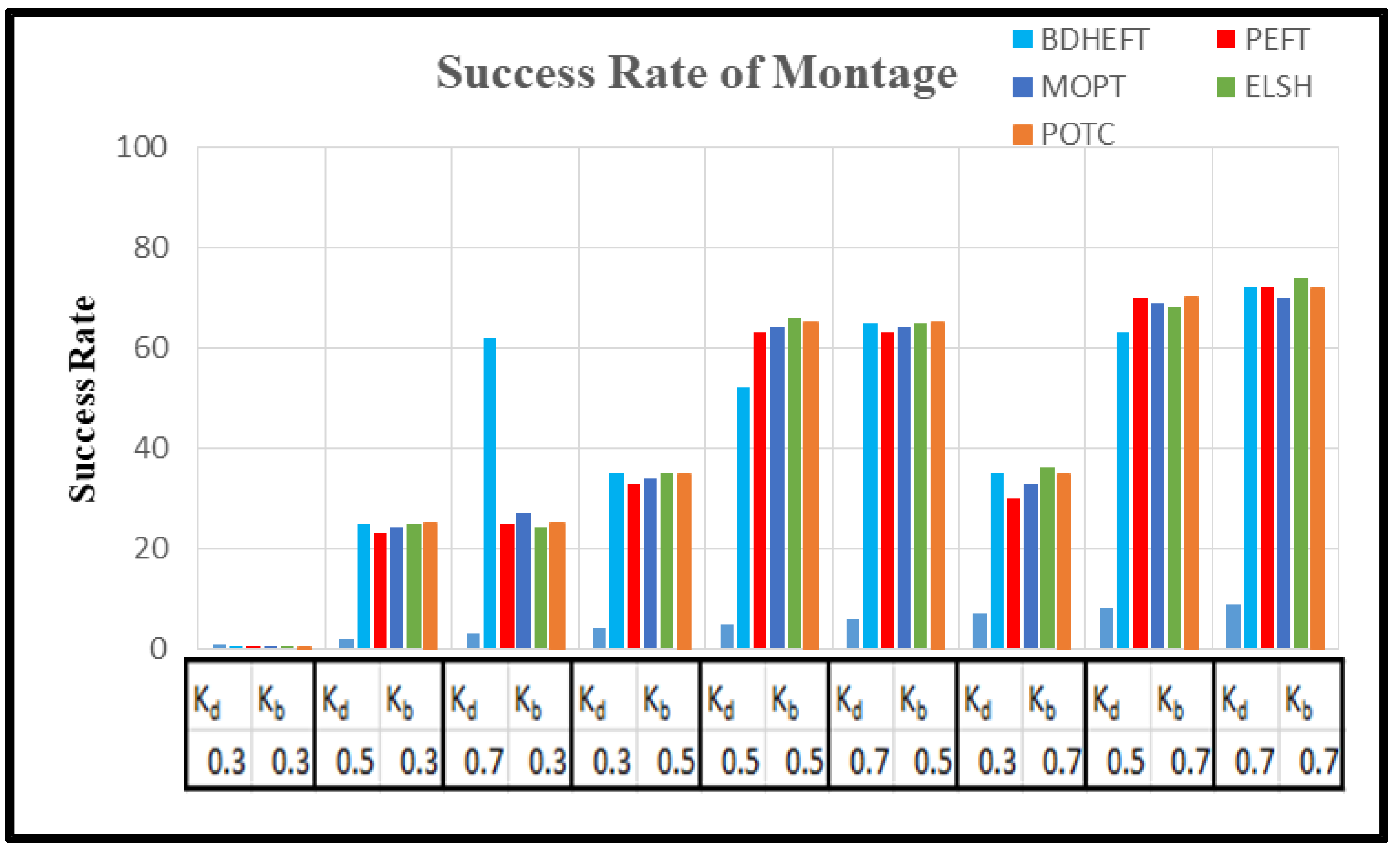
The graph of as in Equation (16) is captured with around 50 runs of simulations. The BDHEFT, PEFT, MOPT, ELSH, and POTC algorithms are selected for comparison. The processors that are supported by Workflowsim have processors with varying configurations, and their time and cost parameters vary. The deadline ratio () and Budget ratio ( values are considered as and . Some of the real-world applications, such as Epigenomics (I/O intensive workflow) and Montage (compute intensive workflow), are taken for analysis with 100 tasks, as shown in Figure 8 and Figure 9. Montage has a high communication to computation ratio [29,30,31], and epigenomics has a low communication to computation ratio . The success rate is always inversely proportional to. For Epigenomics, as shown in Figure 8, POTC has obtained a performance similar to those of MOPT and PEFT for the deadline (kd) = 0.7. The obtained performance using POTC is better when compared to BDHEFT for large budgets (kb).
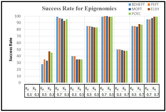
Figure 8.
Success rate of the epigenomics workflow.

Figure 9.
Success rate of the montage workflow.
Figure 9 shows the success rate of the montage workflow. PEFT, MOPT, ELSH, and POTC show a lower performance for lower values of budget (kb). The performance is similar to MOPT and ELSH for large values of the deadline (kd).
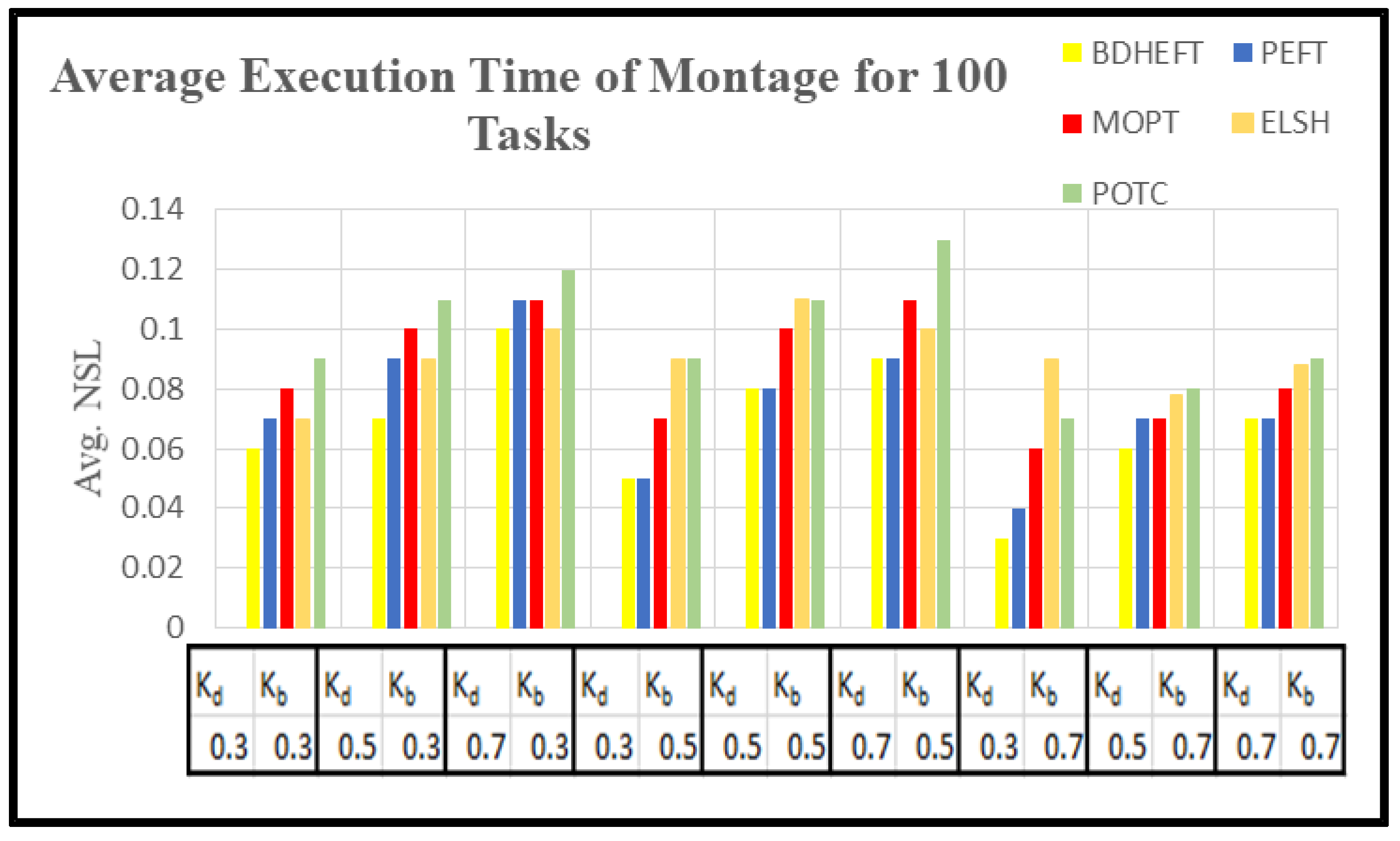
In order to compare the execution cost of various scientific workflows, we assume VMs of five different types with the processing speed of 1000–10,000 MIPS in a single data center. On the basis of the processing capacity, the task processing time was estimated. The cost varies between 2 and 10 units, and the time interval used in this tool is 1 h, which is similar to the Amazon cloud, which uses a pay-as-you go model. The metrics used to capture time and cost minimization are normalized schedule length (NSL) and normalized schedule cost (NSC) [32,33]. The NSL is defined by the ratio of the total execution time to the workflow execution time by executing them on the fastest resource.
where is the time required to execute the workflow tasks on the fastest resource.
is defined by the ratio of the total cost to the workflow execution cost by executing them on the cheapest resource.
where is the execution cost of the workflow while executing them on the cheapest resource.
Using 50 runs of simulations, both and are captured. Figure 10, Figure 11, Figure 12 and Figure 13 show the NSL and NSC of POTC-generated schedules with respect to ELSH, MOPT, PEFT, and BDHEFT. The deadline factors are set as 0.3, 0.5, and 0.7. The budget is relaxed by fixing the deadline and varying the budget for different values of = 0.3, 0.5, and 0.7. To assign the workflow tasks, the scheduler chooses the fastest or the expensive resources. Thus, for the created schedule under the same deadline, tends to increase with the decrease in [34].

Figure 10.
Average execution time of the montage workflow for different deadline factors.
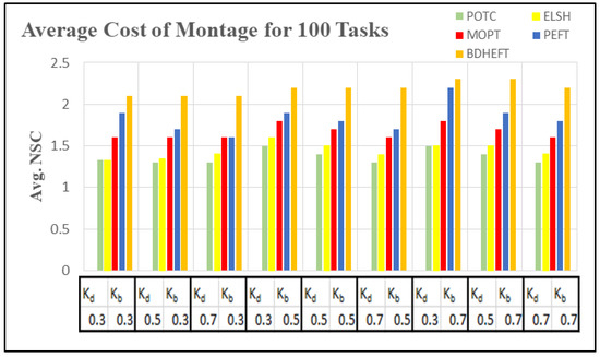
Figure 11.
Average execution cost of the montage workflow for different deadline factors.
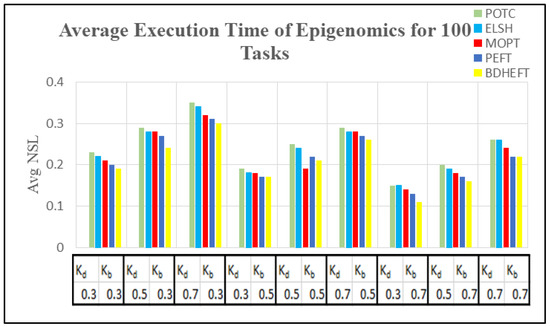
Figure 12.
Average execution time of the epigenomics workflow for different deadline factors.
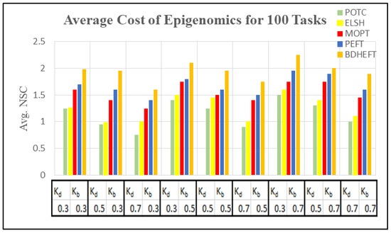
Figure 13.
Average execution cost of the epigenomics workflow for different deadline factors.
Figure 10 and Figure 12 show the average execution times of the Montage and Epigenomics workflows, and Figure 11 and Figure 13 show the average execution costs of the Montage and Epigenomics workflows. As the value of increases, the execution cost decreases and increases. When budget () is fixed, the deadline is relaxed by varying the deadline from 0.3 to 0.7. Subsequently, the inexpensive or the slowest resources are chosen by the scheduler. Thus, under the same budget, is minimized and the of the workflow decreases as shown in Figure 9, Figure 10, Figure 11 and Figure 12. Furthermore, by varying the budget ratio and the fixed deadline, for each of these values, the budget is relaxed. Now according to the user preference, the scheduler is able to choose the fastest resource or the inexpensive resource.
From the above results, it has been found that the average cost of the proposed method is minimized for montage by 7.1% and about 3.2% more for makespan with respect to BDHEFT. For the Epigenomics workflow, the average cost is minimized by 8.3%, with about 4.1% more for makespan. The overall results show that the proposed method (POTC) outperforms ELSH, MOPT, PEFT, and BDHEFT under the same budget and deadline by minimizing the average cost while improving the makespan, similar to the one given by BDHEFT. Thus, this method can handle various workflow applications of Amazon EC2 instances with varying capacities and cost.
6. Conclusions
In this article, the Predict Optimistic Time and Cost (POTC) algorithm has been proposed for scheduling scientific workflows onto heterogeneous systems more effectively. The proposed algorithm is tested with some of the real-world scientific workflows, namely the Epigenomics and Montage workflows. The proposed POTC algorithm has significantly outperformed the other existing algorithms, namely ELSH, MOPT, PEFT, and BDHEFT, in terms of performance metrics and cost metrics, such as schedule length ratio, speedup, efficiency, and normalized schedule cost. The main contribution of this proposed algorithm is the introduction of ranking before scheduling and performing the execution of tasks based on ranks which are based on cost and time. In addition to ranking the scheme and processor selection scheme, the deadline and budget are also considered in this work to improve the speed of the overall execution of tasks. From the experiments conducted in this work, it is proven that the proposed ranking scheme minimizes the processing time and cost and assigns the best processors for each of the tasks. Instead of considering only the earliest finish time, the selection phase also considered the processor with minimum cost for executing the task. All processors are tested, and the processor which takes minimum time and minimum cost is selected in this algorithm. Moreover, the forecast feature has been proposed in the algorithm while maintaining the same quadratic complexity. The proposed POTC algorithm outclassed all other scheduling algorithms with respect to the scheduling length ratio and cost. Statistically, POTC has the lowest average schedule length ratio, the lowest cost, and better speedup and efficacy. Thus, considering the results, it is concluded that for the DAGs in a heterogeneous environment, the proposed static scheduling algorithm named POTC exhibits an improved performance.
In the future, more experiments based on the various real workflows with many characteristics can be conducted. Energy consumption is also one of the crucial user requirement in clouds. As a future study, we plan to integrate this objective in the proposed algorithm. We are also interested in implanting this algorithm onto hybrid cloud platforms in addition to edge-cloud computing systems.
Author Contributions
Conceptualization, J.H.; Methodology, J.H. and S.C.; Supervision, S.C.; Writing–original draft, J.H. All authors have read and agreed to the published version of the manuscript.
Funding
This research received no external funding.
Data Availability Statement
Not Applicable, the study does not report any data.
Conflicts of Interest
No conflict of interest.
References
- Singh, V.; Gupta, I.; Jana, P.K. A novel cost-efficient approach for deadline-constrained workflow scheduling by dynamic provisioning of resources. Futur. Gener. Comput. Syst. 2018, 79, 95–110. [Google Scholar] [CrossRef]
- Tan, W.; Zhou, M. Business and Scientific Workflows: A Web Service-Oriented Approach; John Wiley & Sons: Hoboken, NJ, USA, 2013; Volume 5. [Google Scholar]
- Bagheri, R.; Jahanshahi, M. Scheduling Workflow Applications on the Heterogeneous Cloud Resources. Indian J. Sci. Technol. 2015, 8, 1. [Google Scholar] [CrossRef]
- Arabnejad, V.; Bubendorfer, K.; Ng, B. Deadline distribution strategies for scientific workflow scheduling in commercial clouds. In Proceedings of the 2016 IEEE/ACM 9th International Conference on Utility and Cloud Computing (UCC), Shanghai, China, 6–9 December 2016; IEEE: New York, NY, USA, 2017; pp. 70–78. [Google Scholar]
- Yang, T.; Gerasoulis, A. DSC: Scheduling parallel tasks on an unbounded number of processors. IEEE Trans. Parallel Distrib. Syst. 1994, 5, 951–967. [Google Scholar] [CrossRef] [Green Version]
- Ranaweera, S.; Agrawal, D.P. A task duplication based scheduling algorithm for heterogeneous systems. In Proceeding of the 14th International Parallel and Distributed Processing Symposium. IPDPS 2000, Cancun, Mexico, 1–5 May 2000; IEEE: New York, NY, USA, 2002; pp. 445–450. [Google Scholar]
- Lal, A.; Krishna, C.R. A review on methodologies of scientific workflow scheduling algorithm under dead line constraint. In Proceeding of the 2017 International Conference on Energy, Communication, Data Analytics and Soft Computing (ICECDS), Chennai, India, 1–2 August 2017; IEEE: New York, NY, USA, 2017; pp. 3533–3536. [Google Scholar]
- Arabnejad, V.; Bubendorfer, K. Cost effective and deadline constrained scientific workflow scheduling for commercial clouds. In Proceeding of the 2015 IEEE 14th International Symposium on Network Computing and Applications, Cam-bridge, MA, USA, 28–30 September 2015; IEEE: New York, NY, USA, 2016; pp. 106–113. [Google Scholar]
- Arunarani, A.; Manjula, D.; Sugumaran, V. Task scheduling techniques in cloud computing: A literature survey. Futur. Gener. Comput. Syst. 2019, 91, 407–415. [Google Scholar] [CrossRef]
- Lee, Y.C.; Han, H.; Zomaya, A.; Yousif, M. Resource-efficient workflow scheduling in clouds. Knowl. Based Syst. 2015, 80, 153–162. [Google Scholar] [CrossRef]
- Topcuoglu, H.; Hariri, S.; Wu, M.-Y. Performance-effective and low-complexity task scheduling for heterogeneous computing. IEEE Trans. Parallel Distrib. Syst. 2002, 13, 260–274. [Google Scholar] [CrossRef] [Green Version]
- Verma, A.; Kaushal, S. Cost-Time Efficient Scheduling Plan for Executing Workflows in the Cloud. J. Grid Comput. 2015, 13, 495–506. [Google Scholar] [CrossRef]
- Arabnejad, H.; Barbosa, J. List Scheduling Algorithm for Heterogeneous Systems by an Optimistic Cost Table. IEEE Trans. Parallel Distrib. Syst. 2014, 25, 682–694. [Google Scholar] [CrossRef]
- Djigal, H.; Feng, J.; Lu, J. Task Scheduling for Heterogeneous Computing using a Predict Cost Matrix. In Proceedings of the 48th International Conference on Parallel Processing: Taskshops, Kyoto, Japan, 5–8 August 2019; ACM: New York, NY, USA, 2019; p. 25. [Google Scholar]
- Bittencourt, L.F.; Sakellariou, R.; Madeira, E.R. Dag scheduling using a lookahead variant of the heterogeneous earliest finish time algorithm. In Proceedings of the 2010 18th Euromicro Conference on Parallel, Distributed and Network-Based Processing, Pisa, Italy, 17–19 February 2010; IEEE: New York, NY, USA, 2009; pp. 27–34. [Google Scholar]
- Zhou, N.; Qi, D.; Wang, X.; Zheng, Z.; Lin, W. A list scheduling algorithm for heterogeneous systems based on a critical node cost table and pessimistic cost table. Concurr. Comput. Pr. Exp. 2016, 29, e3944. [Google Scholar] [CrossRef]
- Ijaz, S.; Munir, E.U. MOPT: List-based heuristic for scheduling workflows in cloud environment. J. Supercomput. 2018, 75, 3740–3768. [Google Scholar] [CrossRef]
- Wu, Q.; Zhou, M.; Wen, J. Endpoint Communication Contention-Aware Cloud Workflow Scheduling. IEEE Trans. Autom. Sci. Eng. 2021, 1–14. [Google Scholar] [CrossRef]
- Zhang, P.; Zhou, M. Dynamic Cloud Task Scheduling Based on a Two-Stage Strategy. IEEE Trans. Autom. Sci. Eng. 2018, 15, 772–783. [Google Scholar] [CrossRef]
- Hu, B.; Cao, Z.; Zhou, M. Energy-Minimized Scheduling of Real-Time Parallel Workflows on Heterogeneous Dis-tributed Computing Systems. IEEE Trans. Serv. Comput. 2021. Available online: https://researchwith.njit.edu/en/publications/energy-minimized-scheduling-of-real-time-parallel-workflows-on-he (accessed on 9 October 2021).
- Van den Bossche, R.; Vanmechelen, K.; Broeckhove, J. Online cost-efficient scheduling of deadline-constrained taskloads on hybrid clouds. Future Gener. Comput. Syst. 2013, 29, 973–985. [Google Scholar] [CrossRef]
- Zhou, X.; Zhang, G.; Sun, J.; Zhou, J.; Wei, T.; Hu, S. Minimizing cost and makespan for workflow scheduling in cloud using fuzzy dominance sort based HEFT. Futur. Gener. Comput. Syst. 2019, 93, 278–289. [Google Scholar] [CrossRef]
- Li, Z.; Ge, J.; Yang, H.; Huang, L.; Hu, H.; Hu, H.; Luo, B. A security and cost aware scheduling algorithm for heterogeneous tasks of scientific workflow in clouds. Futur. Gener. Comput. Syst. 2016, 65, 140–152. [Google Scholar] [CrossRef]
- Chen, W.; Deelman, E. Workflowsim: A toolkit for simulating scientific workflows in distributed environments. In Proceedings of the 2012 IEEE 8th International Conference on E-Science, Chicago, IL, USA, 8–12 October 2012; IEEE: New York, NY, USA, 2012; pp. 1–8. [Google Scholar]
- Hilda, J.; Srimathi, C. Coupling Factor and Cost Based Task Clustering Method to Optimize Task Clustering for Scientific Workflows in Cloud Environment. Int. J. Eng. Adv. Technol. 2019, 4136–4143. Available online: https://www.ijeat.org/wp-content/uploads/papers/v8i6/F9288088619.pdf (accessed on 9 October 2021).
- Chakravarthi, K.K.; Shyamala, L.; Vaidehi, V. Cost-effective workflow scheduling approach on cloud under deadline constraint using firefly algorithm. Appl. Intell. 2021, 51, 1629–1644. [Google Scholar] [CrossRef]
- Ahmad, W.; Alam, B.; Ahuja, S.; Malik, S. A dynamic VM provisioning and de-provisioning based cost-efficient deadline-aware scheduling algorithm for Big Data workflow applications in a cloud environment. Clust. Comput. 2021, 24, 249–278. [Google Scholar] [CrossRef]
- Zheng, W.; Qin, Y.; Bugingo, E.; Zhang, D.; Chen, J. Cost optimization for deadline-aware scheduling of big-data processing jobs on clouds. Futur. Gener. Comput. Syst. 2018, 82, 244–255. [Google Scholar] [CrossRef]
- Pan, Y.; Wang, S.; Wu, L.; Xia, Y.; Zheng, W.; Pang, S.; Zeng, Z.; Chen, P.; Li, Y. A Novel Approach to Scheduling Workflows Upon Cloud Resources with Fluctuating Performance. Mob. Networks Appl. 2020, 25, 690–700. [Google Scholar] [CrossRef]
- Khalili, A.; Babamir, S.M. Optimal scheduling workflows in cloud computing environment using Pareto-based Grey Wolf Optimizer. Concurr. Comput. Pr. Exp. 2017, 29, e4044. [Google Scholar] [CrossRef]
- Kaur, A.; Singh, P.; Batth, R.S.; Lim, C.P. Deep-Q learning-based heterogeneous earliest finish time scheduling algorithm for scientific workflows in cloud. Software: Pr. Exp. 2020. [Google Scholar] [CrossRef]
- Han, P.; Du, C.; Chen, J.; Du, X. Minimizing Monetary Costs for Deadline Constrained Workflows in Cloud Environments. IEEE Access 2020, 8, 25060–25074. [Google Scholar] [CrossRef]
- Sujana, J.A.J.; Revathi, T.; Rajanayagam, S.J. Fuzzy-based Security-Driven Optimistic Scheduling of Scientific Workflows in Cloud Computing. IETE J. Res. 2018, 66, 224–241. [Google Scholar] [CrossRef]
- Chen, W.; Xie, G.; Li, R.; Li, K. Execution cost minimization scheduling algorithms for deadline-constrained parallel applications on heterogeneous clouds. Clust. Comput. 2021, 24, 701–715. [Google Scholar] [CrossRef]


Publisher’s Note: MDPI stays neutral with regard to jurisdictional claims in published maps and institutional affiliations. |
© 2021 by the authors. Licensee MDPI, Basel, Switzerland. This article is an open access article distributed under the terms and conditions of the Creative Commons Attribution (CC BY) license (https://creativecommons.org/licenses/by/4.0/).