Article

Performance Model for Video Service in 5G Networks

1
Department of Electrical and Computer Engineering, University of Massachusetts, Lowell, MA 01854, USA
2
Graduate School of Science and Engineering, Altinbas University, 34217 Istanbul, Turkey
3
Q Factor Communications, 255 Bear Hill Road, Waltham, MA 02451, USA
*
Author to whom correspondence should be addressed.
Future Internet 2020, 12(6), 99; https://doi.org/10.3390/fi12060099
Submission received: 25 April 2020 / Revised: 4 June 2020 / Accepted: 4 June 2020 / Published: 8 June 2020
(This article belongs to the Special Issue Future Networks: Latest Trends and Developments)

Abstract

:
Network slicing allows operators to sell customized slices to various tenants at different prices. To provide better-performing and cost-efficient services, network slicing is looking to intelligent resource management approaches to be aligned to users’ activities per slice. In this article, we propose a radio access network (RAN) slicing design methodology for quality of service (QoS) provisioning, for differentiated services in a 5G network. A performance model is constructed for each service using machine learning (ML)-based approaches, optimized using interference coordination approaches, and used to facilitate service level agreement (SLA) mapping to the radio resource. The optimal bandwidth allocation is dynamically adjusted based on instantaneous network load conditions. We investigate the application of machine learning in solving the radio resource slicing problem and demonstrate the advantage of machine learning through extensive simulations. A case study is presented to demonstrate the effectiveness of the proposed radio resource slicing approach.

1. Introduction

Fifth generation (5G) cellular networks are required to support cell capacity of multi-gigabit per second (Gbps) and cell edge throughput of tens of megabits per second (Mbps). In addition to the pure performance metrics, such as the rate, latency, reliability, and allowed connections, the scope of 5G incorporates the transformation of the mobile network ecosystem and accommodates heterogeneous services using one infrastructure [1]. To achieve this goal, 5G networks incorporate a technique named network slicing. Network slicing tries to slice the whole network into slices, each of which is tailored to the specific service requirements that are agreed to in a service level agreement (SLA) with customers (also known as tenants). Therefore, network slicing is an emerging business for operators that allows them to sell the customized network slices to various tenants at different prices [1]. As part of network slicing, radio access network (RAN) slicing defines a shared RAN connected to each of the multiple tenants’ core networks, with radio resources distributed by the central controller to different tenants, to maximize the radio resource usage.
To provide better-performing and cost-efficient services, RAN slicing is looking to intelligent radio resource management approaches to be aligned with users’ activities per slice. For radio access networks, the spectrum is expensive; thus, guaranteeing high spectrum efficiency (SE) is meaningful. SLAs usually impose stringent requirements on the network quality of services (QoS). Therefore, it is critical to investigate how to intelligently respond to the dynamics of the traffic load from mobile users to obtain satisfactory QoS in each slice at an acceptable spectrum cost [1]. In particular, RAN providers must implement new radio resource management approaches to map incoming SLA requirements associated with network slice requests into physical resources. Because of the implementation complexity, there is no explicit relationship between SLA requirements and physical resources to fulfill a service’s QoS requirements. Furthermore, 5G networks are expected to provide diverse QoS guarantees for a wide range of services with various requirements. Therefore, there is increased difficulty in translating user-friendly business terms into resource-specific attributes in the 5G network.
Considering these problems, we propose an approach to map customer-friendly business requirements to network attributes and achieve QoS assurance as part of the 5G RAN network design solution. Data analytics and machine learning (ML) using regression algorithm allow automated identification of relationships and dependencies between different parameters. For that reason, such approaches are exploited in the context of SLA mapping, given the need to correlate input parameters (high-level SLA requirements) with output parameters (i.e., low-level network attributes) [2]. For the QoS requirements specified in the SLA, a corresponding performance model can be provided. In this paper, the QoS performance model defines mapping between SLA high-level requirements and low-level network attributes. A performance model is constructed for each service, optimized using interference coordination approaches, and used to facilitate the network design and optimization process.
We propose interference coordination (IC) approaches to optimize the constructed QoS performance model. There are static and dynamic IC approaches. The static IC approaches include conventional fractional frequency reuse, which splits and distributes the spectrum among neighbor sectors [3,4,5]; partial frequency reuse, which splits the spectrum into two segments, one segment used for the cell edge user equipment (UEs) has a frequency reuse factor larger than one, and the other segment used for the cell center UEs has a frequency reuse factor of one [6,7]; and soft frequency reuse, which splits the spectrum into N segments, one prioritized segment is used with higher transmit power for edge UEs, and other segments are used with lower transmit power for central UEs, and prioritized segments of neighbor cells are orthogonal in frequency [8,9,10,11]. Dynamic IC approaches include IC approaches in frequency domain (FIC) and in time domain (TIC). Carrier aggregation-based IC [12,13] is a dynamic FIC approach, which defines primary component carrier (PCC) and secondary component carrier (SCC): each cell allocates one PCC for call setup and control channel transmission, etc., and dynamically allocates SCCs, according to the traffic load, SCC selection algorithms are used to optimize the system throughput. The almost blank subframe approach is a dynamic TIC approach that allows time-sharing of the spectrum [14,15,16]. The cell causing interference mutes some subframes so that interfered cells can serve their UEs. These subframes are “almost blank” because broadcast signals are still transmitted over the subframes.
For the above IC approaches, the sharing of time and frequency resources can be designed using graph- or utility-based approaches. The graph-based IC approaches (GIC) mitigates inter-cell interference by partitioning an interference graph, its nodes represent the UE and its edges represent the interference between UEs. The approach avoids the same time or frequency resources to be allocated to connected UEs to achieve a desired minimum signal-to-interference-plus-noise ratio (SINR) [17,18,19]. Utility-based IC (UIC) approaches maximize utility over the network [20,21,22,23]. A two-level approach has been proposed in [21,22,23]: at the sector level, each sector calculates utilities for scenarios with a different number of interferers; at central level, a central unit allocates resources for sectors and resolves interferers’ conflicts according to calculated utilities at the sector level.
Millimeter-waves (mmWave) occupy the frequency spectrum between 30 GHz and 300 GHz, offer a solution for 5G networks because of the vast amounts of spectrum [24], and the small wavelength that enables the realization of massive MIMO antenna arrays in small sizes. By using massive MIMO antenna arrays, two IC approaches—coordinated beamforming (CBF) and coordinated multi-user MIMO (MU-MIMO)—were proposed. Precoding matrix indicator (PMI) coordination is a lightweight CBF approach, in which each UE transmits “restriction PMI” or “recommendation PMI,” and its neighboring base stations (BTS) can either avoid using the restriction PMI or use the recommendation PMI [25]. For coordinated MU-MIMO schemes, a virtual transmitter has been formed by nearby cells to perform MU-MIMO transmission toward UEs, to eliminate inter-cell interference and achieve the highest cell capacity [26,27].
Beamforming systems include switched beam systems (SBSs) and adaptive array systems (AASs). Switched beam system uses fixed beams and beam patterns to point to predetermined directions within a cell [28]. Adaptive array system forms a beam pattern for each user, the beam pattern is generated to direct the main lobe to the desired UE and nulls to interfered UEs for interference suppression [29]. The motivation for an SBS is its lower cost, as AAS is expensive for commercial mobile networks.

Contribution

In this paper, we present a two-level dynamic IC approach, referred to as intra-cluster and inter-cluster levels, coordinated in the time and frequency domains, to construct and optimize the QoS performance model, and an approach for utilizing the constructed QoS performance model for network design and optimization. The approach targets the SBS on the mmWave band, employs MU-MIMO to improve the system capacity, and is designed for delay-sensitive traffic (i.e., video services, which are fixed wireless access applications (FWA)). The main contributions of this paper include the following:
  • Our proposed approach targets improvement in performance models that map high-level customer-friendly business requirements to low-level network parameters and achieve QoS assurance for delay-sensitive traffic.
  • The data analytics and ML approach is employed to construct the QoS performance model for network design and optimization, to identify the relationships and dependencies between SLA high-level requirements and low-level network attributes.
The paper is organized as follows: the problem is formulated in Section 2, the proposed approach is described in Section 3, the simulation methodology is described in Section 4, the simulation results are presented in Section 5, the complexity analysis is shown in Section 6, and Section 7 concludes the paper.

2. Problem Description

By balancing the relative importance of resource utilization (i.e., SE) and the quality of experience (QoE) satisfaction ratio, the resource management problem could be formulated as R = α · SE +   β   · QoE, where α and β represent the weights of SE and QoE [1]. QoE is subjective, so we use QoS instead.
Consider an area with U users, denoted as U = { 1 ,   ,   U } , uniformly distributed within the area, supporting S services, denoted as S = { 1 ,   ,   S } , and sharing the aggregated bandwidth W. Denote U s as users supporting service s . Due to the lack of physical resources, sites are shared among services, and are uniformly distributed within the area (with the same inter-site distance (ISD) between the sites). In a real network, instead of maximizing QoS, maximizing the number of users who satisfy the QoS requirements is the target. The problem is written as:
Problem SM-P1:
M a x i m i z e   [ α   ·   SE ( w , i s d ) +   β   · s S u U s N ( q o s u ( w , i s d ) ) ]
Over: w , i s d , where:
w = ( w 1 ,     w s ) N ( q o s u ( w , i s d ) ) = { 1 q o s u ( w , i s d ) > T s 0 E l s e
Subject to:
s S w s = W
where T s is the pre-defined threshold for service S. q o s u ( w , i s d ) > T s tells us that the QoS requirement T s of service s is satisfied by user u under network attributes, such as the bandwidth distribution of w and the site separation of i s d .
To address the complexity, a sub-optimal solution is proposed to put higher priority on the QoS requirement, optimize radio resource utilization using IC approach, and allocate dedicated bandwidth for each service. The proposed solution includes two steps. First, create a performance model for each service. The problem can be transferred into solving the following performance model over different w s and i s d :
P M s ( w s , i s d ) = u U s N ( q o s u ( w s , i s d ) )
Second, perform an exhaustive search in the ISD space and W space for all services. The point satisfied the total bandwidth constraint and fulfills the QoS requirements for all services yet with the maximized ISD, is the optimized solution.
The core of the solution is solving the performance model for each service. Data analytics and machine learning approaches using regression algorithm that allow automated identification of non-explicit relationships and dependencies are exploited. With the performance model, the following problems are investigated: (1) optimization of the performance model using IC approaches, (2) network design using the performance models, and (3) network optimization.
In this research, the proposed UIC approaches are on both time (TIC) and frequency (FIC) domains. First, we modify the approach we proposed in [29], extend it into the time domain, and apply the approach to the video service. Assume the mobile network consists of C cells, denoted as C = { 1 ,   ,   C } , U users, denoted as U = { 1 ,   ,   U } , and B sub-bands, denoted as B = { 1 ,   ,   B } . Consider a SBS network with M beams per sector, denoted as M = { 1 ,   ,   M } , and T transmission time intervals (TTIs) per scheduling period, denoted as T = { 1 ,   ,   T } . Define I b u , c , m ( t ) as user resource allocation indicator which indicates that if I b u , c , m ( t ) = 1, the cell c will transmit to the user u using the beam m on the sub-band b at time t. Otherwise, I b u , c , m ( t ) = 0; define U c as the group of users served by the cell c. Define I c ( t ) = { I b u , c , m ( t ) : u U c ,   m M ,   b B } , I ( t ) = { I c ( t ) :   c C } . Define p b u , c , m ( t ) as the power transmitted by the cell c using the beam m on the sub-band b to the user u at time t. Define p ( t ) = { p b u , c , m ( t ) : u U , c C , m M ,   b B } .
This research assumes an SBS system using basic and switched directional antennas. Each user chooses one beam to transmit, referred as the serving beam, and we define the strongest beam from cell c to user u as m ˜ u , c . We also assume a constant transmit power p 0 per sub-band for each cell. If multiple beams are transmitted, the power will be distributed evenly among the simultaneously transmitted beams. The following Figure 1, Figure 2, and Equations (6)–(8) describe the assumptions.
Figure 1 shows the radiation pattern of basic and switched directional antennas with 15 ° ,   30 ° , and 60 ° of half power beam width (HPBW), denoted as θ B . Equation (6) shows the radiation pattern in decibels [30], where G 0 , d B is the maximum gain and G , d B is the averaged gain values at the sidelobe.
G t ( ) = { G 0 ,   d B 12 ( θ B ) 2 | |   1.3 * θ B G , d B | | > 1.3 * θ B
p b u , c , m = p 0 u 1 U c ,   m 1 M I u 1 , c , m 1 *   G t ( u , c , m )
where u , c , m is calculated by:
u , c , m = cos 1 ( u c ) ·   m | u c | | m |
u and c are the location vectors of the user and the cell, m is the direction vector of the beam boresight, shown in Figure 2 [29].
With the above assumptions, the optimization problem is written as a function of I , u ,   c   , and m :
Problem IC-P1:
u , c , m = cos 1 ( u c ) ·   m | u c | | m |
M a x i m i z e t T b B c C u U c w u m M r b u , c , m ( I )
Over: I
Subject to:
I b u , c , m ( t ) = { 1       m = m ˜ u , c 0       E l s e
u c   I b u , c , m ( t )   M m a x         c C ,   t T , b B
where
r b u , c , m ( I ) = W log 2 [ 1 + S I N R b u , c , m ( I ) ]
where
S I N R b u , c , m ( I ) = g u , c   p b u , c , m l C , k M ,   ( l c & k m )   I b u , l , k *   g u , l *   p b u , l , k + σ b u .
p b u , c , m is defined in Equations (6)–(8). w u is the weight of user u. For video traffic, w u is calculated using the head of line delay of the video traffic. W is the bandwidth. g u , c is the channel gain, which depends on the distance between the cell c and the user u. M m a x is the maximum number of beams per cell. σ b u is the thermal noise.
Problem P1 defines UIC approach. GIC approaches allocate time and frequency resources to UEs so that all UEs’ interference level are lower than a threshold. The problem is formulated as:
Problem IC-P2:
M a x i m i z e c C b B u U c   I b u , c ( t )         t T
Over: I .
Subject to:
S I N R b u , c ( I ) > S I N R T h r e s h o l d               c C ,   u U
where S I N R T h r e s h o l d is the pre-defined threshold.
The IC approaches defined in IC-P1 and IC-P2 are used to improve the performance model. After selecting the best interference coordination approach, we constructed the performance models for each service to map SLA requirements into network attributes. The performance models are used for network design and optimization. For network design, we propose an approach to learn from the performance models of existing markets and use the prediction to design the new market. Figure 3 shows the proposed design approach. Because the network attributes are designed using the worst case (i.e., the highest traffic loads), the network optimization process is used to dynamically adjust the designed network attributes to instantaneous network load conditions to improve the network usage.

3. Approaches

3.1. Interference Coordination Approach

Large networks are partitioned into coordination clusters for scalability considerations. This causes an inter-cluster interference problem; i.e., within a cluster, the inter-cell interference has been minimized, but between clusters, inter-cluster interference still exists. Therefore, we present a two-level IC approach to improve the performance model, which reduces intra- and inter-cluster interference.

3.1.1. Network Clustering

We used the clustering methodology in [29] to group sectors into clusters. Neighbor sectors with higher interference to each other are more likely to be clustered together. The interference is calculated based on all UEs in the neighbor sectors and their allocated beams. The interference is calculated using Equations (6)–(8) and averaged over all UE within the sector, as shown in Figure 2. The cluster starts by adding a randomly selected sector, and sectors are added if they cause highest interference to all existing sectors in the cluster. The cluster increases to a maximum cluster size C m a x .

3.1.2. Intra-cluster Interference Graph Construction

After we construct the clusters, we build a directed graph G = (N, V), referred to as an intra-cluster interference graph. In the graph, N nodes represent N UEs, V edges represent interference between UEs, the direction from A to B means if UE B is transmitting, it will cause w A , B interference to UE A, where w A , B is the edge weight. The interference graph is built using Equations (6)–(8) by assuming a fixed transmit power; i.e., one UE transmits at a time. During scheduling, interference among the UE is dynamically calculated, using the transmit power calculated according to the number of UE scheduled simultaneously, in Equation (7).

3.1.3. Interference Coordination

Interference coordination is performed at the intra- and inter-cluster levels, which are summarized in Table 1.
(1) Intra-cluster interference coordination
Within each cluster, up to M m a x UE can be scheduled simultaneously per time-frequency resource (per TTI per sub-band). A greedy algorithm has been used for intra-cluster scheduling. The algorithm starts by adding a randomly selected UE, UEs are added according to:
IC-P1: Increased network utility defined in (9).
IC-P2: Increased number of UE scheduled satisfying the constraint defined in (14).
UE is added till the criteria are broken or maximum number of users per cluster is reached. In this way, UEs are partitioned into groups, and the groups are assigned different time-frequency resources. Scheduled UE will not be scheduled to the next time-frequency resource in the same intra-cluster coordination period (ICCP) (ICCP is the number of TTIs within which all UEs are scheduled once). The Algorithm 1 is shown in the following pseudo-code.
Algorithm 1 Intra-cluster scheduling algorithm
For each cluster c
 Scheduled UE at this intra-cluster coordination period: U
 Initialization:
  Scheduled UE at this TTI and this sub-band: U 1 =
  Randomly select cell c1 from cluster c
  Randomly select UE u from cell c1
  If u U
   U 1 = U 1 { u } , U = U { u } ;
  End if
 Execution:
  For all cell c1 from cluster c
  For all UE u in cell c1
   If u U && size ( U 1 ) < M m a x
IC-P1: u * = a r g m a x u   U U t i l ( U 1 { u } )
IC-P2: u * = a r g m a x u   U S I N R ( U 1 { u } )
   End if
  End For
  End For
IC-P1: U 1 = U 1 { u * } ; U = U { u * }
IC-P2: if S I N R m < S I N R T h r e s h o l d   m { U 1 { u * } }
   U 1 = U 1 { u * } ; U = U { u * }
  End if
End For
(2) Inter-cluster interference coordination
Inter-cluster interference coordination restricts UEs scheduled during intra-cluster scheduling. Cluster-edge UE reports UEs causing high interference, and by removing some of them, the cluster-edge UE can achieve a higher SINR or higher total network utility. The forbidden relationship Table 2 is built on serving cell and dynamically updated. Table 1 from [23] shows a forbidden relationship table. The Algorithm 2 is shown in the following pseudo-code.
Algorithm 2 Inter-cluster scheduling algorithm
For the network n
 Scheduled UE at this TTI and sub-band: U
 Execution:
  For all cell c1 from cluster c in network n
  For all UE u in cell c1
   If u U and S I N R u < S I N R T h r e s h o l d
   Sort I n t e f e r e r u ;
   For all UE u1 U & u1 I n t e f e r e r u
IC-P2:  Remove u1 from U
       Re-calculate S I N R u
       If !   S I N R u < S I N R T h r e s h o l d
        Break Loop;
       End if
IC-P1: If ( U t i l u ,   u 1 O f f U t i l u ,   u 1 O n ) > U t i l u 1
        Remove u1 from U
       End if
   End For
    End if
  End For
 End For
End For
Algorithm IC-P2 turns off UE that causes high interference to neighbor clusters and reschedule the UEs to other time-frequency resources, which causes capacity loss. Algorithm IC-P1 is targeted to maximize the network capacity, simultaneously reducing the interference. In the pseudo-code, U t i l are reported by the forbidden relationship table.
Figure 4 shows how interference affect both intra-cluster coordination and inter-cluster coordination: in cluster 1, BS1 schedules UE1 and UE2, when BS2 schedules UEs, the intra-clustering algorithm skips UE3 because it causes high interference to UE1 who is already scheduled, and schedules UE4. In cluster 2, BS3 schedules UE5. During inter-cluster coordination, UE2 is found to have low SINR and its interferer UE5 is unscheduled to reduce interference.

3.2. Network Design Approach

After selecting the interference coordination approach, we can construct the performance model to map the SLA requirements to the network attributes. For video service, SLA requirements include the traffic demand (or the number of UE that fulfills specific service QoS requirements), and the network attributes include the allocated bandwidth among the services and the ISD. Other attributes, i.e., the average UE distance from the site, and variance in traffic demands among sectors can be used to fine-tune the performance model. Algorithm 3 is used to create a performance model.
Algorithm 3 Performance model construction
For service s, number of UE u, number of beams b, and ISD isd, the average UE distance to serving cell dis, and traffic demand variance varT
 Initial with small Bandwidth: W 0
 loop:
  With picked IC, calculate QoS (s, u, b, isd, W 0 ,   d i s ,   v a r T ):
  For all cell j from cluster i in network n
  For all UE k in cell j
   If QoS (k) > QoS R e q u i r e m e n t
   Valid(k) = true;
   End if
  End For
  End For
  while TotalValidUE < UETHRESHOLD
   W 0 * = 2;
  deltaW = W 0 ;
  Go to loop
  Else
   W 0 = W 0 − deltaW;
  Break;
  Iteration = N;
  For I = 1:N
   If TotalValidUE < UETHRESHOLD
   deltaW = deltaW/2;
   Else
    deltaW = deltaW / 2
   End If
   With picked IC, calculate QoS (s, u, b, isd, W 0 + deltaW ,     d i s ,   v a r T )
 End For
End For
The algorithm maps the input variables (s, u, b, isd, dis, and varT) to the required bandwidth. UETHRESHOLD is defined as percentage of UEs satisfied the QoS requirements, here we 95%. Multiple drops with different random seeds are used to generate data sets used for data analytics and machine learning. For the network design, the worst case is considered. Thus, for each input variable data point (s, u, b, isd, dis, and varT), the maximum required bandwidth is calculated, and the performance model is represented by maxBW (s, u, b, isd, dis, and varT) for each service. The goal is to approximate the mapping function so that when there are new input variables data points, the required bandwidth can be predicted. See Figure 3 for the approach. We observed that when more drops are used for learning, a lower number of the SLA violations happen.
Given a total bandwidth of W and demand d, considering a finite number of services and using interpolation, an exhaustive search can be performed to find the best fit w and corresponding ISD. Algorithm 4 shows the approach.
Algorithm 4 Service mapping
For total bandwidth W
 Initial with ISD: i s d 0
 loop:
  Calculate users per site for each service s
  Calculate the bandwidth per service w s using the performance model
  Sum up bandwidth w = 1 S w s
  If w < W save i s d 0 and w s ; i s d 0 = i s d 0 + delta; go to loop
  Else return saved i s d 0 and w s of previous iteration
  End If
End For

3.3. Network Optimization Approach

The design process is calculated for the worst-case scenario. As video traffic has a long duration, a dynamic network optimization approach is proposed to adjust the bandwidth to improve resource usage. Algorithm 5 shows the approach:
Algorithm 5 Network optimization
For service s, UE number u, beam number b, and ISD isd,
 Initial with design bandwidth: W 0
 search database with (s, u, b, isd, Var(u), Var(s))
 maxBW = max(BW(s, u, b, isd, Var(u), Var(s))
 minBW = min(BW(s, u, b, isd, Var(u), Var(s))
 Iteration = N;
 Calculate QoS (s, u, b, isd, W 0 )
 If TotalValidUE < UETHRESHOLD
   While(true)
   deltaW = (maxBW − minBW)/N;
    W 0 + = deltaW
   Calculate QoS (s, u, b, isd, W 0 )
   If TotalValidUE > UETHRESHOLD
    Break;
    Add new W 0 to database
   EndIf
 else
  While(true)
   deltaW = (maxBW −s minBW)/N;
    W 0 = deltaW
   Calculate QoS (s, u, b, isd, W 0 )
   If TotalValidUE < UETHRESHOLD
    Break;
    Roll back to previous W 0
   End If
  End For
 End If
End For

4. Simulation Methodology

The simulation network is a 19-cell cellular network using a hexagonal model. Each cell has 3 sectors and three directional antennas, one antenna points north, the other two are each deviated 120 degrees clockwise from the previous one. Out of the fifty-seven simulated sectors, seven cells in the center (21 sectors) were used to evaluate the performance.
Each radio frame is 10 milliseconds, consisting of one hundred 0.1 millisecond time slots. The spectrum is split into resource blocks (RBs) of 900 KHz, each RB is split into 12 subcarriers. LTE TDD subframe configuration 2 with 0.75/0.25 downlink/uplink ratio, 64 quadrature amplitude modulation, 2 × 2 MIMO with closed loop spatial multiplexing transmission mode 4, control format indicator 1, and extended pedestrian A 5 Hz multipath model have been assumed. The max transmit power per sector is 47 dBm. Figure 5 shows the link curve based on above assumption from [23] assuming 10% of packet error rate.
Four video services (S1: virtual reality, S2: interactive gaming, S3: conversational video, and S4: non-conversational video) were simulated, with different data rates and delay budgets (S1: data rate—25M, delay budget—20 ms; S2: data rate—5M, delay budget—100 ms; S3: data rate—5M, delay budget—150 ms; S4: data rate—5M, delay budget—300 ms). We assumed the same target package loss rate of 10 3 . For S1 and S2, dedicated bandwidth is allocated for each service. For S3 and S4, shared bandwidth is allocated for both services, with the assumption that the traffic demands of the two services are 50% for each.
The 3GPP Urban Macro outdoor propagation loss model [31] has been used. Neglecting UE height, the line-of-sight (LOS) probability is calculated by:
P L O S = { 1 d 2 D 18 m [ 18 d 2 D + exp ( d 2 D 63 ) ( 1 18 d 2 D ) ] 18 m < d 2 D
where d 2 D is distance between BTS and UE. Assuming less than 1 km of ISD, the path loss is:
P L U M a L O S = 32.4 + 20 l o g 10 ( d 2 D ) + 20 l o g 10 ( f c ) , P L U M a N L O S = max ( P L U M a L O S , P L U M a N L O S ) ,
where f c is carrier frequency of 28G Hz, P L U M a N L O S is calculated by:
P L U M a N L O S = 13.54 + 39.08 l o g 10 ( d 2 D ) + 20 l o g 10 ( f c ) .
The following describes how the simulation works: the 19 cells are placed according to hexagonal model, UEs are randomly placed in each sector. The network will be clustered according to Section 3.1.1, and the interference graph is built according to Section 3.1.2. At each time slot, the unscheduled UEs will be searched and each cluster will randomly pick one valid UE within its range (valid UEs means the UEs which have data in their transmission queue and have not be scheduled) to schedule, other valid UEs will be added according to intra-cluster interference coordination algorithm. After all clusters are scheduled, SINR will be calculated for all UEs according to the allocated beams and UE locations. If a UE has lower SINR than a pre-defined threshold, inter-cluster coordination algorithms will be run to un-schedule some of its interferers. Then, SINR will be re-calculated. We used link curve to determine how many data are transmitted for each scheduled UE and the transmitted data will be removed from its queue. For a UE, we record its time to receive a video frame and if after a period of time (i.e., 100 ms of delay budget) the frame is still not being completely transmitted, a packet drop will be recorded.

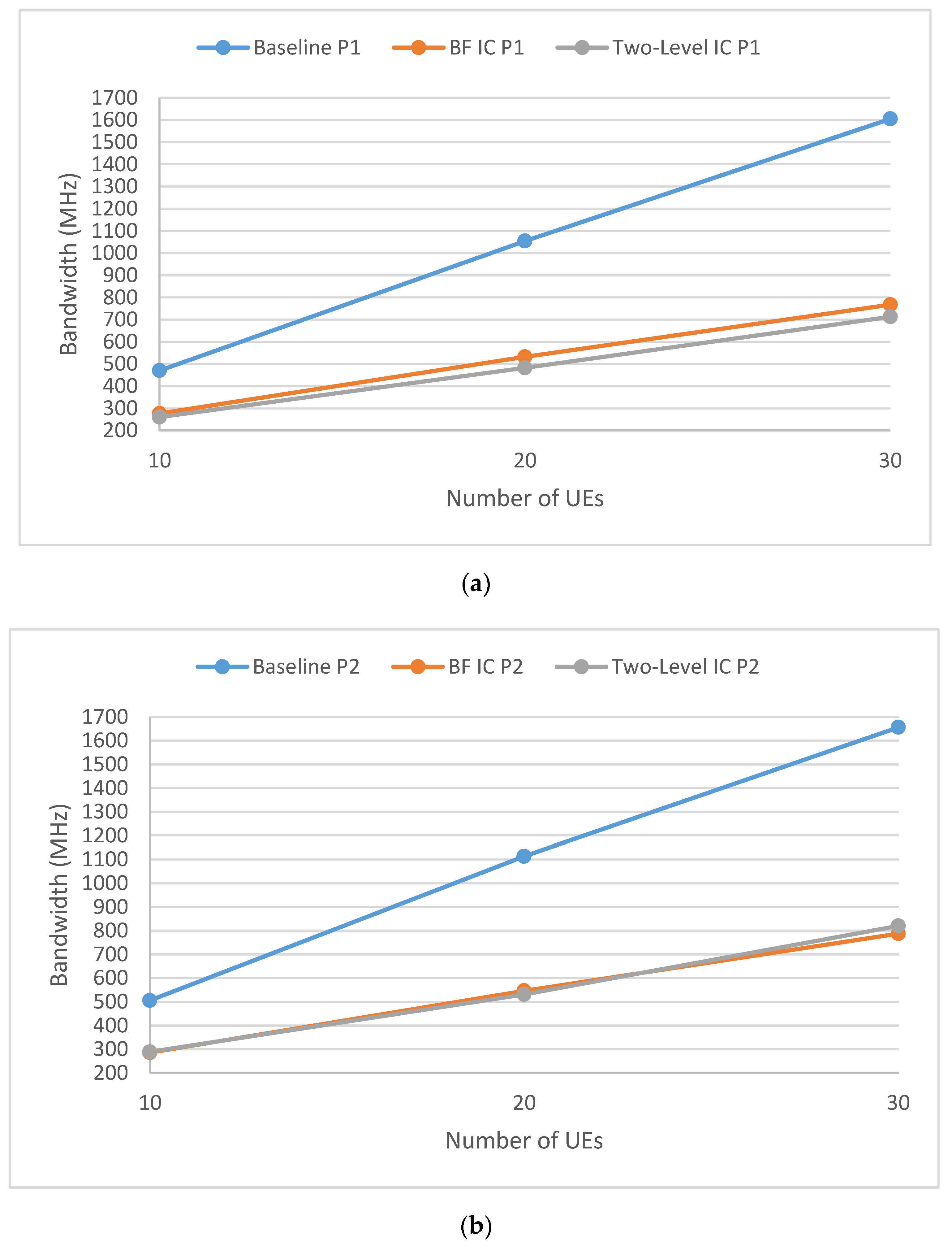
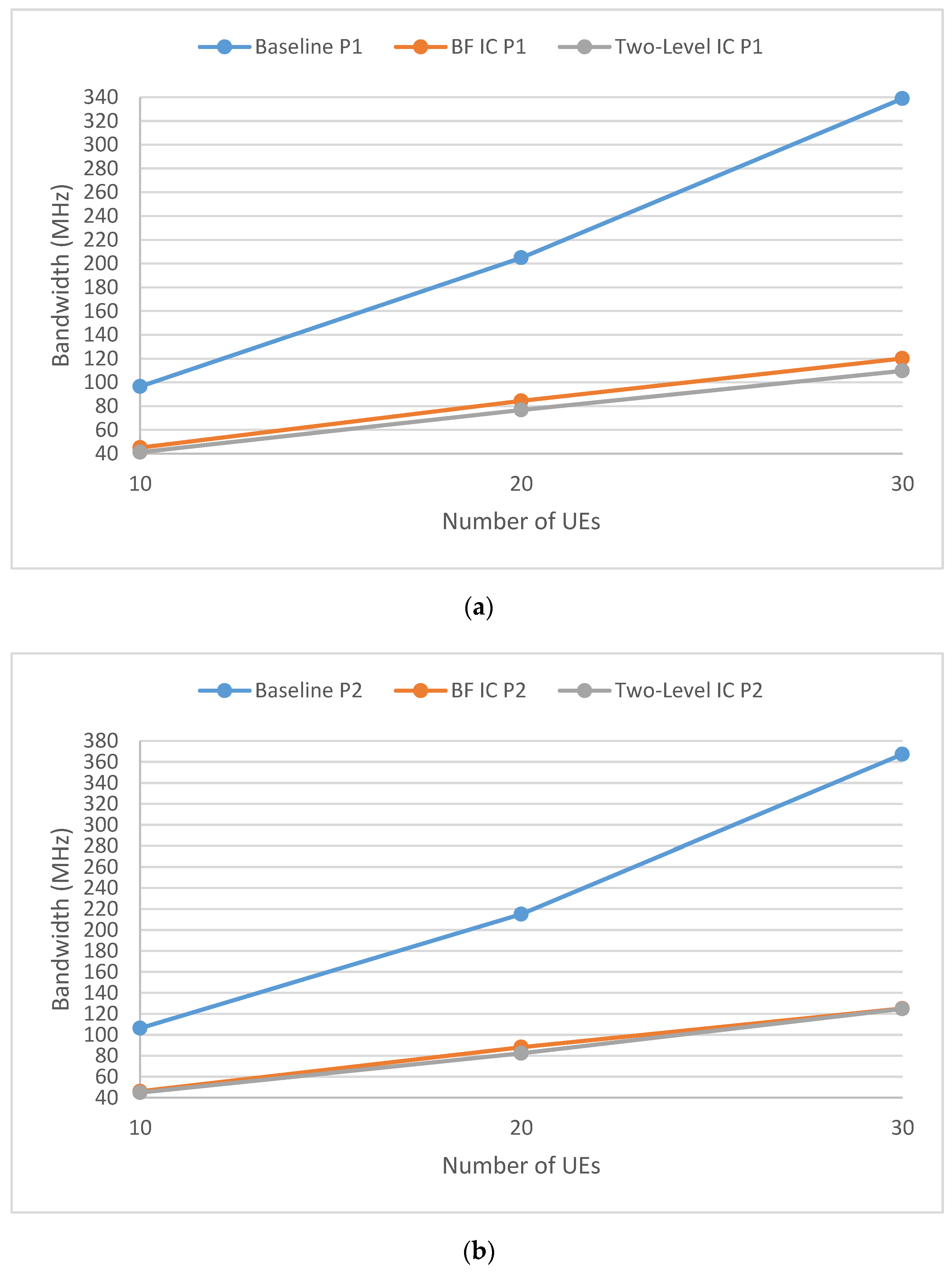
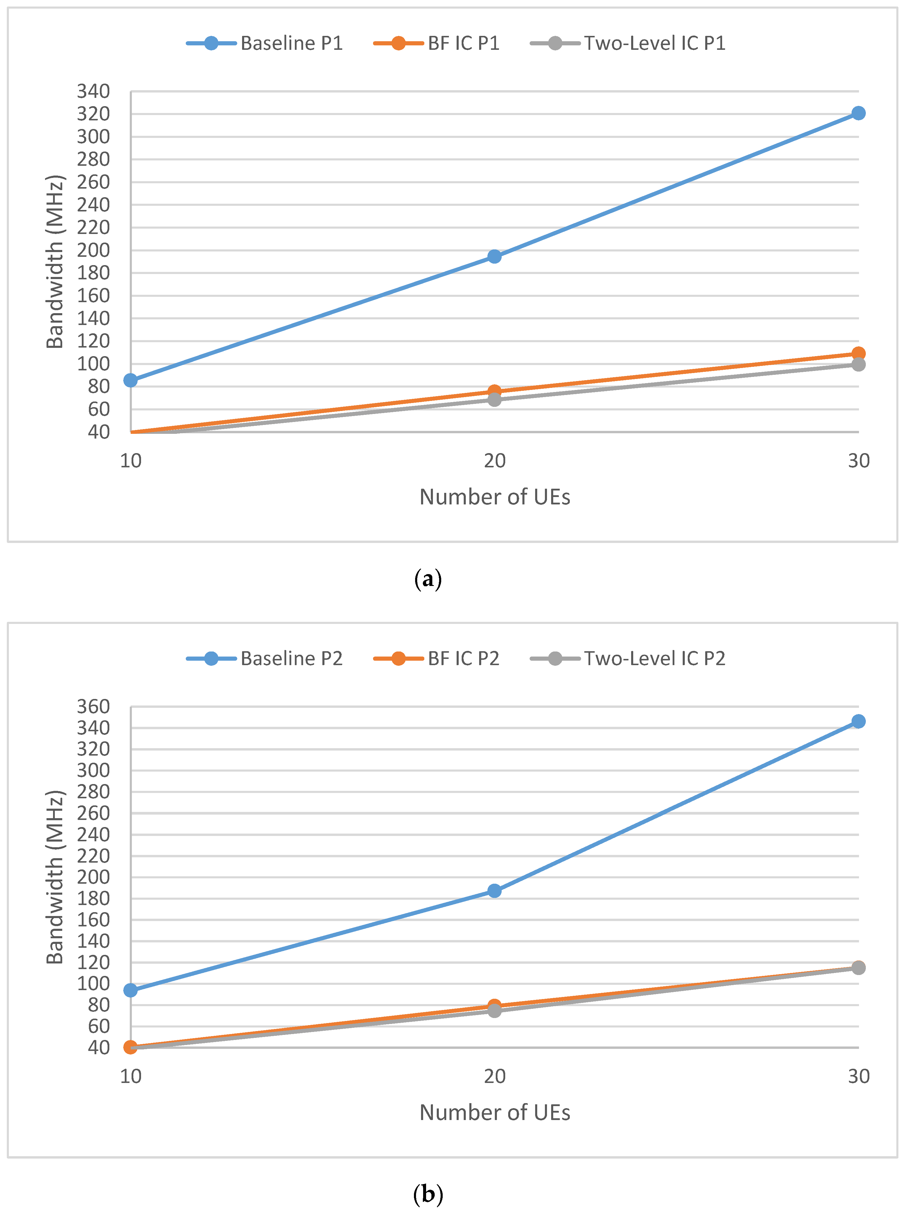
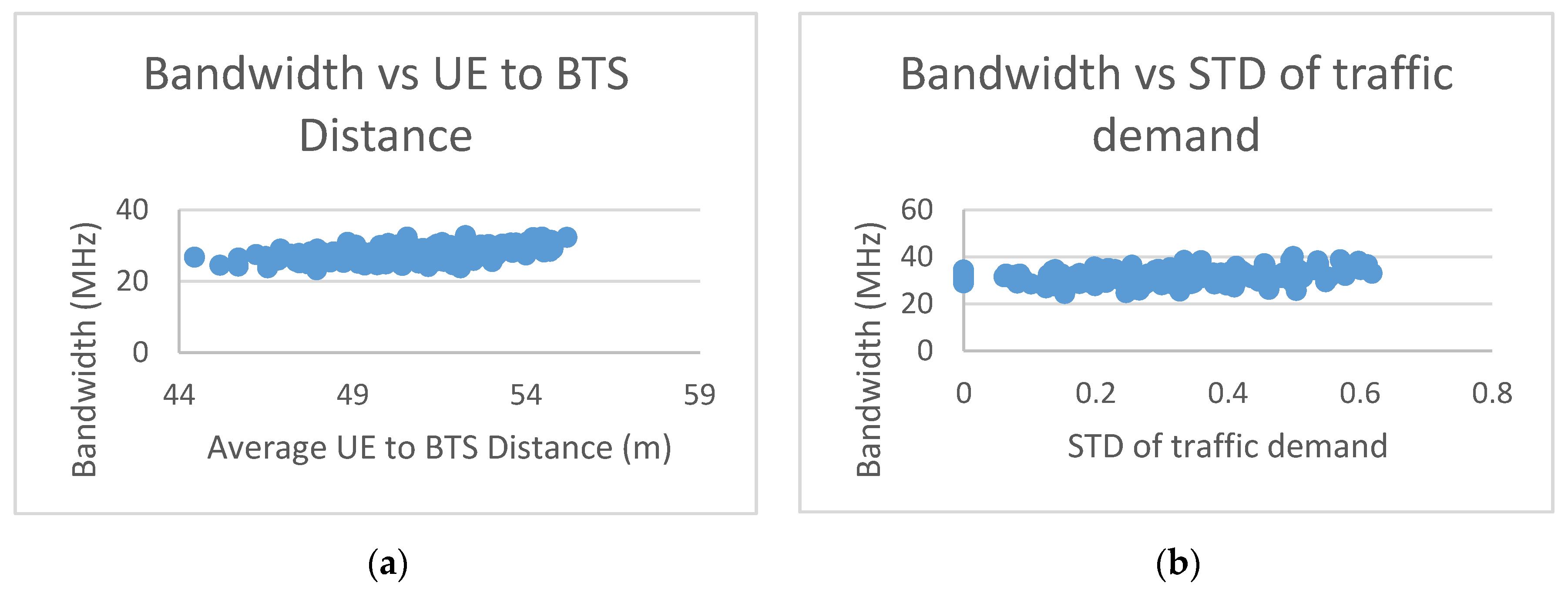
5. Simulation Results

Figure 6 shows the comparison of the bandwidths required for different IC approaches for the virtual reality service (S1) with a 25 M data rate, 20 ms delay budget (90 frames per second (FPS) with 11 ms frame delay and 9 ms transmission delay), and a packet loss rate of 10 3 . This scenario simulated a network with a cell radius of 100 meters (ISD = cell radius × 3 ), 10/20/30 UEs per sector, 4 beams to horizontally cover the sector area, a maximum 3 sectors per cluster, and a maximum of 4 MU-MIMO users per sector. Ten simulations were run with different random seeds, and the results were averaged. The baseline approach is an approach in which no interference coordination is performed. The coordinated beamforming IC approach (BFIC) is a one-level IC approach with intra-cluster interference coordination only. The proposed two-level IC approach, together with the BFIC approach, show improvement in the required bandwidth compared to that of the baseline approach. The two-level IC-P1 approach achieved the minimum required bandwidth, but the two-level IC-P2 approach was worse than the BFIC-P2 approach because of the capacity loss the approach caused.
Figure 7 and Figure 8 are similar to Figure 6. Figure 7 is a scenario for an interactive gaming service (S2), with a 5 M data rate, 100 ms delay budget (40 FPS, 20 ms delay for frame encoding and decoding, and 80 ms transmission delay), and a packet loss rate of 10 3 . Figure 8 shows a scenario for a mix of conversational video service (S3) and non-conversational video service (S4) with 50% loading each. Both services had the same 5 M data rate and a packet loss rate of 10 3 , but different delay budgets (150 ms for S3 with a 130 ms transmission delay, and 300 ms for S4 with a 280 ms transmission delay). Figure 7 and Figure 8 show that the two-level IC-P1 approach achieved the minimum required bandwidth.
Selecting the two-level IC-P1 approach that achieved the minimum required bandwidth, Figure 9 shows the scatter plot of 200 drops with different random seeds. For simplicity, we fixed the cell radius to 100 m, the average number of users per sector at 10, the beams to cover the sector area at 8, and the service as S2 (interactive gaming service). For network design, as explained in Section 3, for each data point (s, u, b, isd, dis, and varT), the maximum required bandwidth is calculated to create the performance model.
Figure 10, Figure 11 and Figure 12 show the network design performance model, simplified by fixing the traffic demand variance varT and the number of beams to 8. The number of UE and the ISD (or the cell radius) were varied with discrete values, and for each data point of (u and isd), 50 drops were run. Figure 13 shows an example of design solution using the performance models in Figure 10, Figure 11 and Figure 12. The SLA requirements include varied UE density (we assume the same UE density among all three scenarios, i.e., N UE per sector for S1, N UE per sector for S2, and N UE per sector for S3 plus S4) and total available bandwidth of 1 GHz. A network design solution was to find an ISD in which the bandwidth was shared among services. In all three scenarios specified in Figure 6, Figure 7 and Figure 8, the UE covered by the sites fulfilled their QoS requirements.
Figure 14 shows the SLA violation rate using a performance model. For simplicity, we fixed the cell radius to 100 m, the average number of users per sector at 10, the beams to cover the sector area at 8, and the service as S2. The first 1000 drops were used to generate the initial performance model. For each new drop, dis and varT were used to search the performance model for a solution and verified whether the solution fulfilled the QoS requirements. If not, a new solution had to be found using Algorithm 4 in Section 3, and the performance model updated. The figure shows that as more drops were run, the rate of successful prediction increased.
The same setup in Figure 14 is in Figure 15, to show the network optimization results for 1000 random drops. On average, a bandwidth saving of 7.5% was achieved, which shows that the bandwidth we used for the initial design is as close to the optimized bandwidth as we can achieve.

6. Complexity Analysis

For the IC approach, additional channel quality indicator (CQI) feedbacks are required for cluster edge UEs. For FWA applications with slow varying channels, the air-link overhead is small. The 5G network uses a dedicated fiber network to connect the baseband unit (BBU) and the remote radio unit (RRU), or between the BTS to exchange intra-cluster scheduling outputs and forbidden relationship tables, both delay and data volume are not of concern.
For computational complexity, multiple SINR values are calculated. On the BBU, the intra-cluster scheduling uses greedy algorithm with complexity of O ( | C | *   U c 2 ) , where | C | is the number of clusters and U c is the number of UE in each cluster, which equals C m a x × U s . C m a x is the maximum cluster size, and U s is UEs per sector. For inter-cluster scheduling, only scheduled cluster-edge UE triggers inter-cluster scheduling, with complexity of O ( N * log ( N ) *   U e ) , where U e is the number of assigned cluster-edge UE, N is the number of cell, and O ( N * log ( N ) ) is the sorting complexity.
For the network design and optimization approach, fewer messages are transferred between the network and the management unit, and they are not in a time-critical situation, delay and data volume are not of concern. For computational complexity, the search algorithm is used for the network design. The algorithm runs offline and with low complexity.

7. Conclusions

In this paper, we introduced a two-level IC approach to improve performance models that map high-level customer-friendly business requirements to low-level network parameters and achieve QoS assurance for delay-sensitive traffic. We also proposed an approach that uses data analytics and machine learning to automate identification of no explicit relationships and dependencies between SLA high-level requirements and low-level network attributes to construct QoS performance models, which are used for network design and optimization.

Author Contributions

J.W. (Jiao Wang), O.B., and J.W. (Jay Weitzen) conceived and designed the study. J.W. (Jiao Wang) performed the simulations. J.W. (Jiao Wang) wrote the paper. J.W. (Jiao Wang), O.B., J.W. (Jay Weitzen), V.S. and M.L. reviewed and edited the manuscript. All authors have read and agreed to the published version of the manuscript.

Funding

This research received no external funding.

Conflicts of Interest

The authors declare no conflict of interest.

References

  1. Li, R.-P.; Zhao, Z.; Sun, Q.; Chih-Lin, I.; Yang, C.; Chen, X.; Zhao, M.; Zhang, H. Deep Reinforcement Learning for Resource Management in Network Slicing. IEEE Access 2018, 6, 74429–74441. [Google Scholar] [CrossRef]
  2. Kapassa, E.; Touloupou, M.; Kyriazis, D. SLAs in 5G: A Complete Framework Facilitating VNF- and NS- Tailored SLAs Management. In Proceedings of the 2018 32nd International Conference on Advanced Information Networking and Applications Workshops (WAINA), Krakow, Poland, 16–18 May 2018; Institute of Electrical and Electronics Engineers (IEEE): Piscataway, NJ, USA; pp. 469–474. [Google Scholar] [CrossRef]
  3. Kwan, R.; Leung, C. A Survey of Scheduling and Interference Mitigation in LTE. J. Electr. Comput. Eng. 2010, 2010, 1–10. [Google Scholar] [CrossRef]
  4. Elayoubi, S.-E.; Ben Haddada, O.; Fourestie, B. Performance evaluation of frequency planning schemes in OFDMA-based networks. IEEE Trans. Wirel. Commun. 2008, 7, 1623–1633. [Google Scholar] [CrossRef]
  5. Garcia-Morales, J.; Femenias, G.; Riera-Palou, F. Higher Order Sectorization in FFR-Aided OFDMA Cellular Networks: Spectral- and Energy-Efficiency. IEEE Access 2019, 7, 11127–11139. [Google Scholar] [CrossRef]
  6. Fan, X.; Chen, S.; Zhang, X.; Xiangning, F.; Si, C.; Xiaodong, Z. An Inter-Cell Interference Coordination Technique Based on Users’ Ratio and Multi-Level Frequency Allocations. In Proceedings of the 2007 International Conference on Wireless Communications, Networking and Mobile Computing (WiCOM ’07), Shanghai, China, 21–25 September 2007; pp. 799–802. [Google Scholar]
  7. Al-Falahy, N.; Alani, O.Y. Network Capacity Optimisation in Millimetre Wave Band Using Fractional Frequency Reuse. IEEE Access 2017, 6, 10924–10932. [Google Scholar] [CrossRef]
  8. Pastor-Perez, J.; Riera-Palou, F.; Femenias, G. Clustering and subband allocation for CoMP-based MIMO-OFDMA networks with soft frequency reuse. In Proceedings of the European Wireless 2017; 23th European Wireless Conference, Dresden, Germany, 17–19 May 2017; pp. 1–8. [Google Scholar]
  9. Attia, E.S.; El-Dolil, S.A.; Abd-Elnaby, M. Performance enhancement based resource allocation scheme using soft frequency reuse for LTE femtocell networks. In Proceedings of the 2017 34th National Radio Science Conference (NRSC), Alexandria, Egypt, 13–16 March 2017; pp. 246–255. [Google Scholar] [CrossRef]
  10. Novlan, T.; Andrews, J.G.; Sohn, I.; Ganti, R.K.; Ghosh, A. Comparison of Fractional Frequency Reuse Approaches in the OFDMA Cellular Downlink. In Proceedings of the 2010 IEEE Global Telecommunications Conference GLOBECOM 2010, Miami, FL, USA, 6–10 December 2010; pp. 1–5. [Google Scholar]
  11. Adejo, A.; Boussakta, S.; Neasham, J. Interference modelling for soft frequency reuse in irregular heterogeneous cellular networks. In Proceedings of the 2017 Ninth International Conference on Ubiquitous and Future Networks (ICUFN), Milan, Italy, 4–7 July 2017; pp. 381–386. [Google Scholar] [CrossRef]
  12. Lindbom, L.; Love, R.; Krishnamurthy, S.; Yao, C.; Miki, N.; Chandrasekhar, V. Enhanced Inter-Cell Interference Coordination for Heterogeneous Networks in Lte-Advanced: A Survey; Cornell University Library: Ithaca, NY, USA, December 2011. [Google Scholar]
  13. Ramli, H.A.M.; Asnawi, A.L.; Isa, F.N.M.; Azman, A.W. A survey of component carrier selection algorithms for carrier aggregation in long term evolution-advanced. In Proceedings of the 2017 IEEE 4th International Conference on Smart Instrumentation, Measurement and Application (ICSIMA); Institute of Electrical and Electronics Engineers (IEEE), Putrajaya, Malaysia, 28–30 November 2017; pp. 1–5. [Google Scholar] [CrossRef]
  14. Deb, S.; Monogioudis, P.; Miernik, J.; Seymour, J.P. Algorithms for Enhanced Inter-Cell Interference Coordination (eICIC) in LTE HetNets. IEEE/ACM Trans. Netw. 2013, 22, 137–150. [Google Scholar] [CrossRef] [Green Version]
  15. Ali, S. An Overview on Interference Management in 3GPP LTE-Advanced Heterogeneous Networks. Int. J. Futur. Gener. Commun. Netw. 2015, 8, 55–68. [Google Scholar] [CrossRef]
  16. Luo, H.; Ni, Q.; Zhang, Y.; Huang, L.-K.; Cosmas, J.; Li, W. CRS interference cancellation algorithm for heterogeneous network. Electron. Lett. 2016, 52, 77–79. [Google Scholar] [CrossRef]
  17. Qu, D.; Zhou, Y.; Tian, L.; Shi, J. User-Centric QoS-Aware Interference Coordination for Ultra Dense Cellular Networks. In Proceedings of the 2016 IEEE Global Communications Conference (GLOBECOM), Washington, DC, USA, 4–8 December 2016; Institute of Electrical and Electronics Engineers (IEEE): Piscataway, NJ, USA; pp. 1–6. [Google Scholar] [CrossRef]
  18. Chang, Y.-J.; Tao, Z.; Zhang, J.; Kuo, C.-C.J. A Graph-Based Approach to Multi-Cell OFDMA Downlink Resource Allocation. In Proceedings of the IEEE GLOBECOM 2008—2008 IEEE Global Telecommunications Conference, New Orleans, LO, USA, 30 November–4 December 2008; pp. 1–6. [Google Scholar]
  19. Chang, R.Y.; Tao, Z.; Zhang, J.; Kuo, C.-C. A Graph Approach to Dynamic Fractional Frequency Reuse (FFR) in Multi-Cell OFDMA Networks. In Proceedings of the 2009 IEEE International Conference on Communications, Dresden, Germany, 14–18 June 2009; pp. 1–6. [Google Scholar]
  20. Zhang, C.; Varma, V.; Lasaulce, S.; Visoz, R. Interference Coordination via Power Domain Channel Estimation. IEEE Trans. Wirel. Commun. 2017, 16, 6779–6794. [Google Scholar] [CrossRef]
  21. Rahman, M. Dynamic Inter-Cell Interference Coordination in Cellular OFDMA Networks. Ph.D. Thesis, Department of System and Computer Engineering, Queens University, Kingston, ON, Canada, July 2011; pp. 1–117. [Google Scholar]
  22. Rahman, M.; Yanikomeroglu, H.; Wong, W. Interference Avoidance with Dynamic Inter-Cell Coordination for Downlink LTE System. In Proceedings of the 2009 IEEE Wireless Communications and Networking Conference, Budapest, Hungary, 5–8 April 2009; pp. 1–6. [Google Scholar]
  23. Wang, J.; Weitzen, J.; Bayat, O.; Sevindik, V.; Li, M. Interference coordination for millimeter wave communications in 5G networks for performance optimization. EURASIP J. Wirel. Commun. Netw. 2019, 2019, 46. [Google Scholar] [CrossRef] [Green Version]
  24. Wong, V.W.; Schober, R.; Ng, D.W.K.; Wang, L.-C. Key Technologies for 5G Wireless Systems; Cambridge University Press: Cambridge, UK, 2017. [Google Scholar]
  25. Hoshino, K.; Mikami, M. Experimental Evaluation of Simple Precoding Technique for Multi-Cell Coordinated MU-MIMO. In Proceedings of the 2017 IEEE 85th Vehicular Technology Conference (VTC Spring), Sydney, Australia, 4–7 June 2017; pp. 1–5. [Google Scholar]
  26. Nguyen, D.H.N.; Le-Ngoc, T. Multiuser Downlink Beamforming in Multicell Wireless Systems: A Game Theoretical Approach. IEEE Trans. Signal Process. 2011, 59, 3326–3338. [Google Scholar] [CrossRef]
  27. Wang, J.; Zhu, H. Beam allocation and performance evaluation in switched-beam based massive MIMO systems. In Proceedings of the 2015 IEEE International Conference on Communications (ICC), London, UK, 8–12 June 2015; pp. 2387–2392. [Google Scholar]
  28. Maruta, K.; Ahn, C.-J. Uplink Interference Suppression by Semi-Blind Adaptive Array with Decision Feedback Channel Estimation on Multicell Massive MIMO Systems. IEEE Trans. Commun. 2018, 66, 6123–6134. [Google Scholar] [CrossRef]
  29. Niu, Y.; Li, Y.; Jin, D.; Su, L.; Vasilakos, A.V. A survey of millimeter wave communications (mmWave) for 5G: Opportunities and challenges. Wirel. Netw. 2015, 21, 2657–2676. [Google Scholar] [CrossRef]
  30. Tung, C.-Y.; Chen, C.-Y.; Wei, H.-Y. Next-Generation Directional mmWave MAC Time-Spatial Resource Allocation. In Proceedings of the 11th EAI International Conference on Heterogeneous Networking for Quality, Reliability, Security and Robustness, Taipei, Taiwan, 19–20 August 2015; pp. 728–742. [Google Scholar]
  31. 3GPP. Technical Specification Group Radio Access Network, Channel model for frequency spectrum above 6 GHz. Available online: https://itectec.com/archive/3gpp-specification-tr-38-900/ (accessed on 6 June 2020).
Figure 1. Gains of a basic antenna.
Futureinternet 12 00099 g001
Figure 2. Power received at the UE [29].
Futureinternet 12 00099 g002
Figure 3. Design process.
Futureinternet 12 00099 g003
Figure 4. Interference Effect.
Futureinternet 12 00099 g004
Figure 5. 2 × 2 MIMO link curve [23].
Futureinternet 12 00099 g005
Figure 6. Different IC approaches for the Virtual Reality service. Sub-figure (a) shows IC-P1 (UIC) approaches and sub-figure (b) shows IC-P2 (GIC) approaches
Futureinternet 12 00099 g006
Figure 7. Different IC approaches for the Interactive Gaming service. Sub-figure (a) shows IC-P1 (UIC) approaches and sub-figure (b) shows IC-P2 (GIC) approaches.
Futureinternet 12 00099 g007
Figure 8. Different IC approaches for the Mixed Video Traffic service. Sub-figure (a) shows IC-P1 (UIC) approaches and sub-figure (b) shows IC-P2 (GIC) approaches.
Futureinternet 12 00099 g008
Figure 9. Bandwidth for multiple drops. The sub-figure (a) shows that as the average distance from the UE to the BTS increases, more bandwidth is required. The sub-figure (b) shows that as the traffic demand varies among the sectors, the variance of the required bandwidth to fulfill the QoS requirement increases
Futureinternet 12 00099 g009
Figure 10. Design performance model of the Virtual Reality service. The sub-figure (a) shows required bandwidth vs. number of UEs per sector at different ISD, the sub-figure (b) shows required bandwidth vs. cell radius at different number of UEs per sector.
Futureinternet 12 00099 g010
Figure 11. Design performance model of the Interactive Gaming service. The sub-figure (a) shows required bandwidth vs. number of UEs per sector at different ISD, the sub-figure (b) shows required bandwidth vs. cell radius at different number of UEs per sector.
Futureinternet 12 00099 g011
Figure 12. Design performance model of the Mixed Traffic service. The sub-figure (a) shows required bandwidth vs. number of UEs per sector at different ISD, the sub-figure (b) shows required bandwidth vs. cell radius at different number of UEs per sector.
Futureinternet 12 00099 g012
Figure 13. Design solution.
Futureinternet 12 00099 g013
Figure 14. SLA violation rate.
Futureinternet 12 00099 g014
Figure 15. Network optimization.
Futureinternet 12 00099 g015
Table 1. Proposed Ic Algorithms.
IC ApproachIntraCluster LevelInterCluster Level
Two level IC - P2IC-P2IC-P2
Two level IC - P1IC-P1IC-P1
Table 2. Forbidden Relationship [23].
UEServingCellConflictUEConflictBMConflictCellConflictUEUtilConflictUEOffUtilConflictUEOnUtil
U E 1 R R U k 1 U E u 1 B e a m m 1 R R U n 1 U t i l u 1 U t i l 1 ,   u 1 O f f U t i l 1 ,   u 1 o n
U E u 2 B e a m m 2 R R U n 2 U t i l u 2 U t i l 1 ,   u 2 O f f U t i l 1 , u 2 o n
U E x R R U k x U E u y B e a m m y R R U n y U t i l u y U t i l x ,   u y O f f U t i l x ,   u y o n

