Article

Adaptive Pre/Post-Compensation of Cascade Filters in Coherent Optical Transponders

School of Electrical Engineering and Computer Science, University of Ottawa, Ottawa, ON K1N 6N5, Canada
*
Author to whom correspondence should be addressed.
Future Internet 2020, 12(2), 21; https://doi.org/10.3390/fi12020021
Submission received: 17 December 2019 / Revised: 21 January 2020 / Accepted: 21 January 2020 / Published: 24 January 2020
(This article belongs to the Section Network Virtualization and Edge/Fog Computing)

Abstract

:
We propose an adaptive joint pre- and post-compensation to correct the filtering effects caused by cascading reconfigurable optical add drop multiplexers (ROADMs). The improvement is achieved without using additional hardware (HW) on the link or within the signal processor in the transponders. Using Monte Carlo simulations, the gradient-descent based method shows an improvement of 0.6 dB and 1.1 dB in the required optical signal-to-noise ratio (R-OSNR) at the threshold pre-decoder bit error rate (BER) of 0.02 versus pre-compensation only in the linear and nonlinear operating region of fiber respectively. We experimentally verified the method with lab measurements in the presence of heavy filtering and optical impairments. We observed a gain up to ~0.4 dB compared to typically used pre-compensation only. Additionally, other tangible system benefits of our method are listed and discussed.

1. Introduction

The deployment of optical switches, such as reconfigurable optical add drop multiplexing (ROADM), was a key milestone in enabling all-optical transmission, as illustrated in Figure 1a, from source to destination in a dense wavelength division multiplexing (DWDM) network. They offer great advantages for service providers such as simplification of network planning and provisioning, reduction in infrastructure cost and lower power consumption (no electrical to optical, and vice-versa, conversion required). Each optical link is split into sections called spans. The latter is characterized by the position of ROADM nodes. The length of fiber per span is in the range of 80 to 160 km depending on the amplification technology used [1]. With flexibility being a requirement in current and future optical networks, ROADMs, which are made using Liquid-Crystal on Silicon (LCOS) [2] or Micro-Electro Mechanical Systems (MEMS) [3] with optical switch fabric, allow control to be done per wavelength both in terms of routing and attenuation. “Broadcast and Select” and “Route and Select” are two main switching architectures based on ROADMs discussed in [4].
ROADMs, acting like filters with limited passband bandwidth, are critical limitations in fixed-grid optical networks [5]. They introduce colored noise to the signal while affecting both the amplitude and the phase of the propagated stream of optical pulses. The system impact of concatenated filtering on 28 Gigabaud (Gbaud), using dual-polarization (DP) 8QAM constellation, was discussed in [6]. Both passband bandwidth-narrowing and ripples are discussed in [7]. As the signal travels from the source to destination on an all-optical link, the aforementioned effects accumulated the signal passes through a series of cascaded ROADMs. This introduces dispersion and spectral clipping which are impairments that lead to performance degradation. Currently deployed ROADMs have fixed-bandwidths of 50 and 100 GHz per wavelength. Deployment of next-generation flexible-bandwidth, enabling flex-grid networks, with a granularity of 6.25 GHz is under-way [8]. Temperature also impacts the frequency response of the Electro-Optics (EO) at the transmitter and receiver which, along with the effects of the ROADMS, causes an overall filtering effect that must be compensated for to minimize SNR penalty. To compensate for the filtering frequency-dependent loss, as illustrated in Figure 1b, the authors of [9,10] discussed applying a pre-compensation at the Tx of a 10G optical transponder. It is assumed that the transfer function (TF) of the channel is measured and available to use. In [11,12], authors studied the impact of pre-compensation, using finite impulse response (FIR) filters at the digital to analog converter (DAC), of the narrowing of bandwidth due to gridless ROADMs. The method assumes the knowledge of the number of ROADMs in the link and the center frequency offset. In [13], the authors introduced new hardware (HW) block, a trellis decoder, at the end of the Rx processing chain. The solution requires extra processing and cause higher power consumption. In [14], the authors suggested using external optical wave-shapers at the edge of the DWDM link. The concept is similar to the Dispersion Slope Compensation module, described in [15], that deals with compensating for chromatic dispersion per span along the link. However, besides the cost, maintenance and power consumption of new modules in link, the shapers have to be programmed for initial deployment. which makes network planning more burden but will lack continuous track of changes in transferring frequency response due to temperature or drift in center frequency when MEMS’ mirrors ages. In [16], time-domain hybrid modulation is used to reduce the gap between the R-OSNR of regular M-QAM constellations, therefore provides flexible line-rate transmission. The authors presented super-symbols as a combination of 8QAM and 16QAM and showed that, as expected, hybrid modulations perform in between the two even when propagating through heavily filtered channels.
In this paper, we present a new software-based method that uses existing HW blocks in a typical coherent Rx, to reduce the Required-OSNR (ROSNR) of an optical link in the presence of ROADMs filtering. The source of filtering in optical links is detailed in Section 2. The models used for the filtering and architecture of typical dual-polarization coherent Rx are illustrated in Section 3. In Section 4, we will show the mathematical derivation of the proposed gradient-descent based method. The channel model, simulation environments and results are described in Section 5. In Section 6, the method is validated through a lab experiment. In Section 7, we discuss the feedback channel, present system advantages of our method and compare simulation to a lab experiment.

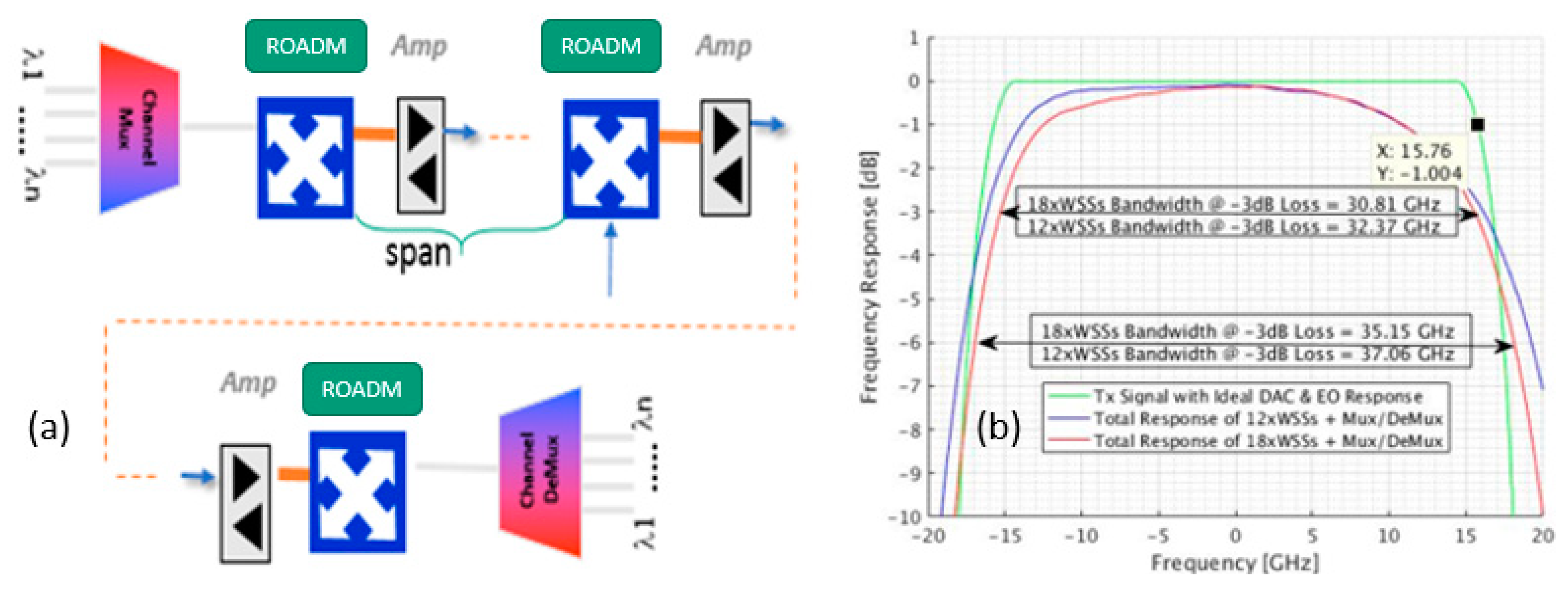
2. Sources of Filtering in Optical Links

With fixed-grid switching elements, wavelength selective switches (WSSs) and channel mux/demux (CMD), being built with different technologies, as well with diverse manufacturing variations and a large number of suppliers [17]. Therefore, the predictability of the frequency response and center frequency shift of the concatenation of all the filtering effects is a challenge. In [17], the distribution of center frequency offset varies from the range of (−1, +1) to (−4, +4) GHz. As presented in [18], each WSS port can be modeled as super-Gaussian and is specified by two parameters: (1) 3 dB frequency width ( σ s g ) and (2) order ( n ):
S s g ( f ) = 1 σ s g 2 π exp [ ( f 2 2 σ s g 2 ) n ] .
While in [19], the characterization of 96 CMD instances built with arrayed-waveguide gratings (AWG) technology, showed a variation of +/−5 GHz around channel nominal frequency. As well, the insertion loss per port varies and alters the shape of the propagated waveform. For our simulations and laboratory experiments, we got the frequency response of the aggregation of 18 commercial 50 GHz fixed-grid WSSs and one set of worst-case Multiplexer (Mux)/Demultiplexer (Demux) of a 50 GHz fixed grid CMD. The responses, showed in Figure 1b, include some ripples in the passband. The phase response was ignored for two reasons: one is that the concatenation of filters causes a reduction in the phase ripple variance (based on our observation and, that can be explained with the law of large numbers), second is that the adaptive filter at the receiver can correct for phase disturbance with no penalty.

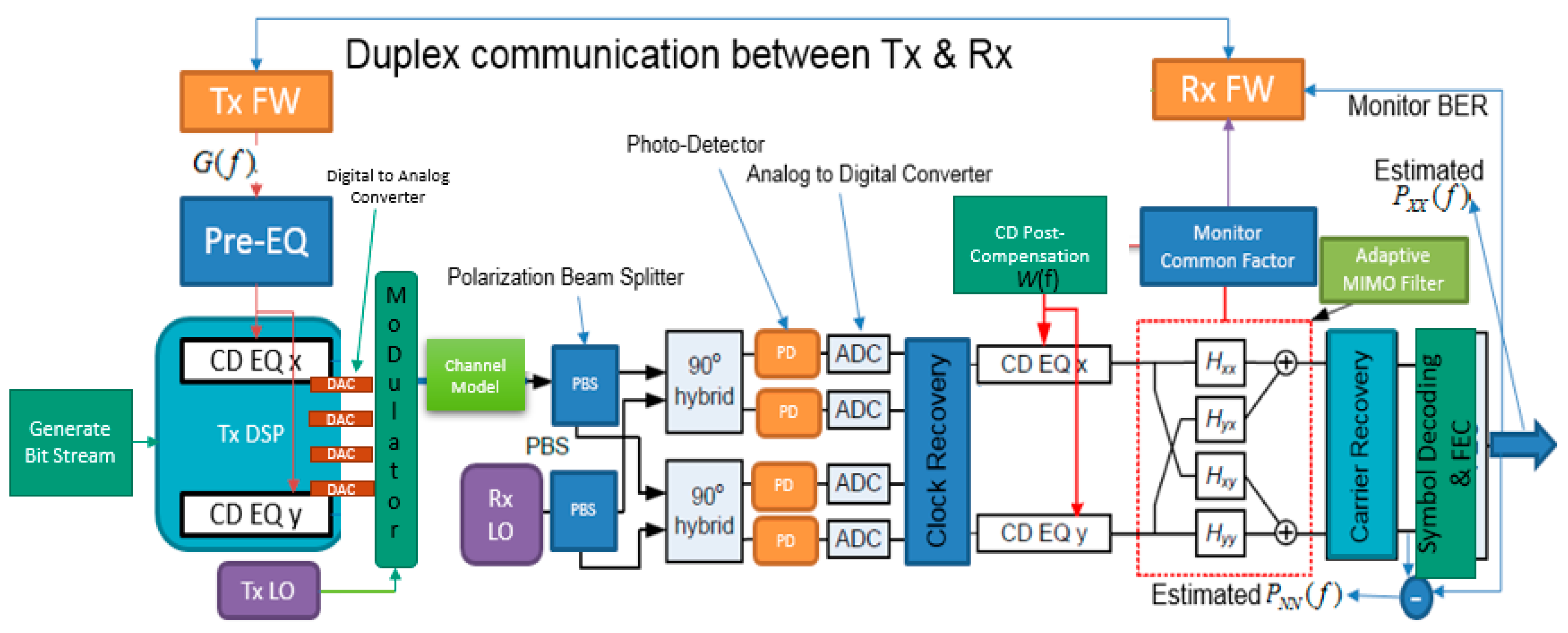
3. Adaptive Filtering in Coherent Receivers

In Figure 2, we illustrate the typical blocks in a coherent transponder. In the Tx, data streams are encoded then filtered with a static filter (CD EQ_x/y). The static filter is used for pulse shaping to reduce intersymbol interference and for dispersion pre-compensation. It is shown in [20] that splitting the dispersion compensation between Tx and Rx improves performance in the presence of nonlinearity, such as in long-haul propagation. Tx/Rx Firmware (FW) blocks, shown in Figure 2, represent the software-based routines used to provision/control the digital (such as update filters coefficients and provide telemetry information to the higher application in the networks) and EO portions of a transponder.
A dual-polarization optical signal is split and mixed with the output of a local oscillator at the Rx to generate four branches (X/Y polarizations, each has in-phase and quadrature field). The data is digitized using an analog-to-digital converter (ADC) then goes to digital signal processing blocks. At the receiver, static filters (denoted as CD EQ x and CD EQ y in Figure 2) are used as matching the Tx filters to maximize SNR and for dispersion post-compensation. Root raised cosine (RRC) filters are used to form a raised cosine (RC), before adaptive filtering, to minimize inter-symbol interference (ISI). It is typical that the bulk part of dispersion is compensated prior to symbols reaching the butterfly MIMO equalizer. The latter is the core of the Rx and it is adaptive, where Constant Modulus Algorithm (CMA) and Least Mean Square (LMS) are examples of the adaptive method used [21], to decouple the two polarizations and compensate for linear time-variant channel impairments such as Polarization Rotation, Polarization Mode Dispersion (PMD) and Polarization Dependent Loss (PDL).
Impairments such as residual dispersion, filters passband ripples, and edges roll-off are quasi-static (i.e., varies very slowly with fiber and components aging/temperature)—they can be estimated using the common factor of the four Multi-Input Multi-Output (MIMO) filters. In [22], the use of a common response was introduced to remove some of the residual dispersion from the adaptive filter and transfer them to the static filter to increase the Rx tolerance of PMD. In our case, instead of using the phase of the common response, we will use the magnitude to help mitigate the filtering effects. Frequency and phase offsets, between Tx and Rx laser oscillators, are tracked by carrier recovery block using methods such as Viterbi-Viterbi [23]. Symbol decoding, or de-mapping, and forward error correction (FEC) work together to extract and correct the sent stream of bits from the received symbols. As described in [24], they both can be based on soft-decision, such likelihood metric, or hard-decision. The 2 × 2 MIMO equalizer matrix can be represented as:
H ( f ) = ( H x x ( f ) H x y ( f ) H y x ( f ) H y y ( f ) ) ,
With the common response that is shown in [22]:
H c ( f ) = H x x ( f ) H y y ( f ) H x y ( f ) H y x ( f ) .
In practice, the common response is estimated using time averages. The accuracy of the averaged response is improved as we increase the duration of the time average, especially in the presence of strong amplified spontaneous emission (ASE) in the link. With no impairments, such as frequency selective loss and dispersion, the symbol arrives at the Rx within its “dedicated” interval. Otherwise, we see the ISI effect where the transition of the symbols scatters to the neighbor intervals. Digital compensation is basically applying different weights and delays, i.e., filtering, to undo the expansion caused by neighboring symbols over the symbol of interest. The size of the filters required depends on the characteristic of the channels. In the frequency domain, the compensation is mainly pre-emphasizing high-frequency components of the data stream. Beside ROADMs, data converters (ADC/DAC), driver and optical modulator can have some roll-off at high frequencies [25]. In [26], it is mentioned that the DAC frequency response at 80% of Nyquist sampling frequency, from the output amplitude is attenuated by 2.42 dB. We demonstrate how the amplitude of the common response Hc(f), presented in Equation (3), is capturing the quasi-static frequency-dependent ripple and loss from output of Tx DAC to the input of Rx ADC. In a lab experiment, with a commercial card, we captured the four vectors of FIR filters taps (Hxx/Hyx/Hxy/Hyy) 50 times, with five ms period, as shown in Figure 3a. The latter illustrates how consistent is the common response in estimating the static frequency response, both phase (as demonstrated in [22]) and amplitude.
Since the frequency responses of the filters have intense drooping at high-frequencies, and the center frequency is at an offset (which emphasizes one side of the spectrum), we can see more peaking of about 5 dB on the high positive frequencies compared to negative ones. In the mid-range of the frequency response, the ripples are compensating for both the ripples in channels and the residual ripples from Tx EO/Rx EO/DAC/ADC calibrations. The average of the retrieved common responses of three different scenarios, displayed in Figure 3b, are used in the optimization process. The approximation of the shift in the center frequency, from the International Communication Union (ITU) center frequency, is embedded in the estimated frequency response; it is visualized when comparing blue and red curves below. The x-axis is the index of the frequency bins used in the operation, they are mapped to −20 to +20 GHz, i.e., +/−sampling frequency/2 (referred to as Fs/2). Since PDL accumulates in a link mainly due to birefringent elements, such as mechanical stress or variability in the manufacturing process as described in [27], and Wavelength Selective Switches (WSS), as detailed in [28]; therefore, we modeled the maximum PDL in association with filtering.

4. Derivation of Proposed Method

Without power constraint, pre-shaping (or pre-compensating for frequency loss) data only at the Tx would give the best performance since most of the noise, mainly from ASE in fiber link, has not yet been introduced. However, in practice, transceivers operate with total power constraint over the signal spectrum ( B ).
P c h = f = F r e q   S t a r t F r e q   S t o p 10 F F T B i n ( f ) 10 B .
We propose a new method to do the joint compensation (of both vectors G and W shown in Figure 2) that takes into consideration the noise and power limitation at the output of the Tx. We propose a gradient-descent approach that compensates for the cascade of ROADM filter effects encountered by an optical signal when routed from the Tx to associated Rx. It is required to transfer the estimated pre-emphasis spectrum to the Rx where all computations can be executed. There are three ways at least to enable the communication: (1) using service channel, usually low data rate, that serves all modems in a node, (2) part of the data overhead in the communicated signal in duplex manner and (3) information of all modems in a software-defined networks ecosystem and a management protocol, such as Network Configuration Protocol (NETCONF), can be used to exchange the coefficients required at the Tx.
In this paper, we only look at compensating for the magnitude response. We ignored the phase response because we could show that the adaptive filtering, LMS in our case, is able to correct for phase distortion with no penalty. First, we consider the Wiener solution, [29,30,31], in an adaptive equalization context. Once a steady-state is reached, the MIMO adaptive filter at the coherent Rx converges to a near-Wiener solution (as we are dealing with time-varying channel model). Since both polarizations go through the same filtering effect, we can use one of them in our procedure. We are assuming that the received symbols are pre-shaped with G and impacted by channel response (estimated as H c 1 ). In the frequency domain, the input of the adaptive filter of the Rx is:
Y ( f ) = X ( f ) G ( f ) H c 1 ( f ) + N ( f ) ,
where X is frequency-domain (Fourier transform) representation of the decoded symbols (at the input of the Forward Error Correction (FEC)), representing the estimate of transmitted symbols, and its power spectrum density is defined as Pxx. Y is the Fourier transform of the received symbols at the input of the receiver filters. Hc is the estimate of the static portion of channel frequency response. G is the frequency domain of pre-compensation coefficients applied at the Tx and N is the Fourier transform of the total noise, with power spectrum density PNN, estimated from the error used in the adaptive filters’ coefficients update. When the cost function is specified the minimum square error, then Wiener equalization/filtering is the optimal solution [30]. Based on the familiar orthogonality principle [31], where the optimal filter is estimated based on the error being orthogonal to the data being used. We define S X Y and S Y Y as, respectively, the cross-correlation between the input and the output and the auto-correlation of the input.
W ( f ) = S X Y S Y Y
The denominator, power spectrum of Y ( f ) , is derived from Equation (5) as follows:
S Y Y = E [ Y ( f ) Y ( f ) ] = P X X ( f ) | G ( f ) ( H c 1 ( f ) ) | 2 + P N N ( f ) .
The numerator, cross-power spectrum of Y ( f ) and X ( f ) , is derived from Equation (5) as follows:
S X Y = E [ X ( f ) Y ( f ) ] = P X X ( f ) G ( f ) ( H c 1 ( f ) ) .
We can show that the Wiener equalizer in the frequency domain, W, is given by the following equation, with * conjugate operators:
W ( f ) = P X X ( f ) G ( f ) ( H c 1 ( f ) ) P X X ( f ) | G ( f ) ( H c 1 ( f ) ) | 2 + P N N ( f ) .
The goal is, through cooperative design, to minimize the mean square error (MSE) between the transmitted symbols and their estimates. As our spectrum is split into M (=256 in our case) frequency bins; therefore, we have to jointly estimate both G ( f i ) and W ( f i ) for i = 1 M . It is worth noting that if noise at the channel output is negligible, P N N ( f ) is approximated to zero and zero-forcing equalization can be used as near optimum. We define F as:
F = i = 1 M E { ( W ( f i ) Y ( f i ) X ( f i ) ) 2 } .
Rearranging (10), we get:
F = i = 1 M N ( f i ) | H c 1 ( f i )   G ( f i ) | 2 + N ( f i ) .
Then gradient descent approached can be used, with µ defined as the step size. We picked a small value equal to 0.1 considering the slow dynamic of moving elements (such as the variability of total TF of cascaded WSSs over temperature):
G ( f i ) = G ( f i ) + µ F G ( f i ) .
With the correction factor derived as:
F G ( f i ) = 2 | H c 1 ( f i ) | 2 G ( f i )   N ( f i ) ( | H c 1 ( f i )   G ( f i ) | 2 + N ( f i ) ) 2 .
Normalization is required due to the total optical power constraint at the output of the Tx:
G _ n o r m ( f i ) = G ( f i ) P c h .
Finally, since both the estimated signal and noise profile are available at the output of the Rx, we can jointly derive W ( f i ) based on Equation (9) by replacing G with G _ n o r m .

5. Simulation Setup and Results

5.1. Simulation Environment

Figure 2 is an overview of the block diagram of the elements used in the simulation to evaluate the methods proposed. The modulation format of choice was 16QAM with the signal baud-rate equal to 35 GBaud and the RRC roll-off factor set to 0.14. The total bandwidth of the signal is 39.9 GHz. The LMS-based adaptive filters each have 17 taps in the time domain. The EO models were ideal, i.e., brick-wall shape with flat passband in spectrum till Fs/2. In these simulations, both the frequency and phase of Tx and Rx local oscillators (LO) are equal; therefore, carrier recovery is not active. As well, EO models are set to the ideal flat spectrum. Symbol identification was a simple search for minimum Euclidian distant per polarization for each received time-domain symbol from carrier recovery. Unlike the work done in [11,12], we are not covering power loss, so we normalized the root-mean square (RMS) of the signal is in simulation. While in the lab experiments, the erbium-doped fiber amplifier (EDFA) was set in power-mode to keep received power the same. The latter was chosen so RMS of the received signal is in the optimum spot for the analog-to-digital converter (ADC). Three set of filters were simulated with each combined with the TF of the common multiplexer/demultiplexer. The 3 dB bandwidth of the final concatenation for 12 and 18 WSSs, Figure 1b, are 30.8 GHz and 32.37 GHz respectively. The model of PDL, used in this correspondence, is the following:
H p d l = [ cos ( θ ) sin ( θ ) sin ( θ ) cos ( θ ) ]   [ 1 0 0 k ]   [ cos ( β ) sin ( β ) sin ( β ) cos ( β ) ]
where 0 < k < 1. The attenuation in dB is:
P D L d B = 20 l o g 10 ( k ) .
Since θ and β are randomly varying, the two polarizations (X and Y) are mixed in a time-varying manner. It is up to the adaptive filter at the Rx to correct and track for the time-varying crosstalk effects. The overall fiber model, Figure 4, used is a concatenation of a channel Mux, filtering effect (N times), noise source to mimic the ASE coming from the Erbium-doped fiber amplifier (EDFA) in each span, bulk PDL element, and CMD Demux. The EDFAs are typically used in every span to compensate for the loss of fiber and insertion loss of optical components.
The instantaneous PDL, resulting from contributions of many random birefringences in fibers and optical components along the link, can be chosen from a Maxwell-distribution. Therefore, in deployed fibers, the total PDL observed by the Rx is statistical and varies with time. In both our simulation and experiment, we fixed the value of PDL and applied continuous random rotations before and after, as in Equation (12). The value of θ and β was set to rotate at a speed of 800 Hz (maximum rotation measured in buried fibers [32]). The BER was averaged out over the length of the frame required by the FEC. Typically, as used in our simulations, the FEC is preceded with an interleaver to scramble the errors in a burst of symbols (avoiding congested errors that will cause traffic hits). We emulated a turbo FEC of size 256 × 256 bits and interleaver of the buffering depth of 24 bits, addition to 4 bits per symbol and 25 pico-seconds per sample, we are simulating 2643 combinations of θ and β.
The clocking of both DAC and ADC is driven by Phase Locked Loop (PLL). At both the Tx and Rx, the dominant sources of jitter in PLLs are the VCO (voltage controller oscillator), reference clocks, frequency dividers and CP (charge pump). With respect to the VCO, it is subject to jitter accumulation which manifests itself as high phase noise at low-frequency offsets with respect to the carrier frequency. Therefore, a jitter profile added to simulation is a must to get realistic results. A white Gaussian timing jitter profile, with a standard deviation of 0.8 pico-seconds, is assumed combined at the DAC and ADC.

5.2. Results in Fiber Linear Regime

We start by studying the effect of filtering and PDL on the system performance without any kind of optimization, i.e., the adaptive MIMO filters at the Rx is compensating for all the impairments. In Figure 5, all data are with a frequency offset of the filter models that are set to 0 GHz, therefore, they are modeled as presented in Figure 1b. The ROSNR was measured by sweeping BER versus five OSNR values, then performing an interpolation.
We notice that the ROSNR penalty, at 2% (=0.02 or 2 × 10⁻² BER, versus PDL can be fit to a quadratic function. The penalty of PDL equal to 7.5 dB is aligned with the results reported [33]. As well, as expected, the penalty when aggregating PDL and filtering impairments is bigger than adding the penalty of each impairment tested individually. The reason for the ROSNR penalty is that both impairments are inducing colored noise that affects amplitude. Since the receiver is equalizing the signal so it brings back the two polarizations to be equal and the spectrum to be flat, then the noise will be boosted as well. Therefore, both PDL and filtering can’t be corrected, as PMD and chromatic dispersion, but can only be compensated.
As well, when the adaptive filter is compensating for more than one impairment, the taps continuously trying to converge to the solution with the minimum mean square error, however, they are prone to misadjustment and hence higher penalty when aggregated. The penalty of 12xWSSs without PDL is ~1.05 dB, while when added to PDL, it is ~1.2 dB. The higher the noise in the link, i.e., low OSNR, the more advantageous to amplify the signal right at the transmitter since symbols are not corrupted with errors yet. However, to keep the power constant, the peaking of high-frequency components comes at the price of de-emphasizing the low-frequency bins. Hence the trade-off. However, real transmitters have implementation noise due to quantization (limited bits resolution of both filter taps and QAM symbols), their static filters taps are near clipping and effective number of bits (ENOB) at the DAC is a function of frequency; therefore, emphasizing frequency bins at the transmitter might be deteriorating rather than helpful. For “Tx Equalization” only, there are two means to implement it. One is zero-forcing which uses the common response of the Rx and apply it with pulse-shaping and required pre-compensation at the static filter. Energy in frequency bins is always normalized to keep output power constant.
H T x ( f ) = H R R C ( f ) H C M D 1 ( f ) | H c ( f ) | .
The second technique, used to compare our method against, is MMSE-based as it takes SNR into consideration. In Equation (17), T F m e a s u r e d ( f ) is set equal to inverse of the TF of the total filtering effects. While T F t a r g e t ( f ) is simply the flat response aimed at the input of the Rx. S N R f a c t o r is the noise adjustment term which can be scanned to get optimal BER.
P e a k i n g T x ( f ) = T F t a r g e t ( f ) T F m e a s u r e d ( f ) + S N R f a c t o r .
At 2% BER, we notice that when method converges (after around 40 iterations on average with the loop running ones every 10 seconds), most of the compensation (~70%) of the steep roll-off of the cascaded filters (as shown in Figure 1b) occurs at the Tx. While the remaining 30% is applied to the static filter of the receiver. At lower BER, i.e., higher link OSNR, the ratios will change. The reason is that it might not be as beneficial to pre-emphasis data since the noise-induced is small. Such observations are explained by Wiener’s optimal solution in presence of pre/post-compensation, Equation (6), where the noise components are showed up in the denominator. As the noise gets larger, the post-compensation gets smaller and vice-versa.
With 18xWSSs and PDL of 7.5 dB, splitting the compensation of the steep loss at high frequencies between the Tx and Rx, with minimum mean-square-error at receiver as criteria, reduced the ROSNR by 0.6 dB compared to 0.3 dB when performing pre-compensation only (as shown in Figure 6). The penalty versus center frequency offset, due to the mismatch between the carrier frequency and center of concatenated filters, is highly dependent on the symmetry of the frequency response of the channel, EOs and frequency response of data converters. The reason is that all the frequency responses will be multiplied by the signal, with noise added at different stages of the propagation chain, prior to being processed by the receiver. As expected, and similar results to data presented in [34], the penalty versus frequency offset has minimal around 0 GHz and gets larger on both positive and negative edges. As in other published results [11], compensating for the phase information of the filtering effects did not make a difference in our data. It was noticed that the phase distortion is dealt with properly in the adaptive filters at the receiver.

5.3. Results in Fiber Nonlinear Regime

In our Monte-Carlo simulations, we use the typical standard single mode fiber (SSMF) parameters, listed in Table 1. Nine WDM, with spacing of 50 GHz, channels are co-propagated with the middle channel chosen as probe to study the impact. With SSMF modelled as part of the ROADM in Figure 4, the launch power swept is from −1 dBm to +1 dBm by 0.5 dBm step.
With x is time-domain signal measured at DAC output and M the number of samples, PAPR is defined as:
P A P R = max | x m ( n ) | 2 E { | x m ( n ) | 2 } , m = 1 , , M .
It is observed that by optimizing the split of amplitude compensation between the Tx and Rx, the peak to average power ratio (PAPR) was reduced, at the Tx, by 0.78 dB in the case of 18xWSSs and 0.57 dB in the case of 12xWSSs compared to the PAPR when full pre-compensation of channel response is used. Our results show a reduction of 0.8 dB and 1.1 dB in R-OSNR, versus pre-compensation only, which is shown for 12xWSSs and 18xWSSs cases respectively. The gain is a combination of improvement in linear and nonlinear performance. Therefore, the reduction of PAPR is acting as fiber nonlinearity mitigation. Since nonlinear effects in long-haul fiber propagation are proportional to the instantaneous power of the transmitted signal, as shown in [35], therefore high PAPR would decrease system performance. Lessening the PAPR, as discussed thoroughly in literature especially in the context of OFDM and multi-carrier transmissions [36,37,38], is one of the main methods to mitigate the nonlinear effects in long-haul propagations in fiber. From the nonlinear perspective, our results are consistent with [39], where authors showed that a reduction of 1 dB, from 7 to 6 dB, improved Q-factor by more 0.8 dB in 1040 Km propagation for coherent-optical orthogonal-frequency division multiplexing (CO-OFDM) simulation.

6. Experimental Setup and Results

A set of experiments was conducted to get the quantitative benefits in real-world settings using the setup in Figure 7. We tested channel propagation with PDL emulator, PMD and Polarization Controller. PC1 and PC2 used to scramble the two polarizations, emulating state-of-polarization (SOP) variation, at a rotation rate of 800 Hz. Noise was added, with 50/50% combiner, by controlling the variable optical attenuator (VOA) setting at the egress of the amplifier spontaneous emission (ASE) source.
The LCoS-based 1 GHz resolution waveshaper was used to mimic two different optical links, as shown in Figure 1b, with the frequency responses of both CMD Mux and Demux subtracted. Instead, we used real AWG-based CMD at both sides, which helped to filter the noise before the signal is received. PMD emulator was programmed to introduce 30 ps. Variation in PMD, along with state of polarization, can be corrected at the receiver with no penalty. Its introduction here for completeness to mimic both random birefringence in fiber links and not directly related to WSSs. As well, based on results shown in [40], using a high-resolution measurement technique, a MEMS-based WSS has an upper-bound PMD value of 30 femto-second per port. The commercial card was set in loopback through the experimental work, therefore once acquired, the laser was centered at ITU wavelength of 1546.92 nm (equivalent to 193,800 GHz), and only dithering within a frequency range of 200 MHz since it is locked to itself. An optical spectrum analyzer with a fine resolution of 300 MHz, using 90/10% splitter, was used in the measurement of the transmitted spectrum with and without pulse shaping, and filtering effects programmed at the waveshaper. The sweeping of OSNR was done with varying the setting of VOA. The setup was characterized according to IEC 61280-2-9 standard. To minimize error, all reported OSNR values are the average of 10 consecutive measurements, with accuracy within 0.1 dB.
In Figure 8, using two commercial cards, the advantage of using the proposed method is presented for different jitter profile and various Tx EO responses. A maximum gain of 0.38 dB in Required-OSNR is measured when the total jitter root-mean-square (RMS) is 1 picosecond (ps), equivalent to 3.5% of unit-interval (UI). With DAC PLL is jittery and the EO response has steep roll-off at high-frequencies, equal 6 dB loss at 15 GHz, balancing the compensation of the channel filtering has a high-gain compared to performing only pre-compensation. Especially that the clipping effects, at the Tx filter, introduce a bias noise that impacts the SNR. The clipping is caused by the necessity to peak more than the maximum allowed magnitude per frequency bin. For lower jitter (i.e., better clocking quality), as we will discuss in detail in Section 7.1.3 below, and relaxed Tx EO response of 3 dB loss at 15 GHz, the gain is less obvious. With the same card, i.e., same EO responses to ease comparison, when jitter RMS is 1.8% (0.5 ps) and 2.7% (0.75 ps) of UI, the gain is up to ~0.26 and ~0.15 dB, respectively.

7. Discussions of Results and Research Findings

7.1. Comparison of Contribution to Other Published Methods

We proposed a new software-based method that uses typical/existing HW blocks in coherent optical transponders and software-based feedback loop to continuously optimize both Tx and Rx FIR filters based on estimated channel response and signal-to-noise ratio (SNR) at the Rx. Comparing to published methods, we are highlighting the following key differentiators:

7.1.1. No Extra Hardware and No Required Knowledge of Light-Path

Our method does not imply any extra power consumption, compared to other methods using power-consuming time domain FIR or trellis decoders. In [9,11], there is no mention of how the T F m e a s u r e d ( f ) (as in Equation (15)) is obtained. Besides, when using the number of ROADMs to estimate the order/bandwidth (applied to Equation (1)), the variability in both ROADMs and CMDs response can be big and hence higher margin for divergence from optimality. With the introduction of colorless CMD, new ROADM-based architectures described as Colorless-Directionless-Contentionless (CDC) Mux/Demux are heavily deployed in nowadays’ mesh networks [41]. The latter may have more than hundreds of light-paths [42] and deploy multi-degrees ROADMs, up to 8 degrees using WSSs with 43 ports as presented in [43,44], per site where any tunable Tx can be connected to any colorless CMD port. Having said that, pre-setting the correct pre-equalization TF or programming FIR filter taps properly takes an enormous effort and it’s prone to mistakes. Since only the Rx can estimate the channel response, any automated method requires a feedback channel. In [45], the authors introduced FIR filters post-ADC in order to adaptively correct for bandwidth narrowing due to electronics and optical chains. Such filters will increase the design complexity and power consumption.

7.1.2. Requirement for a Communication Channel Between Tx and Rx

With software-defined networks being designed, providers are moving to automated, zero-touch and zero-provisioning optical networks. Carrier-grade requirements are focused on features such as automatic rerouting and adaption of line rate based on available OSNR on the link [16]. Having said that, a backchannel between Tx and Rx will be a must in current and next-generation intelligent transponders. The feedback communication can be done using an optical service channel, if available in the network. Otherwise, since the vast majority of optical fiber deployments are duplex, a software-based feature that inserts information to communicate back to Tx as part of the frame load once every certain number of frames (based on the bandwidth of the loop) can be used. The loop bandwidth is very small therefore the overhead required is negligible compared to the capacity of the link. Since the variation of filtering effects are quasi-static (changes very slowly in time versus temperature and aging), we can capture the estimate and send it back to Tx even in the presence of propagation delay. We used 256 coefficients, each of 10 bits, required to be exchanged between Tx and Rx every 10 seconds, which adds a very small overhead to the data communicated. The challenge is that the feedback loop will not work with transponders required to support interoperability from different vendors unless the communication protocol is standardized in the Optical Internetworking Forum (OIF) body.

7.1.3. Jitter Effects

Based on the literature review, we noticed that the jitter at the Tx DAC is not being considered. While thermal/transistor noise has a white spectral profile at DAC, the noise at low frequencies is dominated by quantization effects, while the high-frequencies signal components are more susceptible to timing uncertainty. The effects of aperture and sampling clock jitter on an ideal DAC SNR can be forecasted by the following simple analysis. Assuming s is signal, as a function of time t, S is its frequency transform as a function of frequency f and Δ is the rms of the jitter. Therefore, the degradation in DAC SNR due to clock jitter:
D A C S N R ,   j i t t e r E { s 2 ( t ) } E { n 2 ( t ) } = f = 0 W S ( f ) d f 4 π 2 Δ 2 · f = 0 W S ( f ) f 2 d f .
From the electronics side or RF (radio frequency), on both the transmitter and receiver clocks, the dominant sources of jitter in PLLs are the VCO (voltage controller oscillator) and CP (charge pump). With respect to the VCO, it is subject to jitter accumulation which manifests itself as high phase noise at low-frequency offsets with respect to the carrier frequency. This can be expressed with the following simplified Leeson’s frequency domain equation [46]. Other sources, as shown in [47], are thermal noise, and flicker noise in clock buffers, the internal aperture of the ADC, supply variation and electromagnetic coupling. The latter is due to the decrease in electronic channel lengths when circuits are integrated on the same substrate. Some jitter, or ripple effects, is caused by closed-loop control. The design of the loop filter order and bandwidth plays a major role in controlling the total jitter induced. Since in frequency-domain the signal is treated as a summation of sinusoidal tones, we will illustrate, in Figure 9, the impact of jitter the SNR (signal to noise (error) ratio) as the frequency and amplitude increase. The latter is key in our case since the less pre-compensation performed at the transmitter, the launched SNR is more resilient to jitter due to Tx PLL and timing misalignment of DAC sub-channels. It does not apply to the receiver since the processing is posterior to ADC and the associated clock wandering.

7.2. Other Tangible System Benefits of Presented Method

It is worth noting that in cases studied, the derived peaking at the Tx is about 70% of the total compensation required. Therefore, the remaining 30% is assigned—by the adaptive algorithm—to the Rx. Besides the gain in ROSNR as presented in Section 5 and Section 6, splitting the compensation (i.e., relaxing the required peaking at the Tx) offers many system advantages. We will discuss briefly seven of them below:
  • The ability to do pre-compensation, i.e., applying peaking to high frequencies, is dependent on the effective number of bits (ENOB) of the DAC. Per example, each 6 dB to pre-compensation requires 1 bit of ENOB, which requires four times more power consumption [48]. Therefore, splitting the compensation helps to relax the ENOB requirement of the DAC.
  • With next-generation transponders aiming for 600 Gb/s—and beyond—line rate, the case of 84 GBaud requiring a high-sampling rate was presented in [49], the analog driver of the optical modulator requires to have a large bandwidth. Our method helps to relax the requirement of the design since the frequency response does not have to be wide to let through all the peaking at high frequencies.
  • The decrease in PAPR results in processing the signal, at the output of the DAC, in the linear operation region of the optical modulator and its driver.
  • Lower PAPR at DAC output manifests itself as a reduction in voltage swing at modulator’ driver. In a current mode driver, the peak output voltage directly determines the driver power. Therefore, lower PAPR means a reduction in power dissipation at the transmitter [50,51].
  • As shown in Equation (16), allows system to be more resilient to jitter for the PLL driving the DAC clocking. It is known that high-frequency components are more sensitive to jitter [52,53], therefore by reducing peaking, higher system SNR can be achieved.
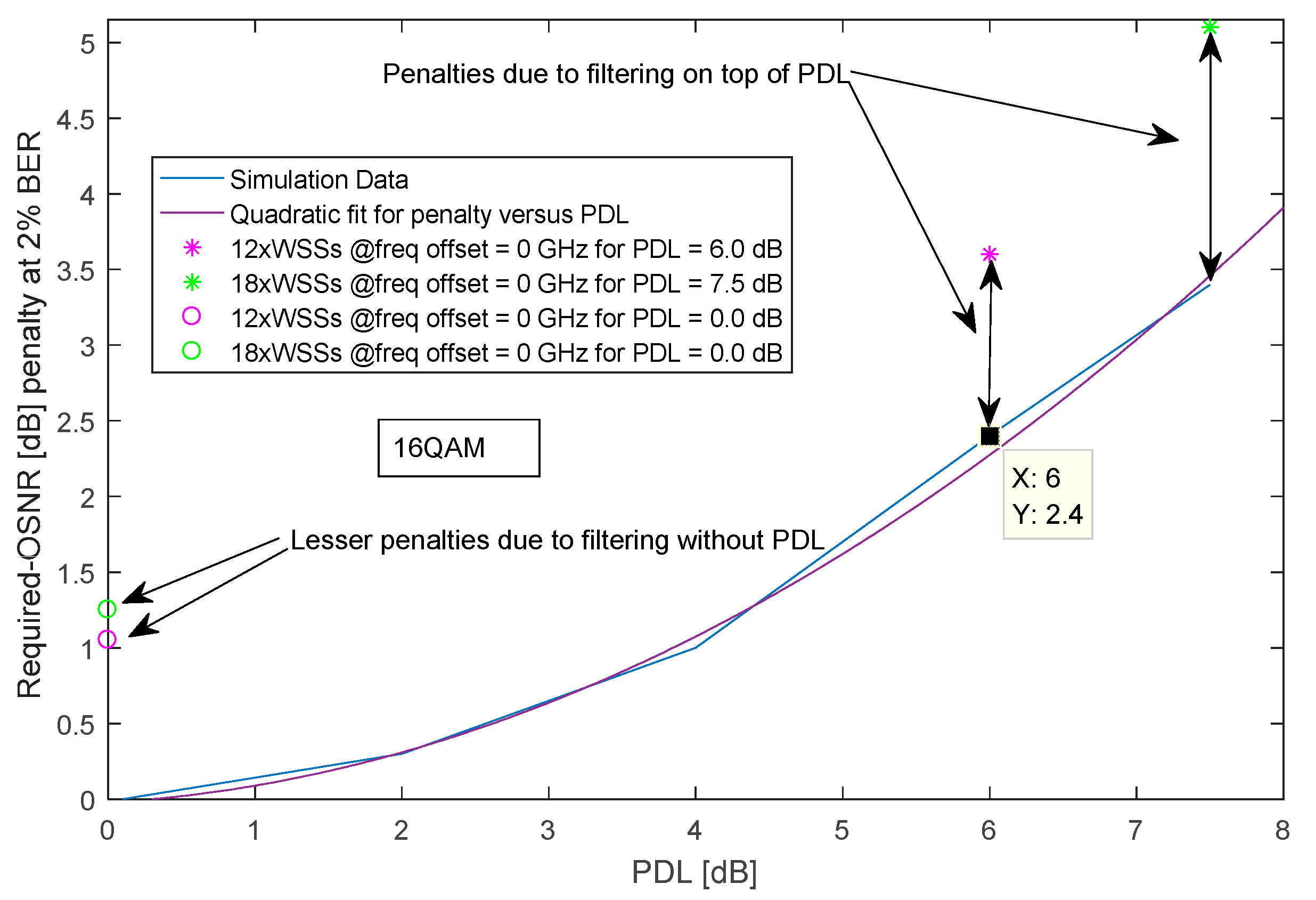
  • Continuously moving the compensation of the static portion of the channel, such as chromatic dispersion as in [22], from the adaptive filter to the static filters of the Tx and Rx, allows some of the adaptive filters taps to deal with more dynamic impairments of the optical link such as PMD and PDL. In other words, the saving in ROSNR can be used to tolerate an increase in PDL or more tracking of SOP.

7.3. Comparison of Experiments and Simulations Results

The lab results are shown in Figure 7a. Unlike how data displayed in presented simulation results, the required-OSNR again was measured per frequency offset and only the difference to post-compensation only is presented. We saw a consistent gain for both pre-compensation and proposed method, with the minimum gain equal to 0.2 dB, compared to Rx doing the full post-compensating using its adaptive filtering. The proposed method has a steady gain over pre-compensation. It does tell that the real-time transponder has many sources of noise on the Tx side. The simulation and lab results agree qualitatively. We will list some of the main differences between the two setups:
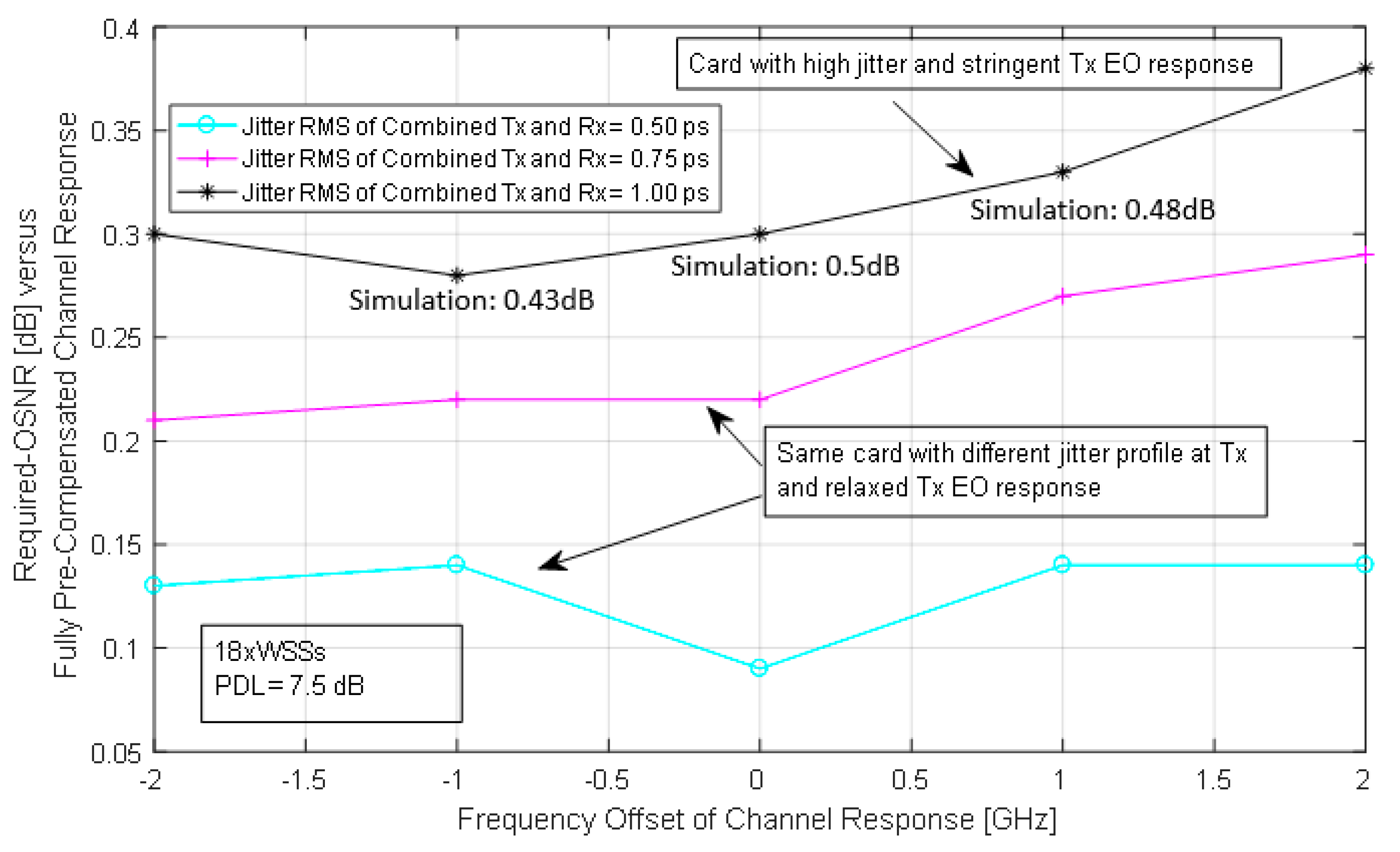
  • Although the Tx/Rx used in the simulation were fixed-point models with inherited implementation noise, other noise sources such as EO thermal noise were not captured. As well, since we are using 16QAM as modulation format, there is sensitivity of the results to In-Phase/Quadrature-Phase imbalance in power and delay. As well, it was not possible to simulate the same jitter profile generated by local VCO at both the DAC and ADC.
  • The resolution of the waveshaper does not permit the accurate replication of filters shapes (measured with spectrum analyzer with 400 MHz resolution). While in simulation, the channel model was done in floating-point.
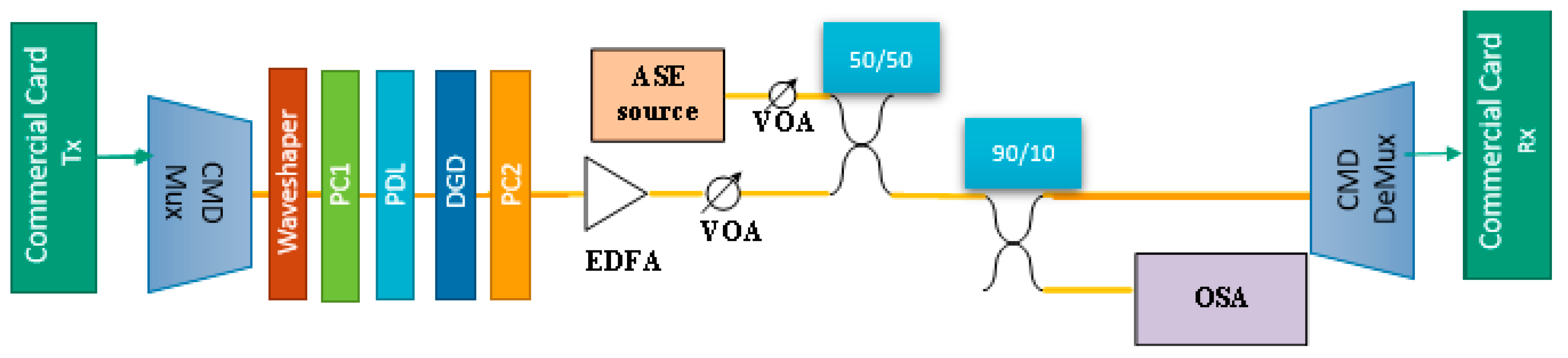
  • The EO model in the simulation had no ripples, while it can be seen from Figure 3b, when bypassing the waveshaper that the signal has frequency-dependent ripples.
  • Carrier recovery is activated in a commercial card, although the frequency difference between the Tx and Rx lasers was within 200 MHz from the ITU center frequency, the small dithering and phase noise would impact slightly (less than 0.025 dB compared to using one card in loopback—i.e., same laser) the results.

8. Conclusions

We presented a new method to perform an adaptive joint Tx/Rx compensation, of stringent filtering effected caused by CMDs and ROADMs in fixed-grid optical networks while using typical HW blocks in a coherent transponder. When the Rx filtering is not matched to the Tx pulse shape and the optical channel, this can result in insufficient electrical bandwidth and noise enhancement. The proposed method leverages Tx and Rx static filters compensation capability, of the channel frequency response, such that they effectively constitute a matched filter pair hence maximizing SNR at the input of the Rx adaptive filters [54,55]. With the filtering models representing real optical links and components, as well as the emulation of PDL, we showed an improvement in overall system performance. We showed for the first time, to the best of our knowledge, that splitting the compensation of heavy filtering in real deployment scenarios is better than doing only Tx pre-compensation or only Rx post-compensation. That is especially the case in presence of realistic implementation noise profiles at Tx, such as jitter at DAC, limited ENOB of DAC, clipping of filter coefficients and noise in the analog chain. With the 18xWSSs scenario, the simulation showed gain of up to 0.6 dB in the linear operation region and 1.1 dB in the nonlinear operating region. Lab measurements confirmed the method advantage in linear operating region by up to 0.4 dB.

Author Contributions

A.A. and C.D. conceived the idea and performed simulations and measurements. As well, analyzed the data and wrote the paper. All authors have read and agreed to the published version of the manuscript.

Funding

This work was funded by Natural Sciences and Engineering Research Council of Canada (NSERC) Grant #211300.

Conflicts of Interest

The authors declare no conflict of interest.

References

  1. Zhou, X.; Birk, M. Performance comparison of an 80-km-per-span EDFA system and a 160-km hut-skipped all-Raman system over standard single-mode fiber. J. Lightwave Technol. 2006, 24, 1218–1225. [Google Scholar] [CrossRef]
  2. Baxter, G.; Frisken, S.; Abakoumov, D.; Zhou, H.; Clarke, I.; Bartos, A.; Poole, S. Highly programmable wavelength selective switch based on liquid crystal on silicon switching elements. In Proceedings of the 2006 Optical Fiber Communication Conference and the National Fiber Optic Engineers Conference, Anaheim, CA, USA, 5–10 March 2006; p. 3. [Google Scholar]
  3. Marom, D.M.; Neilson, D.T.; Greywall, D.S.; Pai, C.S.; Basavanhally, N.R.; Aksyuk, V.A.; López, D.O.; Pardo, F.; Simon, M.E.; Low, Y.; et al. Wavelength-selective switches using free-space optics and MEMS micromirrors: Theory, design, and implementation. J. Lightwave Technol. 2005, 23, 1620–1630. [Google Scholar] [CrossRef]
  4. Filer, M.; Tibuleac, S. N-degree ROADM Architecture Comparison: Broadcast-and-Select Versus Route-and-Select in 120 Gb/s DP-QPSK Transmission Systems. In Proceedings of the Conference on Optical Fiber Communication, San Francisco, CA, USA, 9–13 March 2014. [Google Scholar]
  5. Zong, L.; Veselka, J.; Sardesai, H.; Frankel, M. Influence of Filter Shape and Bandwidth on 44 Gb/s DQPSK Systems. In Proceedings of the Optical Fiber Communication Conference and National Fiber Optic Engineers Conference, San Diego, CA, USA, 22–26 March 2009. [Google Scholar]
  6. Ghazisaeidi, A.; Tran, P.; Brindel, P.; Bertran-Pardo, O.; Renaudier, J.; Charlet, G.; Bigo, S. Impact of Tight Optical Filtering on the Performance of 28 Gbaud Nyquist-WDM PDM-8QAM over 37.5 GHz Grid. In Proceedings of the Optical Fiber Communication Conference, Anaheim, CA, USA, 17–21 March 2013. [Google Scholar]
  7. Tibuleac, S. ROADM Network Design Issues. In Proceedings of the Optical Fiber Communication Conference and National Fiber Optic Engineers Conference, San Diego, CA, USA, 22–26 March 2009; pp. 1–48. [Google Scholar]
  8. ROADMs & Wavelength Management, 1x9/1x20 Flexgrid Wavelength Selective Switch. Available online: https://www.finisar.com/roadms-wavelength-management/10wsaaxxfll (accessed on 11 August 2018).
  9. Krause, D.J.; Jiang, Y.; Cartledge, J.C.; Roberts, K. Pre-compensation for Narrow Optical Filtering of 10-Gb/s Intensity Modulated Signals. IEEE Photonics Technol. Lett. 2008, 20, 706–708. [Google Scholar] [CrossRef]
  10. Jiang, Y.; Tang, X.; Cartledge, J.C.; Roberts, K. Pre-compensation for the effects of cascaded optical filtering on 10 Gsymbol/s DPSK and DQPSK signals. In Proceedings of the 2009 35th European Conference on Optical Communication, Vienna, Austria, 20–24 September 2009; pp. 1–2. [Google Scholar]
  11. Pan, J.; Tibuleac, S. Real-time ROADM Filtering Penalty Characterization and Generalized Pre-compensation for Flexible Grid Networks. IEEE Photonics J. 2017, 9, 1. [Google Scholar]
  12. Pan, J.; Tibuleac, S. Real-time pre-compensation of ROADM filtering using a generalized pre-emphasis filter. In Proceedings of the 2016 IEEE Photonics Conference, Waikoloa, HI, USA, 2–6 October 2016; pp. 548–549. [Google Scholar]
  13. Foggi, T.; Colavolpe, G.; Bononi, A.; Serena, P. Overcoming filtering penalties in flexi-grid long-haul optical systems. In Proceedings of the 2015 IEEE International Conference on Communications, London, UK, 8–12 June 2015; pp. 5168–5173. [Google Scholar]
  14. Rahman, T.; Napoli, A.; Rafique, D.; Spinnler, B.; Kuschnerov, M.; Lobato, I.; Clouet, B.; Bohn, M.; Okonkwo, C.; De Waardt, H. On the Mitigation of Optical Filtering Penalties Originating From ROADM Cascade. IEEE Photonics Technol. Lett. 2013, 26, 154–157. [Google Scholar] [CrossRef] [Green Version]
  15. Gnauck, A.; Garrett, L.; Danziger, Y.; Levy, U.; Tur, M. Dispersion and dispersion-slope compensation of NZDSF over the entire C band using higher-order-mode fibre. Electron. Lett. 2000, 36, 1946. [Google Scholar] [CrossRef]
  16. Idler, W.; Buchali, F.; Schmalen, L.; Schuh, K.; Buelow, H. Hybrid Modulation Formats Outperforming 16QAM and 8QAM in Transmission Distance and Filtering with Cascaded WSS. In Proceedings of the Optical Fiber Communication Conference, Los Angeles, CA, USA, 22–26 March 2015; pp. 1–3. [Google Scholar]
  17. Pal, B.; Zong, L.; Burmeister, E.; Sardesai, H. Statistical Method for ROADM Cascade Penalty. In Proceedings of the National Fiber Optic Engineers Conference, San Diego, CA, USA, 21–25 March 2010; pp. 1–3. [Google Scholar]
  18. Pulikkaseril, C.; Stewart, L.A.; Roelens, M.A.F.; Baxter, G.W.; Poole, S.; Frisken, S. Spectral modeling of channel band shapes in wavelength selective switches. Opt. Express 2011, 19, 8458–8470. [Google Scholar] [CrossRef] [Green Version]
  19. Roudas, I.; Antoniades, N.; Otani, T.; Stern, T.; Wagner, R.; Chowdhury, D. Accurate modeling of optical multiplexer/demultiplexer concatenation in transparent multiwavelength optical networks. J. Lightwave Technol. 2002, 20, 921–936. [Google Scholar] [CrossRef]
  20. Ghazisaeidi, A.; Bigo, S.; Charlet, G.; Salsi, M.; Tran, P.; Renaudier, J. System Benefits of Digital Dispersion Pre-Compensation for Non-Dispersion-Managed PDM-WDM Transmission. In Proceedings of the 39th European Conference and Exhibition on Optical Communication (ECOC 2013), London, UK, 22–26 September 2013; pp. 1–3. [Google Scholar]
  21. Fan, Y.; Chen, X.; Zhou, W.; Zhou, X.; Zhu, H. The Comparison of CMA and LMS Equalization Algorithms in Optical Coherent Receivers. In Proceedings of the 2010 International Conference on Computational Intelligence and Software Engineering, Chengdu, China, 23–25 September 2010; pp. 1–4. [Google Scholar]
  22. Xie, C.; Winzer, P.J. Increasing Polarization-Mode Dispersion Tolerance of Coherent Receivers by Joint Optimization of Chromatic Dispersion and Butterfly Equalizers. In Proceedings of the Signal Processing in Photonic Communications 2013, Rio Grande, PR, USA, 14–17 July 2013. [Google Scholar]
  23. Viterbi, A. Nonlinear estimation of PSK-modulated carrier phase with application to burst digital. Trans. IEEE Trans. Inf. Theor. 1983, 29, 543–551. [Google Scholar] [CrossRef]
  24. Mizuochi, T.; Miyata, Y.; Kobayashi, T.; Ouchi, K.; Kuno, K.; Kubo, K.; Shimizu, K.; Tagami, H.; Yoshida, H.; Fujita, H.; et al. Forward Error Correction Based on Block Turbo Code With 3-Bit Soft Decision for 10-Gb/s Optical Communication Systems. IEEE J. Sel. Top. Quantum Electron. 2004, 10, 376–386. [Google Scholar] [CrossRef]
  25. Yang, W.; Kelly, D.; Mehr, L.; Sayuk, M.; Singer, L. A 3-V 340-mW 14-b 75-Msample/s CMOS ADC with 85-dB SFDR at Nyquist input. IEEE J. Solid-State Circuits 2001, 36, 1931–1936. [Google Scholar] [CrossRef]
  26. Equalizing Techniques Flatten DAC Frequency Response”, Maxim Integrated Application Note. Available online: https://www.maximintegrated.com/en/app-notes/index.mvp/id/3853 (accessed on 23 January 2020).
  27. Bachim, B.L.; Gaylord, T.K. Polarization-dependent loss and birefringence in long-period fiber gratings. Appl. Opt. 2003, 42, 6816–6823. [Google Scholar] [CrossRef] [PubMed] [Green Version]
  28. Tibuleac, S.; Filer, M. Transmission Impairments in DWDM Networks With Reconfigurable Optical Add-Drop Multiplexers. J. Lightwave Technol. 2009, 28, 557–598. [Google Scholar] [CrossRef]
  29. Vaseghi, S.V. Advanced Digital Signal Processing and Noise Reduction, 2nd ed.; Wiley: Hoboken, NJ, USA, 2008; ISBN 978-0-470-09495-2. [Google Scholar]
  30. Wiener, N. The Extrapolation, Interpolation and Smoothing of Stationary Time Series; OSRD 370; MIT: Cambridge, MA, USA, 1942. [Google Scholar]
  31. Kay, S. Fundamentals of Statistical Signal Processing-Estimation Theory; Prentice-Hall: Upper Saddle River, NY, USA, 1993; p. 386. [Google Scholar]
  32. Nelson, L.E.; Birk, M.; Woodward, S.L.; Magill, P. Field measurements of polarization transients on a long-haul terrestrial link. In Proceedings of the IEEE Photonic Society 24th Annual Meeting, Amsterdam, The Netherlands, 9–13 October 2011; pp. 833–834. [Google Scholar]
  33. Delesques, P.; Awwad, E.; Mumtaz, S.; Froc, G.; Ciblat, P.; Jaouën, Y.; Rekaya, G.; Ware, C. Mitigation of PDL in Coherent Optical Communications: How Close to the Fundamental Limit? In Proceedings of the European Conference and Exhibition on Optical Conference, Amsterdam, The Netherlands, 16–20 September 2012. [Google Scholar]
  34. Bertran-Pardo, O.; Zami, T.; Lavigne, B.; Le Monnier, M. Spectral engineering technique to mitigate 37.5-GHz filter-cascade penalty with real-time 32-GB aud PDM-16QAM. In Proceedings of the Optical Fiber Communication Conference, Los Angeles, CA, USA, 22–26 March 2015; pp. 1–3. [Google Scholar]
  35. Goebel, B.; Hellerbrand, S.; Haufe, N.; Hanik, N. PAPR reduction techniques for coherent optical OFDM transmission. In Proceedings of the 2009 11th International Conference on Transparent Optical Networks, Azores, Portugal, 28 June–2 July 2009. [Google Scholar]
  36. Pan, J.; Cheng, C.-H. Nonlinear Electrical Compensation for the Coherent Optical OFDM System. J. Lightwave Technol. 2010, 29, 215–221. [Google Scholar] [CrossRef]
  37. Hao, Y.; Li, Y.; Wang, W.; Huang, W. Fiber nonlinearity mitigation by PAPR reduction in coherent optical OFDM systems via biased clipping OFDM. Chin. Opt. Lett. 2012, 10, 010701. [Google Scholar]
  38. Chandrakar, U.O.; Bajpai, P.A.; Singh, R. Reduction of the nonlinearities by decreasing Peak to Average Power Ratio (PAPR) for Coherent Optical OFDM-WDM system using Exponential Compading. In Proceedings of the IEEE UP Section Conference on Electrical Computer and Electronics (UPCON), Allahabad, India, 4–6 December 2015; pp. 1–4. [Google Scholar]
  39. Krongold, B.S.; Tang, Y.; Shieh, W. Fiber nonlinearity mitigation by PAPR reduction in coherent optical OFDM systems via active constellation extension. In Proceedings of the 2008 34th European Conference on Optical Communication, Brussels, Belgium, 21–25 September 2008; pp. 1–2. [Google Scholar]
  40. Fraine, A.; Minaeva, O.; Simon, D.S.; Egorov, R.; Sergienko, A.V. Evaluation of polarization mode dispersion in a telecommunication wavelength selective switch using quantum interferometry. Opt. Express 2012, 20, 2025–2033. [Google Scholar] [CrossRef]
  41. Li, Y.; Gao, L.; Shen, G.; Peng, L. Impact of ROADM Colorless, Directionless, and Contentionless (CDC) Features on Optical Network Performance [Invited]. J. Opt. Commun. Netw. 2012, 4, B58–B67. [Google Scholar] [CrossRef]
  42. Braun, R.P.; Fritzsche, D.; Ehrhardt, A.; Schürer, L.; Wagner, P.; Schneiders, M.; Vorbeck, S.; Xie, C.; Zhao, Z.; Wan, W.; et al. 112 GBit/s PDM-CSRZ-DQPSK Field Trial Over 1730 km Deployed DWDM-Link. Opt. Soc. Am. 2010, 7988, 79880G. [Google Scholar]
  43. Santec Wavelength Selective Switch, Specifications in Brochure. 2012. Available online: https://www.santec.com/en/wp-content/uploads/edm_20121030_brouchure1.pdf (accessed on 20 January 2020).
  44. Sakamaki, Y.; Kawai, T.; Komukai, T.; Fukutoku, M.; Kataoka, T.; Watanabe, T.; Ishii, Y. Experimental demonstration of multi-degree colorless, directionless, contentionless ROADM for 127-Gbit/s PDM-QPSK transmission system. Opt. Express 2011, 19, B1–B11. [Google Scholar] [CrossRef]
  45. Wang, Q.; Yue, Y.; Yao, J.; Anderson, J. Adaptive Compensation of Bandwidth Narrowing Effect for Coherent In-Phase Quadrature Transponder through Finite Impulse Response Filter. Appl. Sci. 2019, 9, 1950. [Google Scholar] [CrossRef] [Green Version]
  46. Leeson, D.B. A Simple Model of Feedback Oscillator Noise Spectrum. Proc. IEEE 1996, 54, 329–330. [Google Scholar] [CrossRef] [Green Version]
  47. Mehrotra, A. Noise analysis of phase-locked loops. IEEE Trans. Circuits Syst. 2002, 49, 1309–1316. [Google Scholar] [CrossRef]
  48. Chen, L.; Tang, X.; Sanyal, A.; Yoon, Y.; Cong, J.; Sun, N. A 10.5-b ENOB 645 nW 100kS/s SAR ADC with statistical estimation based noise reduction. In Proceedings of the 2015 IEEE Custom Integrated Circuits Conference (CICC), San Jose, CA, USA, 28–30 September 2015; pp. 1–4. [Google Scholar]
  49. Chandrakasan, A.; Brodersen, R. Minimizing power consumption in digital CMOS circuits. Proc. IEEE 1995, 83, 498–523. [Google Scholar] [CrossRef] [Green Version]
  50. Sowailem, M.Y.S.; Hoang, T.M.; Morsy-Osman, M.; Chagnon, M.; Qiu, M.; Paquet, S.; Paquet, C.; Woods, I.; Zhuge, Q.; Liboiron-Ladouceur, O.; et al. 770-Gb/s PDM-32QAM Coherent Transmission Using InP Dual Polarization IQ Modulator. IEEE Photonics Technol. Lett. 2017, 29, 442–445. [Google Scholar] [CrossRef]
  51. Proakis, J.G. Digital Communications; McGraw Hill: New York, NY, USA, 1995. [Google Scholar]
  52. Abdo, A.; D’Amours, C. Adaptive Pre-Compensation of ROADMs in Coherent Optical Transponders. In Proceedings of the 2018 IEEE Canadian Conference on Electrical & Computer Engineering (CCECE), Quebec City, QC, Canada, 13–16 May 2018; pp. 1–4. [Google Scholar]
  53. Abdo, A.; Li, X.; Alam, S.; Parvizi, M.; Ben-Hamida, N.; D’Amours, C.; Plant, D. Partial Pre-Emphasis for Pluggable 400 G Short-Reach Coherent Systems. Future Internet 2019, 11, 256. [Google Scholar] [CrossRef] [Green Version]
  54. Kurosawa, N.; Kobayashi, H.; Kogure, H.; Komuro, T.; Sakayori, H. Sampling clock jitter effects in digital-to-analog converters. Measurement 2002, 31, 187–199. [Google Scholar] [CrossRef]
  55. Abdo, A.; Aouini, S.; Riaz, B.; Ben-Hamida, N.; D’Amours, C. Adaptive Coherent Receiver Settings for Optimum Channel Spacing in Gridless Optical Networks. Future Internet 2019, 11, 206. [Google Scholar] [CrossRef] [Green Version]
Figure 1. (a) ROADMs (reconfigurable optical add drop multiplexings) in typical networks configuration. (b) Signal with root-raised cosine (RRC) pulse shaping, as well, the two models used in simulation/experiment showing reduction in bandwidth due to cascaded 50 GHz ROADMs.
Futureinternet 12 00021 g001
Figure 2. Block diagram showing key functional blocks in coherent optical transponder and requirements for the operation of the presented method.
Futureinternet 12 00021 g002
Figure 3. (a) Common response of the adaptive filter after convergence; (b) Magnitude of common response for link scenarios.
Futureinternet 12 00021 g003
Figure 4. Simulated channel model with ROADM concatenation, noise and PDL.
Futureinternet 12 00021 g004
Figure 5. Required-OSNR penalty as function of PDL and filtering.
Futureinternet 12 00021 g005
Figure 6. Comparison of different compensation methods, for two links scenarios, in linear regime.
Futureinternet 12 00021 g006
Figure 7. Block diagram of experimental setup.
Futureinternet 12 00021 g007
Figure 8. Measured required-OSNR gain versus pre-compensation for different cards (with comparison to simulation).
Futureinternet 12 00021 g008
Figure 9. Impact on jitter with pre-compensation (i.e., more amplitude peaking at Tx) illustrated.
Futureinternet 12 00021 g009
Table 1. Fiber parameters.
ParametersSSMF Value
Span Length60 km
Kerr Coefficient 2.6 × 10⁻²⁰ m2/W
Dispersion16 ps/nm/km
Attenuation0.2 dB/km
EDFA Gain12 dB
EDFA Noise Figure6 dB
Laser Linewidth100 KHz

