Malware Classification Based on Shallow Neural Network

Abstract

The emergence of a large number of new malicious code poses a serious threat to network security, and most of them are derivative versions of existing malicious code. The classification of malicious code is helpful to analyze the evolutionary trend of malicious code families and trace the source of cybercrime. The existing methods of malware classification emphasize the depth of the neural network, which has the problems of a long training time and large computational cost. In this work, we propose the shallow neural network-based malware classifier (SNNMAC), a malware classification model based on shallow neural networks and static analysis. Our approach bridges the gap between precise but slow methods and fast but less precise methods in existing works. For each sample, we first generate n-grams from their opcode sequences of the binary file with a decompiler. An improved n-gram algorithm based on control transfer instructions is designed to reduce the n-gram dataset. Then, the SNNMAC exploits a shallow neural network, replacing the full connection layer and softmax with the average pooling layer and hierarchical softmax, to learn from the dataset and perform classification. We perform experiments on the Microsoft malware dataset. The evaluation result shows that the SNNMAC outperforms most of the related works with 99.21% classification precision and reduces the training time by more than half when compared with the methods using DNN (Deep Neural Networks).

1. Introduction

Malware has always been one of the main threats to cybersecurity, and the detection and analysis of malicious code has always attracted much attention. The number of new malicious code is growing at an alarming rate. According to AV-TEST, more than 4.62 million new instances of malicious code were detected from June 2019 to July 2019 [1]. However, few of the new malware have absolutely no connection to the early ones. A survey from Symantec pointed out that more than 98% of new malware is derived from existing malicious code [2]. Therefore, most of the new malware share similarities in their technologies or styles with some previously discovered malware [3], and such similar malware can be classified into the same family. For example, WannaCry, which broke out in May 2017, belongs to the same family as the Wcry malware that appeared in March of the same year. The variants of the former spread everywhere [4]. The classification of malware is helpful to study the evolution of the malware family and trace cybercrime, so it is important for preventing malware.

Malware analysis can be divided into two main categories: dynamic analysis and static analysis [5]. Dynamic analysis extracts features by executing malware in a controllable environment [6,7,8,9], which can observe the behavior of malicious code straightly. However, lots of manual effort is needed to perform dynamic analysis, and it is difficult to trigger all malicious behaviors [10]. In contrast, static analysis has higher analysis efficiency, but it relies on decompilation tools like IDA Pro [11,12,13]. Much information in the source code gets lost in the decompiling process. At the same time, encryption and obfuscation techniques also bring limitations to static analysis. In view of the characteristics of dynamic analysis and static analysis, static analysis is more suitable for the application scenario of our model, so the model proposed in this paper is based on static characteristics.

Several methods and techniques have been proposed to analyze malware with machine learning. In such methods, it is important to select the appropriate features and algorithms. Aiming at improving performance on unknown and evasive malware, Rong et al. [14] used pattern mining to obtain API (Application Programming Interface) sequences, and then the malicious API call sequences were used as abnormal behavior features to detect malware. Pajouh et al. [15] extracted the header information from the executable file on macOS, then analyzed the frequency of the base address offset, load instructions, the frequency feature of imported libraries and so on. Additionally, they used a support vector machine for malware detection. Nikola et al. started with the application permission information and executable file disassembly code [16], then built a feature model based on the bag-of-words model, which achieved a high detection accuracy on the Android platform. Aiming at the drawbacks of commonly used malware feature representation, such as variable length, high dimensional representation and high storage usage, Euh et al. [17] proposed low dimensional feature representation using WEM (Warning Electronic Module), API and API-DLL as an alternative scheme to ensure high generalization performance. However, machine learning-based methods require a great deal of expertise to perform artificial feature design, and these well-designed features may not be suitable for new malicious code, resulting in malware analysis becoming repetitive and time-consuming feature engineering work.

As an important branch of machine learning, a neural network can change the internal structure during training, and its adaptability helps to greatly reduce the labor cost in the design of feature expression. The neural network has attained remarkable achievements in the fields of machine vision and image recognition. In recent years, researchers have begun to introduce it into the field of malicious code analysis [18,19,20]. However, the existing work emphasizes the depth of the neural network. Although it has achieved good classification results, it also brings a whole host of problems, including parameters that are difficult to adjust, high calculation and storage cost and low analysis efficiency, which makes it difficult to apply to a scene with a huge amount of malicious code.

The existing work emphasizes the depth of the neural network, which brings some problems, such as parameters that are difficult to adjust, high calculation and storage costs and low analysis efficiency. This makes it difficult to apply to a scene with a huge amount of malicious code. The shallow neural networks usually tend to increase the width of the hidden layer (i.e., the number of neurons per hidden layer) to compensate for the reduced depth (i.e., the number of hidden layers). In turn, the shallow architecture has more parameters than the corresponding deep and narrow architecture for the same problem. G. E. Dahl [21] emphasized that using more hidden layers could not improve the accuracy. For example, a one-layer neural network performed better than two- and three-layer neural networks. The simplicity of a shallow neural network (SNN) allows for faster training, easier fine tuning and easier interpretation, and its effect can meet the application requirements. Thus, there is no need to consider deeper architectures.

In this paper, we present the shallow neural network-based malware classifier (SNNMAC), a model based on static features and shallow neural networks to classify a Windows malware sample to a known family. The classification of malicious code is helpful to analyze the evolutionary trend of malicious code families and trace the source of cybercrime. The SNNMAC extracts opcode sequences with the decompilation tool IDA and generates n-grams from the sequences. Then, a shallow network that consists of an embedding layer, a global average pooling layer and a hierarchical softmax layer will learn from the n-grams data set. Since malware always contains very long opcode sequences that generate a large number of n-grams, the SNNMAC uses an improved n-gram algorithm to leave fewer n-grams.

In summary, the main contributions of this paper are as follows:

• We propose a model based on shallow neural networks which can automatically learn from the raw data of malware samples, reducing a lot of manual feature engineering work;
• To avoid overfull parameters and huge calculation costs, we use the global average pooling layer and hierarchical softmax layer to take the place of the full connection layer and the softmax layer. This reduces computational complexity and avoids overfitting;
• We design an improved n-gram algorithm based on control transfer instructions. Compared with ordinary n-gram counts, our new algorithm generates fewer n-grams and reserves part of the original data’s structural information. It also reduces the training, detection time and storage space cost;
• We implement the SNNMAC and make a series of evaluation experiments for it. The results show that, when taking an n-gram count of 3-g, the SNNMAC achieves a classification precision and recall above 99%. At the same time, compared with other dense neural networks, the classification efficiency is higher, and the processing speed reaches 53 samples per second.

The rest of this paper is organized as follows. Section 2 describes the malicious code classification model based on shallow neural networks. Section 3 then discusses the experiments and evaluations, which include comparisons with other works. We conclude in Section 4 by doing a simple conclusion and identifying future work.

2. Related Work

Many previous works have proposed experiments that extract byte n-grams as features and have achieved high accuracies, which show that this is a reasonable and effective method [22,23]. J. Z. Kolter et al. [22] proposed a method using byte n-grams as a feature, combined with a gradient-boosting decision tree to perform malicious code classification tasks, and finally achieved a high true positive classification rate. Although it is an effective method to use a neural network on the basis of n-grams, it also inherits the disadvantages of byte n-grams, including the partial loss of character sequence information and the computational cost when n exceeds a certain value. Ö. A. Aslan and R. Samet [24] presented a detailed review on malware detection approaches and recent detection methods which use these approaches. Although the n-gram model has been widely used in malware detection, classification and clustering are more challenging for later processes because each continuous static and dynamic attribute is not related to each other. Therefore, in this work, we use the n-gram extraction algorithm based on control transfer instructions to reduce the size of the n-gram set while reserving part of the original data’s structural information.

In recent years, malicious code analysis methods based on machine learning and deep learning have been proposed. However, compared with the traditional machine learning algorithm, when the input data is large, a deep learning model can summarize the features by itself, thus reducing the incompleteness of artificial feature extraction. Haddadpajouh et al. [18] input opcode sequences as features to four kinds of LSTM-based deep networks for training and testing and compared the detection effect of LSTM under different parameters. Yan et al. converted malware binary files into grayscale images [19], combined with opcode sequences, and used CNN (Convolutional Neural Networks) and LSTM networks to learn the two features respectively before finally integrating the two outputs to get the final detection results. Liu et al. [20] proposed using GCN and CNN to process the API call graph and calculate the similarity between samples for malicious code family clustering. Raff et al. [25] proposed that a portable executable (PE) file could be regarded as a huge byte sequence, and it could be used as an input so that the deep learning model could learn its internal relations and features by itself. Vasan et al. [26] developed and tested a new image-based malware classification using CNN architecture integration, and their experiments proved that, compared with the traditional ML (machine learning)-based solution, it had great accuracy and avoided the manual feature engineering stage.

What we are interested in is that a neural network can learn feature representation from the original data, because this method not only improves the accuracy, but also reduces the domain knowledge. However, although the existing work has achieved good classification results, its emphasis on the depth of the neural network has caused a series of problems, such as high computational cost and low analysis efficiency. Therefore, we try to use the advantages of the shallow neural network model, such as faster training, easier fine tuning and easier interpretation, and apply it to a scene with a huge amount of malicious code. As far as we know, no other work has yet considered the use of shallow neural networks to classify malware.

3. Classification Methodology

Although it is an effective method to extract byte n-gram features, the standard n-gram algorithm treats all elements in the sequence equally, though not every assembly instruction is equally important to the program. Therefore, we needed an n-gram feature extraction method that considered the characteristics of a program’s structure.

Our second goal was a shallow neural network classification model with a high classification accuracy and processing speed. At present, more than 98% of new malware is derived from existing malicious code, and the number of malicious code is huge. Therefore, the classification of malicious code in the current environment requires both high accuracy and fast processing speed. We used the global average pooling layer and hierarchical softmax layer to take the places of the full connection layer and the softmax layer, which reduced the computational complexity and solved the problem of overfull parameters. Our strategy to achieve these goals can be divided into four steps. We will describe it in detail below.

3.1. Overview of Classification Model

The SNNMAC, the malware classification model we proposed in this paper, is for portable executable (PE) files, the binary executable file format on Windows. First, the SNNMAC disassembles malware sample files and extracts opcode sequences from the .asm file. Then, it applies the control transfer instruction-based n-gram on the sequences to obtain an n-gram dataset. Low-frequency word deletion and the hash trick are also performed in this step. Later, the embedding layer transfers every n-gram into a fixed-length vector, and the hidden layer produces a file feature for the output layer to decide the final label.

Concretely, the classification process of the SNNMAC can be divided into two stages. As shown in Figure 1, the first stage is to process the malware sample file. It generates n-gram data as the input of the next stage. The second stage takes a shallow neural network to learn from the n-grams and outputs the final classification result.

3.2. Opcode Sequences Process

The opcode sequence is a fine-grained feature that reflects the program logic and features. We used an IDAPython script to disassemble the PE samples in batches to get disassembled files in .asm format. Then, we traversed each line of the text section to fetch instructions.

The opcode sequences were very long. Taking the fonsiw malware family as an example, the average size of the binary files is 94 kb, but the average length of the extracted opcode sequence has reached 49,524. Such a large sequence is difficult to learn. We found that there were lots of assembler directives in the extracted instruction sequences, such as db, dd, area and align. Assembler directives only help the assembler to perform tasks during the assembly process, but do not generate any object code or affect program execution. Therefore, when extracting the sequence, these assembler directives can be filtered out to reduce the length of the opcode sequence. Staying with the fonsiw family example, after removing those instructions, the average length of the sequences is reduced to 23,719.

The opcode sequence extraction algorithm, described in pseudocode, is shown in Algorithm 1.

Algorithm 1. Opcode sequence extraction algorithm

Input: binary executive file Output: Opcode sequence asm_file = covert_to_asm(file) sequence = [] forlineinasm_file: opcode = line. split() if(opcode match regex)and(opcodenotpseudo_instruction): sequence.append(opcode) end if end for returnsequence

3.3. An Improved n-gram Algorithm Based on Control Transfer Instructions

The standard n-gram algorithm treats all elements in the sequence equally, but for the program, not every assembly instruction is equally important. The program execution flow is divided into many blocks by select statements, in which a sequence of statements is executed sequentially. Accordingly, the assembly code is divided into a number of basic blocks (BBLs) by the control transfer instructions. The basic block is the smallest unit of assembly codes, and many analysis processes translate the decomposing program into basic blocks as the first step [27]. A BBL is a single-entry, single-outlet instruction sequence. Considering the structural characteristics of programs, we propose a control transfer instruction-based n-gram (CTIB-n-gram) algorithm. Inspired by the concept of stop words in NLP (Natural Language Processing), we regarded the control transfer instructions in the sequences as delimiters. Only the n-gram starting with such instructions was reserved for representing the corresponding basic block, while all the other n-grams were dropped.

Each assembly instruction n-gram should be converted to a unique vector representation and added to subsequent training. However, as the number of samples and the size of n increases, the number of n-grams increases dramatically, and it is unrealistic to retain all n-grams. At the same time, the distribution of assembly instructions of n-grams is highly sparse, and some n-grams appear very infrequently, providing little information. The CTIB-n-gram algorithm filters the n-gram frequency below the set threshold and performs feature hashing on the n-gram set. Previous research [28,29,30] has shown that using feature hashing in multi-classification tasks, such as malicious code classification, helps to speed up training and avoid overfitting without causing a significant loss of precision.

The proposed CTIB-n-gram algorithm uses n-grams, starting with control transfer instructions, to express the corresponding basic blocks, then filters out the n-grams whose frequencies are lower than the threshold. Finally, the feature hash method is used to compress the set size. The n-gram set generated by the CTIB-n-gram algorithm is significantly smaller than the set obtained by the standard n-gram, which is helpful for accelerating the training and detection process. The pseudocode of the CTIB-n-gram algorithm is shown in Algorithm 2.

Algorithm 2. The proposed CTIB-n-gram algorithm

Input: opcode sequence, frequency threshold, number of hash buckets v Output: n-gram set V temp_set = [] forn-gramin sequence: ifn-gramstarts with[JMP, JNZ, LOOP, ...] temp_set.append(n-gram) end if end for forn-gramintemp_set: ifn-gram.frequency()<threshold: dropn-gram end if end for hash temp_set to v buckets V ← buckets returnV

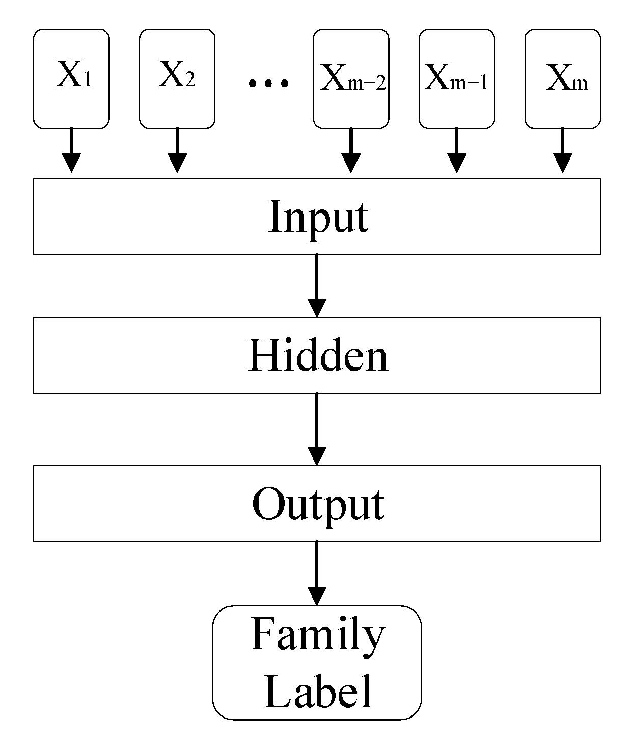
3.4. The Shallow Neutral Network

The shallow neural network used in this work was based on the classic continuous bag of words (CBOW) model, which consisted of an input layer, a hidden layer and an output layer, as shown in Figure 2.

3.4.1. Input Layer

After obtaining the n-gram set described above, one-hot encoding was performed first. One-hot encoding uses n-dimensional binary vectors to express n categories, and every vector has only a single 1 bit while all the other bits are 0. The one-hot encoding matrix is high-dimensional and sparse, requiring a lot of storage, and hence it is not convenient for direct calculation. Feature embedding, also called the decentralized representation of features, is a neural network-based feature representation method that maps high-dimensional vectors to low-dimensional spaces, thereby avoiding the curse of dimensionality and making it easier to learn from large inputs. Therefore, to map the one-hot encoding n-gram feature to the embedding feature vector, the model first performs feature embedding in the embedding layer, as shown in Figure 3.

The formula of the embedding layer is as follows:

$$H=X\cdot W$$

(1)

$X\in R^{m\times V}$ is the one-hot encoding matrix representation of the malware sample, where m is the number of n-grams extracted from the sample file and $V$ is the dimension of the one-hot encoding vector of each n-gram, which is also the number of hash buckets in the CTIB-n-gram algorithm described in the previous section. $W\in R^{V\times N}$ is the weight matrix maintained by the embedding layer, where $N$ is the specified feature vector dimension. At initialization time, the feature weight matrix $W$ is randomly generated and will be updated continuously during the training process. The output of this layer $H$ is an $m\times N$ matrix composed of the embedded vectors of all n-grams in the sample file and will enter the hidden layer.

3.4.2. Hidden Layer

The hidden layer of the model is a global average pooling (GAP) layer, which provides a fixed-size file feature vector for the output layer. The concept of the global average pooling layer was proposed in 2014 [31]. The GAP layer has no parameters, so it does not need to rely on special methods such as dropout to avoid overfitting. Compared with the fully connected layer, the GAP layer is more robust, faster and has no requirement for the size of the input matrix. As shown in Figure 4, the hidden layer projects each $m\times N$ matrix representing the sample file into a $1\times N$ vector.

The calculations performed at the hidden layer are as follows:

$$h=\frac{1}{m}{\displaystyle \sum _{i=1}^m{h}_i}$$

(2)

Each row of matrix $H$, denoted by $h_i\in R^N$, is an embedded vector of an n-gram in the sample. The GAP layer does not consider the order relationship between the n-grams extracted from the sample file; it directly calculates the sum of all the embedded feature vectors, and then averaging is performed to obtain the output $h$, which is the feature vector of the sample file.

3.4.3. Output Layer

Our model uses a hierarchical softmax layer to complete the final step in the family classification. Softmax is the most commonly used output function in multi-classification tasks. In a standard softmax regression, for each input, the probability of belonging to each class is calculated separately, and then the class with the highest probability is chosen as the output class label. As a result, when there are many class labels or the hidden layer output vector dimension is large, the calculation will be massive. Hierarchical softmax, based on the Huffman tree, transforms the multi-classification problem into multiple bi-classification problems. In the case where the family class number is k and the hidden layer output file feature vector dimension is d, the hierarchical softmax can reduce the computational complexity from $\mathrm{O}(kd)$ when using the standard softmax to $\mathrm{O}(d{\log }_{2}k)$ [32].

As shown in Figure 5, in the Huffman tree constructed by the output layer, the leaf nodes denote malware family labels, and the other nodes are called hidden nodes. When constructing a tree, the weight of each leaf node is the number of family samples in the training set, and the weight of the non-leaf node is the sum of the weights of all its child nodes. There is only one path from the root node to each leaf node that denotes a malware family. The output layer calculates the probability that a sample belongs to a certain family, according to this unique path. The probability of going to the right or left on every passing node will be multiplied. The formulas are shown below.

The probability of going left at node n, $P(n,left)$, is calculated as Equation (3) shows:

$$P(n,left)=\sigma ({\theta }_n^T\cdot h)$$

(3)

According to the nature of the activation function sigmoid, we can get the probability of going right at node n as in Equation (4):

$$P(n,right)=1-\sigma ({\theta }_n^T\cdot h)=\sigma (-{\theta }_n^T\cdot h)$$

(4)

Then, if we want to calculate the probability that the sample file expressed by the feature vector $h$ belongs to the malware family $c_1$ in Figure 3, the calculation is as follows:

$$P(c_1|h)=P(root,left)\cdot P(n(c_1,1),left)\cdot P(n(c_1,2),right)=\sigma ({\theta }_{root}^{}{}^T\cdot h)\cdot \sigma ({\theta }_{n(c_1,1)}^{}{}^T\cdot h)\cdot \sigma (-{\theta }_{n(c_1,2)}^{}{}^T\cdot h)$$

(5)

Extending to the general case, the probability of a malware sample expressed by vector $h$ belonging to family $c$ is calculated by Equation (6):

$$P(c|h)=\prod _{j=1}^{L(c)-1}\sigma (sign(c,j)\cdot {\theta }_{n(c,j)}^{}{}^{T}h)$$

(6)

where $L(c)$ is the unique path length from the root node to the leaf node of the class $c$, ${\theta }_{n(c,j)}^{}$ is the coefficient vector of the hidden node, whose transpose is ${\theta }_{n(c,j)}^{}{}^T$ and $\sigma$ is the activation function sigmoid.

Each hidden node vector is randomly initialized and updated with training feedback. Since the probability of the child node must be less than its parent node, when classifying a sample, we searched down along the branches having higher probabilities until the leaf node was reached, and then the corresponding label was obtained.

4. Experiments and Evaluations

4.1. System Implementation and Dataset

All experiments in this work were performed on a Mac mini PC.

Table 1. The platforms of the environment.

Platforms	Content
Hardware Dependencies	2.8 GHz Intel Core i5
	8 GB 1600 MHz DDR3
	Intel Iris 1536 MB
Software Dependencies	macOS Mojave 10.14.4
	Python 3.7.4
	Keras 2.0.9
	Numpy 1.16.2
	Pandas 0.24.2
	Scikit-learn 0.21.2
	Tensorflow 1.13.1

summarizes the major hardware and software platforms of the environment for the SNNMAC algorithm.

Due to the sensitivity of malicious code, the data sets used in most related works were not open to the public, and it is difficult to collect a large number of malware samples independently. Additionally, for the sake of the objectivity of the experiment, we used two data sets. The first data set was provided by the Microsoft Malware Classification Challenge (BIG 2015) [33], which contains 10,868 unique malware samples of 9 malware families on the Windows system. Each sample consisted of two files. One was a binary file without the PE header, and the other was the corresponding disassembly file generated by IDA Pro. The contents of the malware family samples are shown in

Table 2. The malware sample dataset (1).

Number	Malware Family Name	Sample Size
1	Ramnit	1541
2	Lolipop	2478
3	Kelihos_ver3	2942
4	Vundo	475
5	Simda	42
6	Tracur	751
7	Kelihos_ver1	398
8	Obfuscator.ACY	1228
9	Gatak	1013

. The second data set was obtained through the VirusShare website, including 8 families, 10,055 training samples and 1074 test samples. We used the open source tool AvClass to label the family names of malicious code and used an IDAPython script to disassemble the samples in batches and get disassembled files in .asm format. Then, we traversed each line of the .text, CODE and .code sections to fetch instructions. The contents of the malware family samples are shown in

Table 3. The malware sample dataset (2).

Number	Malware Family Name	Sample Size
1	Autoit	723
2	Delf	1847
3	Hotbar	1937
4	Onlinegames	2543
5	Sytro	1288
6	Fosniw	411
7	Renos	593
8	Installcore	713

.

We measured the following performance metrics in evaluation experiments: precision, recall and micro-f1. Micro-f1 is a generalization of the standard f1 value on the multi-classification tasks, and it treats multiple classifications as multiple bi-classifications. The metrics are defined as follows:

$$precision=\frac{TP}{TP+FP}$$

(7)

$$recall=\frac{TP}{TP+FN}$$

(8)

$$micro-f1=2\times \frac{precisio{n}_{sum}\times recal{l}_{sum}}{precisio{n}_{sum}+recal{l}_{sum}}$$

(9)

4.2. Experimental Results and Analysis

4.2.1. Model Performance

Table 4. The performance of the proposed model with 3-g.

Family Name	Precision	Recall	F1 Value
Ramnit	0.9677	0.9901	0.9788
Lollipop	0.9992	0.9976	0.9984
Kelihos_ver3	1	1	1
Vundo	1	1	1
Simda	1	0.9091	0.9524
Tracur	0.9863	0.9796	0.9829
Kelihos_ver1	0.9974	0.9871	0.9922
Obfuscator.ACY	0.9825	0.9615	0.9719
Gatak	0.9951	0.9980	0.9965
weighted average	0.9921	0.9918	0.9920

and

Table 5. The performance of the proposed model with 3-g.

Family Name	Precision	Recall	F1 Value
Autoit	0.9924	1	0.9962
Delf	0.9343	0.9925	0.9625
Hotbar	1	1	1
Onlinegames	0.9961	0.9454	0.9701
Sytro	1	0.9956	0.9978
Fosniw	0.9841	1	0.9920
Renos	0.9905	0.9830	0.9867
Installcore	0.9969	0.9969	0.9969
weighted average	0.9844	0.9836	0.9837

respectively show the classification performance of the proposed SNNMAC model for two datasets when the n of the n-gram was three. In this experiment, we randomly selected 3000 samples as the training set and 6000 samples as the testing set. In the second data set, one tenth of the data set was randomly selected from each family as the testing set, and the n value of three was also selected for the experiment. For each family, there were only two results: belonging or not belonging to this family. The standard f1 value was used here.

Figure 6 and Figure 7 show visual representations of the classification result confusion matrix of two datasets. The confusion matrix is a special matrix used to show the result of multi-classification tasks, with each column representing the prediction class and each row representing the actual class. The matrix is normalized due to the big difference in the number of family samples.

The experimental results show that the SNNMAC algorithm obtained a good classification effect for most malware families. It achieved 100% classification precision on five families. For the first dataset, except for the Simba family with a small number of samples, it achieved an f1 value of 0.95 due to the low recall rate. All other malware families obtained an f1 value greater than 0.97, a classification precision above 96.7% and a recall rate more than 96.1%. For the second dataset, except for the Delf family attaining a precision value of 0.93 and the Onlinegames family attaining a recall value of 0.95, all other malware families obtained f1 values greater than 0.97, classification precisions above 98.4% and recall rates of more than 98.3%.

4.2.2. The CTIB-n-gram Algorithm

To verify the effectiveness of the proposed n-gram generation algorithm CTIB-n-gram, we conducted a malware family classification experiment with a series of n values from 1 to 6. For each n value, the standard n-gram method and CTIB-n-gram algorithm were used in the model to generate an n-gram dataset. Then, the dataset was input into our network, and the results were compared. In addition, the value of n would also have a great impact on the results. The experiments in this section also compared the classification effects of the models with different n values. Figure 8a–c show the comparison of the precision, recall and micro-f1 values.

Experiments were performed on n values from 1 to 6. When n = 1, it is equivalent to no n-gram model. Since the CTIB-n-gram algorithm only retained the control transfer instruction and discarded a large number of other instructions, the classification model using the CTIB-n-gram algorithm was worse than one with the standard n-gram. At n = 2, the precision of the two methods was close, and the one with the CTIB-n-gram algorithm had a higher recall rate. At n > 2, the model using the CTIB-n-gram algorithm exceeded the model using standard n-grams in all three indicators, and the gap increased with the growth of n. It was noted that as the n value grew, the indicators did not always grow or remain stable. In the model using the standard n-gram, the performance began to decline when n > 4. When using the CTIB-n-gram model, the recall rate also began to decrease at n = 6, but the decline was not significant. As the value of n increases, the more instructions an n-gram contains, the less it discards. This is because the CTIB-n-gram model retained the control transfer instructions, which divide the assembly code into many basic blocks. The basic block, the smallest unit of assembly code analysis, is a single-entry, single-outlet instruction sequence. Therefore, the model based on the CTIB-n-gram algorithm had a higher accuracy than the standard n-gram model.

In terms of efficiency, when the n value was 2, the 2-g dataset file generated by the standard n-gram method exceeded 2 GB. However, the model using the CTIB-n-gram algorithm took only about 140 MB for the 2-g dataset file and about 440 MB when n was 6, far less than the storage the standard n-gram method needs. Naturally, the smaller the data file, the shorter the whole time will be when the subsequent processing is the same. For the sake of time and storage cost, the classification model using n-gram generally adopts bigram or trigram, so the CTIB-n-gram method can effectively improve the effectiveness and efficiency of malware classification in practice.

4.2.3. Comparison with Other Works

This section describes several comparative experiments we carried out. The comparative experiment consisted of two groups. One group used the common classifier of machine learning to perform classification, including Naive Bayes (NB), logistic regression (LR), support vector machine (SVM), random forest (RF) and Xgboost. The other group used the algorithms in the following three relevant works: the method used by the team who won the first place in the Kaggle malware classification competition [34], which takes a grayscale image generated from the .asm file, header information and the opcode n-gram as features with random forest as the classifier; the MalNet deep learning model [19] proposed by Yan et al., which combines CNN and LSTM networks to deal with the static features of malicious code; and the method proposed by Hanqi Zhang et al. [35], which feeds feature vectors composed of the TF-IDF(term frequency–inverse document frequency) values of the n-gram to five machine learning classifiers.

The results are shown in

Table 6. The results of the comparative experiments.

Group	Method	Precision (%)	Recall (%)	Time (min)	F1 Value
Common Machine Learning Classifier	NB	70.21	70.06	16	0.9838
	LR	71.42	67.38	17	0.6934
	SVM	54.84	28.75	18	0.3772
	RF	84.46	82.34	16	0.8338
	XGB	85.13	72.02	22	0.7803
Methods in Related Works	Kaggle Winner	99.63	99.07	269	0.9920
	MalNet	99.14	97.96	164	0.9865
	Hanqi Zhang	92.13	90.64	24	0.9138
SNNMAC	SNNMAC	99.21	99.18	27	0.9886

.

The same training set and test set samples were used for each experiment. The metrics compared included classification precision, recall rate and time consumed, where the time referred to the test time and did not include the time spent in the decompilation process. The experimental results show that the SNNMAC model is superior to the common machine learning classifier in precision and recall rate. Compared with the related methods, the classification precisions and f1 values from the SNNMAC model were only slightly lower than the method of the Kaggle winner, but the training time was reduced greatly, which makes the SNNMAC model more suitable for a real antivirus scenario with a massive amount of malware.

5. Conclusions and Future Work

In this paper, we proposed a malware classification method called SNNMAC, which uses a shallow neural network to learn from the assembly instruction n-gram dataset, which was generated by an improved n-gram algorithm based on control transfer instructions. We used the SNNMAC algorithm to complete a malware classification experiment for 10,868 samples from 9 malware families, and it achieved 99.21% precision and a recall rate of 99.18%. We also made a malware family classification experiment for comparison with other related works, and the SNNMAC model outperformed most of the other works with 99.21% precision and reduced training time greatly, compared with the related work. In order to reflect the objectivity of the experiment, two datasets were used in the experiment. It is shown that our approach bridges the gap between precise but slow methods and fast but less precise methods in existing work. In addition, it is more suitable for scenes with huge amounts of malicious code.

The model proposed in this paper uses a single feature and does not perform well in an extremely unbalanced class. At the same time, this model relies on the assembly instructions obtained by disassembly, and it cannot effectively detect executable files processed by technologies such as packing.

In future work, multidimensional features will be selected to express code features more comprehensively and further improve the classification effect of malicious code. Additionally, we plan to evaluate the SNNMAC model against other, larger datasets.