1. Introduction
Mixed-Integer Linear Programming (MILP) is considered by George Dantzig, one of its creators, to be an art as much as it is science [
1], due to its ability to find optimal solutions for challenging optimization problems. Some MILP models for problems of interest may be quickly solved, while other “seemingly easy” problems of huge practical importance remain unsolved [
2], despite several decades of great efforts [
3]. It is unquestionable that MILP has been successfully applied to a wide range of applications, with an astounding success in some specific applications, such as the traveling salesman problem [
4]. We present novel possibilities of MILP applications within a recent and innovative field of interest: the blockchain technology.
Blockchain is a disrupting technology, with importance to financial applications and
trustless architectures, as a decentralized platform for cooperation between parties that do not trust each other. Among existing blockchains and Distributed Ledger Technologies (DLT), Bitcoin [
5] is the oldest and most successful case. Since its inception in 2008 by Satoshi Nakamoto, a consensus based on Proof of Work (PoW) has started on Bitcoin network and never stopped producing new information chunks, called
blocks, through computationally expensive tasks called
mining. Network consensus participants, or
miners, have to agree on which sequence of blocks deserves continuation and aggressively compete to quickly find a SHA-2 [
6] hash value that correctly matches and expands the
chain of blocks. Since each block
points to (includes a hash reference to) previous blocks, it is not possible to change past information without affecting the whole future chain of blocks. Through in-time participation of miners, the blockchain network is always able to generate new blocks, while keeping past information immutable. One fundamental feature of PoW-based consensus (or
Nakamoto Consensus) is that nodes may naturally disagree on the next block (since mining process may be completed at the same time, with different hashes on different nodes), but every node must select only one of these “paths” to follow, commonly resolving these
forks in a few blocks (the most
supported fork is maintained).
Each block aggregates a batch of operations, called
transactions. On Bitcoin, transactions typically represent asset transfers between involved parties (validated through elliptic curve cryptography [
7]), solving the challenging double-spending problem with a transparent and global public ledger. However, transactions and blocks could also contain more complex computations. In 2013, Ethereum [
8] project launched a blockchain capable of performing Turing-complete [
9] computations, also including a global storage system. The consensus system was the same as Bitcoin, including the PoW strategy. During the same year, Neo project [
10] gave its first steps (under the name
Antshares) towards the design of a Turing-complete blockchain with One Block Finality (1BF) consensus, without relying on a computationally expensive PoW. This consensus system was named Delegated Byzantine Fault Tolerance (dBFT), adding network voting mechanisms over the groundbreaking work of Castro and Liskov [
11], the Practical Byzantine Fault Tolerance (PBFT).
The fundamental aspect of PBFT over other fault-tolerant consensus such as Paxos [
12], is that PBFT allow resistance to malicious agents, or
Byzantine, as named on the classic Byzantine generals problem [
13]. This allows a set of
nodes, typically named
Consensus Nodes, to cooperate and agree on a total-order of events, despite intentional and non-intentional failures up to
f simultaneous nodes. These ideas were soon adapted for the context of DLTs and blockchain [
10]. On dBFT, the consensus nodes cooperate via a Peer-to-Peer (P2P) network, collecting transactions submitted by nodes and organizing them in a memory pool mechanism (
mempool). The chain of blocks is formed in a linear manner, so each block is assigned with a unique incremental number, called
block index, where the largest block index in a chain of blocks is called
blockchain height.
The dBFT is a partially-synchronous algorithm, where each consensus node is allowed to temporarily become a
speaker in a round-robin fashion (see [
14] for more details). Given a height
H, consensus node
i will be declared speaker when
. The speaker node is allowed to propose a block (by grouping the transactions from its mempool), which is then validated by the other consensus nodes (at least
, since
f could have failed). If speaker does not respond (or appear to have failed), a timer is triggered after
T seconds and a
view change occurs, where consensus nodes nominate
as the next speaker. In theory, due to the 1BF nature of dBFT, only a single block can exist at each block height, and malformed blocks are rejected by the functional nodes, up to the Byzantine fault limit
f. To reduce the number of messages in P2P layer, the first version of dBFT (named dBFT 1.0) included only two of the three phases from PBFT, which allowed rare (but inconvenient) scenarios where more than one block is proposed (due to severe delays and timing issues). This situation required nodes to be reset after several weeks of operation, since following a “bad path” in the blockchain (also called
spork) would lock that node forever (no fork is possible in a 1BF consensus). A solution to this spork issue was made possible in 2019 with the proposal of dBFT 2.0, which included an extra
commit phase to the consensus, with other synchrony conditions. However, although operational in practice for several months (without any spork), no theoretical study has demonstrated the correctness of such mechanism. In fact, most consensus mechanisms proposed for blockchains typically do not include mathematical proofs for correctness, as it is very challenging and time-consuming task, focusing only on computational experiments. Moreover, computational studies typically focus only on non-Byzantine failures, which are easier to analyze.
This work proposes a MILP model that behaves as a
very strong Byzantine adversary, capable of exploring many sorts of issues in the consensus algorithm, including arbitrary network delays and generating intentional failures in an
exact manner (finding a maximum-damage scenario). Although quite strong, the adversary is computationally-bound such that it is not capable of subverting cryptographic technologies involved and to generate exponential delays. We apply the proposed technique for the Neo dBFT 1.0 and 2.0, demonstrating the Byzantine failures in a graphical approach (to visually observe attack conditions). The limitations of the approach are also discussed, due to the time discretization techniques employed and high number of variables in the model, so efficient solvers and integer programming are needed. We refer the reader to the paper by Coelho et al. [
15] for more details on the dBFT paradigm and recent discussions on novel consensus algorithms for blockchain. To the best of our knowledge, this is the first time MILP is used to generate exact adversarial models for the verification of Byzantine consensus systems.
This paper is organized as follows.
Section 1 introduces the work and presents background for MILP and the dBFT consensus. Then,
Section 2 presents background on replicate state machines for Byzantine problems, the detailed operations for three-phase dBFT consensus and a few related works from the literature.
Section 3 proposes mathematical formulations to describe several adversarial conditions for dBFT 1.0 and 2.0. On
Section 4, we perform several experiments and analyze the scenarios with a developed graphical tool. Finally,
Section 5 concludes the work and presents future perspectives for the verification of Byzantine models using experimental tools.
2. Background and Related Work
State Machines (SM) are in the core of replicated byzantine fault tolerant algorithms. The idea of representing fault resistant systems over SM have coined the term
state machine replication [
16,
17], where transition functions over a state graph determine how the system evolves in time. This graph describes how the system can react in a fully distributed manner to ensure
safety and
liveness against attacks.
In this sense, the recent work of Araújo et al. [
18] presents a library for fast development of state machines and byzantine fault tolerance, named
libbft. The libbft is inspired by timed automata theory [
19] and uses efficient cross-language serialization technologies, being able to easily intercommunicate with prototype implementations in C++ and Golang. This work explores a modeling for Neo dBFT algorithm, describing the states of dBFT 2.0 in a transition graph (more details on
Section 2.5), according to the internal phases of the algorithm.
Castro’s PBFT and Neo’s dBFT share several similarities regarding the phase changing strategy, where asynchronous messages are broadcast (possibly with delays) and used by replicated machines to progress through internal phases. Three phases are named on dBFT: PrepareRequest, PrepareResponse and Commit (with similar names on PBFT). As demonstrated by Castro and Liskov [
20] in a arduous mathematical task, the three phases of PBFT guarantee global convergence despite
f failures, meaning that once a single honest node enters a
Commit phase, all other
honest nodes are guaranteed to enter that same phase and to attribute the same total-ordering value to that specific transaction (even if that takes a big amount of time). With a similar reasoning, the dBFT intends to
Commit a new block and prevent sporks at current blockchain height (although challenging to deal with inherent non-determinism on block creation, due to mempool dependence). We describe each of the three phases of dBFT 2.0.
2.1. Phase I—PrepareRequest
In this phase, nodes will wait for a PrepareRequest in order to emit a PrepareResponse message. The speaker node i, where , is determined according to blockchain height H and view number v (starting from for every new height). The speaker groups a set of transactions from its mempool to form a new block. It adds a random nonce to the block header and dispatches this header together with PrepareRequest including only the hash of each transaction (not the complete content). Every honest backup node which is in the same blockchain height and view will receive the PrepareRequest, verify if it contains all transactions from block header (otherwise it will request missing ones from P2P), and then it verifies the transactions and issue a PrepareResponse if it agrees with the proposal.
If this process is completed in less than seconds, it goes to Phase II, otherwise it skips to View Change.
2.2. Phase II—PrepareResponse
In this phase, nodes wait for PrepareResponse messages to emit a Commit message. The purpose of this phase is to sync nodes regarding the acceptance of a valid block proposal; thus, if it receives at least PrepareResponse (including PrepareRequest and its own message), then it issues a Commit message. Note that Commit message publishes its final signature to support that block proposal, which cannot be changed anymore in order to prevent sporks (even with view changes). If this process (including Phase I) is completed in less than seconds, it goes to Phase III, otherwise it skips to View Change.
2.3. Phase III—Commit
In this phase, nodes wait for Commit messages to perform a Block Relay. The purpose of this phase is to ensure that nodes will agree on the same block proposal regardless of view changes; thus, if it receives at least Commits (including its own), then it is certain that block is unique and issues a BlockRelay message (including all transactions and signatures).
If this process (including Phases I and II) is completed in less than seconds, it increments blockchain height and restarts at Phase I, otherwise it skips to View Change.
2.4. View Change
If speaker node is faulty (issuing a bad block proposal), or for some reason its messages do not arrive in time for other nodes (thus, nodes may infer that speaker is broken), nodes will start an exceptional phase, called View Change. If any non-committed node receives ViewChange messages at view v, it will increment view number to and restart at Phase I. This allows a failed speaker node i to be replaced by node j in the next consensus round, i.e., .
2.5. dBFT 2.0 Diagram
Figure 1 describes the dBFT 2.0 diagram, automatically generated by libbft.
Note that, besides some
conditions for a state transition, some transitions include
actions, such as sending a P2P message or resetting the clock
C. The final state is indicated in a double circle (where process restarts). The notation used is the same as proposed by Araújo et al. [
18].
Regarding the methodological aspects of this work, we provide a MILP model which is capable of representing Byzantine adversarial conditions. In the literature, this approach reminds the resolution of problems from Game Theory [
21]. Specifically, linear programming have been strongly used to deal with zero-sum games with mixed strategies, such as
“Stone, Paper, Scissors”, and
“Two-Finger Morra” [
22]. These problems, although quite basic compared to the current proposal, already give the directions for solving game theoretic problems with more complex approaches, which we apply for decentralized consensus using MILP. For a review of MILP and game theory, see the recent review of Zaman et al. [
23]. Nash equilibrium has been explored via MILP techniques [
24,
25] in the literature, but mostly focused on simulating sets of actions that autonomous agents can perform as behavior [
26]. In this sense, the proposed MILP-based methodology seems to be equal or even superior in complexity to the state-of-the-art, due to the large number of scenarios allowed (also called
strategies), resolved throughout an intensive discretization of a multi-agent based consensus simulation.
We then proceed to the proposed mathematical programming models that are able to validate byzantine behavior for dBFT, including network delays and full control of f nodes.
3. Formulation for the dBFT Consensus
The proposed MILP model is detailed following the same procedure of Coelho et al. [
27], in which the proposed model is defined in distinct subsection showing constraints related to different part of the involved logic. The model is based on a time-discretization strategy (see [
28], a MILP model in which decision making is done in a discretized manner to decide instants to charge or discharge batteries), where byzantine agents have the flexibility to decide when (and if) messages are received by the other party. This ability simulates delays for message broadcasts on a P2P mempool layer. Due to the partial-synchronous nature of the consensus, each phase of dBFT stipulates a maximum timeout, so that failed speakers may be replaced by other consensus nodes on the next view. Each view increases the timeout by an exponential factor, so that it becomes too costly for an attacker to delay a message over a vTery long time (with delays growing over a linear factor). This is the same assumption from PBFT [
11], and it is even more challenging to perform such attacks on a dynamic P2P network, as it would require controlling several independent nodes of the P2P infrastructure simultaneously, while the location of consensus nodes on dBFT is not made public [
15].
3.1. Sets and General Parameters
The following parameters were defined and considered by the model:
- N:
Number of Nodes, .
- f:
Maximum allowed faulty nodes, .
- M:
Safety level .
- :
Set of discretization schedules .
- :
Set of nodes .
- :
Set of honest nodes , where .
- :
Set of rounds/views .
3.2. Auxiliary and Decision Variables
The following decision variables used to provide a complete solution to the proposed model. We use same notation from directed graph theory, denoting superscript with the concept of origin/send (via P2P broadcast system) and superscript as sink/receive. We also consider speaker node and primary node to be synonyms.
- :
Binary variable indicates if node is primary/speaker node on ; otherwise is backup node.
- :
Binary variable indicates if node sent a message at time on view .
- :
Binary variable indicates if node received a message from node time on view .
- :
Binary variable indicates if node sent a message at time on view .
- :
Binary variable indicates if node received a message from node time on view .
- :
Binary variable indicates if node sent a message at time on view .
- :
Binary variable indicates if node received a message from node time on view .
- :
Binary variable indicates if node sent a message at time on view .
- :
Binary variable indicates if node received a message from node time on view .
- :
Binary variable indicates if node relayed a block at time on view .
Some auxiliary variables were made necessary for calculating for checking operational requirements, constraints or assist the computation of a desired indicator:
- :
Counts the number of received messages for a node on view .
- :
Tells if any blocks was relayed at view ;
3.3. Goals to Be Optimized
Objective function values are calculated in each of the following variables:
- 1. :
Number of blocks relayed considering all views and total simulation time.
- 2. :
Number of views/rounds effectively used, which is the number of agreed view changes.
- 3. :
Number of communications, i.e., sent (, , and ) and received (, , and ) messages.
The goal of Objective 1 is to guide if the model should maximize or minimize the numbers of produced blocks. When maximizing, if we want to ensure no sporks, it should be limited to one. When minimizing, the desired value is also to be kept to one, which would result in a conclusion that says that liveness of the model is preserved.
The parcel of Objective 2 guides the model to finish faster or slower, which would enforce more or fewer rounds, and it need M nodes to agree throughout payloads.
Finally, Objective 3 brings more chaos to the system by maximizing the number of received message, as well as optionally minimizing it.
Weights
are, respectively, associated with these objectives functions and varying these weights can results in different optimal solution, as explored in [
27,
28].
3.4. Model Constraints and Blockchain Operational Requirements
We define the model within the next five subsections.
Section 3.4.1 defines some sets of constraints used for initializing the decision variables at instant
.
Section 3.4.2 introduces constraints used to define an active Primary and encloses the logic for ensuring single Primary in a round-robin manner.
Section 3.4.3 presents essential constraints that defines when a node can receive a payload.
Section 3.4.4 introduces a special set of constraints dedicated to honest nodes only
, which limits their behavior in terms of responding to payloads and respecting states such as Committed and Changing View. Finally, the calculation of the objectives functions and some auxiliary constraints that are needed are presented at
Section 3.4.5.
3.4.1. Time Zero Constraints
The set of constraints detailed on Equation (
1) initializes all sends and relays with zero; analogously, Equation (
2) initializes all received variables (note that all these variables correspond to
, when process starts).
3.4.2. IsPrimary Constraints
Equation (
3) starts the simulation, forcing at least one random node to have
IsPrimary set to one. Equations (
4) and (
5) limit to a single primary per view and set nodes to be
IsPrimary only once during the whole simulation, respectively.
Equation (
6) ensures that views should not be jumped; a Primary can only exist if previous Primary was active. Equation (
7) enforces that Primary will only be active if enough Change View messages were received on the previous view; parcel
is a multiplicative that forces the number of received messages to be, at least,
M.
3.4.3. Messages/Payloads Constraints
Equation (
8) ensures that a
PrepareResponse message is only send if PrepareRequest was received in an instant before. A similar behavior is ensured for sending a Commit messages, but with a stricter need of
M previous
PrepareResponse messages to have been received, as in Equation (
9). Analogously, Equation (
10) limits this by demanding that, at least,
M Commit messages should had been received before relaying a block.
Equation (
11) limits that a node can send messages only once per view; constraints are generated for the following variables
equals
,
,
and
.
Following this reasoning, Equation (
12) automatically forces a node to receive a self-sent message. They are created for the following pairs (
,
) equal to
,
,
and
. The same pairs are applied for Equation (
13), which enables messages to be received by a node
i only when they were actually already sent by another node
j.
Since
PrepareRequest carries Primary’s preparation hash, it also acts as a
PrepareResponse for the Primary, as ensured at Equation (
14).
Payloads can be received only once per view (
is assigned to
,
,
and
), which is defined with constraints created following the logic of Equation (
15).
3.4.4. Honest Nodes Constraints
If all nodes were to be Byzantine, then the aforementioned constraints would be sufficient for the model. However, we assume that, at least,
will be honest, which will, consequently, respect the following constraints defined in Equations (
16)–(
24).
Honest nodes will not relay more than one block (Equation (
16)), and they will force a Primary to exist if they can prove that they have enough change view messages, as ensured in Equation (
17).
Honest nodes will try to perform its whole of sending
PrepareRequest when Primary (Equation (
18)) and also respond to received messages. Equation (
19) has four parameters (
) which are assigned to the following groups:
,
and
.
Honest nodes will not send payloads on a higher view if a certificate of previous view was not obtained, as iteratively created in Equation (
20) by setting variable
to
,
,
and
.
If a commit state is not achieved, honest nodes will emit a
Change View, ensured at Equations (
21) and (
22). The first one ensures that only for View 1 (the first view), while Equation (
22) has an additional parcel that avoids forcing an honest node to send a Change View if previous view was not active.
Equation (
23) links the following pairs of sending actions:
:
,
,
,
,
,
,
and
. Those constraints are created to ensure, for example, that Change View will lock honest nodes from sending
PrepareRequest,
PrepareResponse or
Commit. A similar lock is ensured for
Change View if the node has the committed in an instant before or relayed a block with
, which will also block an honest to send anything else. As should be noticed, the second parcel of the equation has a summation that limits
to be within the limits
.
The set of constraints created from Equation (
24) blocks an honest node to send packages if a block was relayed on view before or commit state was reached. For this purpose, the generic equation is used to create constraints for the following pairs of
:
,
,
,
,
,
and
.
3.4.5. Objective Function and Auxiliary Variables Calculation
To check if a block was relayed, we define the two sets of constraints presented in Equations (
25) and (
26).
Equations (
27)–(
29) present the computation of the three objective functions considered to be optimized by the model. These three equations compose the objective function (as in Equation (
30)) with respective weights
,
and
.
In the next section, we discuss several experiments using the structure of the presented model, including variations of weights and optimization directions (according to Byzantine attack goals).
4. Computational Experiments
An implementation of the proposed MILP models can also be found at
https://github.com/NeoResearch/milp_bft_failures_attacks/tree/master/dbft2.0. The models were implemented using Python-MIP [
29] and using AMPL [
30], in order to verify inconsistencies and discrepancies between implementations (both implementations of the MILP model, using AMPL and Python-MIP, resulted in the same LP, which optimized provided optimal solutions for the variants presented in this study).
To optimize the MILP model, two solvers were used: CBC (COIN-OR Branch-and-cut, version Trunk 28 May 2020) and GUROBI 9.0. CBC has achieved a remarkable performance among open-source solvers (Mittelmann, MILP benchmarks, May 2020:
http://plato.asu.edu/ftp/milp.html), while GUROBI is a state-of-the-art commercial optimizer. The considered system was a linux kernel 5.4.0-42 with 16GiB RAM, 128 GB SSD, on a Intel(R) Core(TM) i7-7500U CPU @2.70 GHz.
4.1. Problem Instance Generation
We used the following script in Python to generate the instances:
python3 dbft2.0_Byz_Liveness.py–maximization –w1 = 1000 –w2 = 100 –w3 = 0 –N = 7 –tMax = 5, where parameters
and
N were iterated. Some characteristics of the generated problems can be seen at
Table 1.
Table 1 describes parameters of
N varying from 4 to 19 (note that all must respect
structure), and time intervals
from 5 to 25. Since the models will allow communications happening in same time intervals (send and receive), this allows very compact models (with little
) and drastically reduced number of variables for optimization solvers. In any case, total number of variables is presented in Column
vars, while binary and integer variables are listed in Columns
binaries and
integers, respectively. The number of constraints, as well as their respective types (equality or inequality), are also presented on the table. To give an extra insight on the MILP problems generated, non-zero elements in optimization matrix are described in Column
nzs.For practical benchmarks and to allow future comparisons, we generated (and published together with generator code) twelve different base problems with several extra variations on weights and optimization directions, where the largest problems are typically much harder to solve due to the massive increase of variables and constraints in the model. Larger time intervals are useful to explore situations where the Byzantine agent (or optimization solver) tries to postpone all activities for the maximum time possible (thus maximizing the delays), while shorter time intervals may reduce execution time and also limit Byzantine ability and may eventually turn the problem infeasible on practice.
4.2. Exploring Minimization and Maximization Optimization Directions
An interesting feature of the proposed model is its flexibility in being Minimized or Maximized.
Table 2 summarizes some combinations of weights and optimization directions used to exemplify the extreme scenarios highlighted in this paper. Weights
,
and
are described at
Section 3.3.
As described on
Table 2, Scenarios P1 and P2 are maximization problems with
set to 1000, favoring a high value of
, with different values for
(100 and
) regarding objective
(that can be considered time-related, as it counts the number of successive views in the system). This allowed the experimentation of interesting scenarios, where Byzantine actors behave differently depending on the
cost/benefit from the combination of weights. Due to
, Objective
is only regarded in P4.
Table 2 scenarios were built from practical experimentation regarding PBFT and dBFT theory, when exploring (optimizing) the instances in
Table 1.
4.3. Initial Experiments with Cbc and Gurobi
We considered both solvers Cbc and Gurobi on initial experiments. On a small scenario with and , the open-source Cbc spent s to prove the optimality of a P1 scenario, while commercial solver (with academic license) Gurobi spent only s. On other small scenarios, Cbc was not able to prove optimality within a large time limit, while Gurobi managed to find the solutions quickly. For this reason, we focused on only using Gurobi for large instances, but this gives an interesting insight on the real challenge behind these problems, as it is likely that Gurobi managed to find solutions quickly due to its large repertory of auxiliary heuristic functions and optimization cuts.
For a realistic blockchain scenario, we highlight that the MainNet of Neo Blockchain (operational since 2016) uses nodes, thus making it hard to analyze the models only using Cbc solver. For and on Scenario P1, Cbc is unable to prove optimality in 600 s with initial bound kept as 7700, while Gurobi achieves optimality in 73.16 s. Again, this reinforces that problem is difficult and Cbc still manages to finds some solutions, but it cannot achieve the necessary optimality condition for the exact adversarial model.
4.4. Graphical Visualization
We developed a graphical tool that integrates with the MILP to visualize the output solution of the mathematical model, mapping each decision variable in a
N-lined message grid (one line for each consensus node), which evolves in time horizontally (from left to right). This diagram was inspired by the works of Castro and Liskov [
11] and Coelho et al. [
15]. Each phase of dBFT has different colors (blue, green and yellow, respectively) attributed to its messages, and view change messages are marked as red. This is very interesting to quickly understand the
intention of the Byzantine agent behind the MILP solver, so as to detect elaborate types of attack on the blockchain consensus that were not predicted before. As is standard, we consider the last
f nodes (last
f lines) to be the Byzantine nodes, while others are honest. All of the
N timelines execute in parallel, so that the MILP model can fully represent any asynchronous behavior, subject to the time discretization parameter
. We demonstrate the cleanest example in
Figure 2, consisting of Scenario P6 with
and
(solver took around 100 s).
4.5. Ensuring Packages Delivery
Some additional set of constraints were used in MILP variants, in order to analyze how the model would behave for extreme scenarios. In this sense, Equation (
31) can be created for the following pairs
:
1. ;
2. ;
3. ; and
4. .
During experiments, it was observed that by only enabling Property (
4) (receives ChView always when ChView is sent) and minimizing
, all commits will be relayed and lost (Byzantine agent will explore the fact that sent messages are not necessarily received, even for commits). On the other hand, by enabling it together with Property (
3), the model can only find
N rounds as a minimum (the Byzantine agent explores the fact the MILP model is limited in time, thus leaving required constraints to be satisfied only on last time and not being computed by objective function). Thus, by considering only Property (
4), the optimal solution of Case P3 is kept as 100, while enabling Property (
3) moves this optimal to 200 because honest nodes would necessarily receive their respective commits on View 1, and then the system needs to have one node isolated and use the Byzantine node potential to
pretend being dead on the next view (see
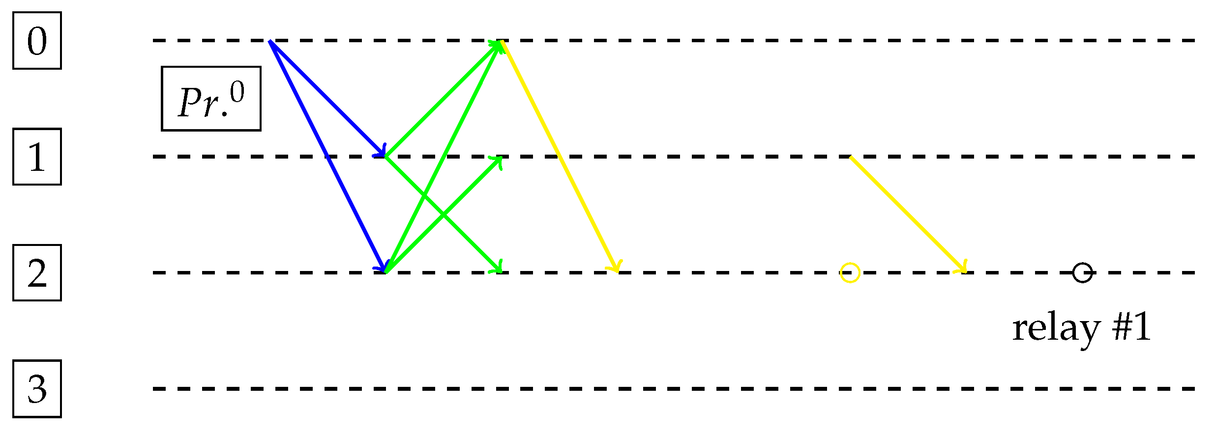
Figure 3).
In
Figure 3, the primary
(Byzantine)
luckily sends two successful PrepareRequest messages (in blue) to nodes 0 and 1 (but not 2), and then engages into a successful view change due to Property (
4). Node 1 is already committed at View 0, so it cannot agree on a new block for the next views. As time expires for View 0, honest backup
assumes as speaker (with support from nodes 2 and 3) and its new proposal is quickly resolved on View 1. In this case, no block is generated even if commits are received due to Property (
3). According to experiments, by enabling all sets of constraints created with Equation (
31), i.e., Properties (
1)–(
4), the optimal value becomes 1100. This happens as it becomes impossible to avoid the generation of a block due to the guarantee of message delivery between honest nodes.
In
Figure 4, any other Primary of the first round would have made the system relay a block on View 0. However, Byzantine was intrinsically part of the optimal solution (as first speaker) in order to maximize number of messages and number of rounds. Thus, the model was able to prove that liveness cannot be impaired if messages between honest are ensured.
Figure 5 graphically indicates the behavior of the Byzantine system on the P1 scenario. It maximizes the delays and blocks (trying to generate sporks), still being limited by the three-phase logic of the model (thus only generating a single block after all). The models finds a situation where the first primary
is Byzantine, so it does not propose a block and immediately requires a view change. The backup
assumes control after a view change, being able to propose a block (Phase I in blue), but unsuccessfully receiving responses in time. Since the delays cannot grow indefinitely (Byzantine agent is computationally bound as described on dBFT and PBFT specification), in the last view, the messages arrive and primary
is able to generate a relayed block (Phase 1 in blue, Phase II in green and Phase III in yellow). An interesting feature of the model is that it successfully maximizes its objective, such that the reception of some Phase I messages from
and
does not affect objective value (so as the
strange final relay participated by a Byzantine node). An optimal solution of cost 1400 is found, since a single block is produced (cost 1000) plus the maximum of four views (each costing 100). In
Figure 6, Byzantine nodes 5 and 6 are unable to affect anything, despite several tries with duplicated messages, and, since P5 maximizes the spent time, a complete solution to the problem (block generation) is only completely performed at last View 7.
4.6. Detected Problem Solving Limitations
The employed MILP technique allows modeling and quickly solving small-scale scenarios, while through usage of a commercial solver this limit has been fortunately expanded in order to demonstrate the correctness of a blockchain network with
nodes (which is the current size of the Neo MainNet, thus a practical proof for real-world scenario that is running nowadays). However, it is strongly desired that higher sets of nodes (
,
, etc.) are explored (see
Table 1), thus larger time discretization intervals. We believe that further advances in the topic may bring greater problem solving capabilities to the proposed MILP exact adversarial models, using hybrid exact and also metaheuristic techniques [
31].
5. Conclusions and Future Works
This work presents mixed-integer linear programming for exact adversarial model on a blockchain consensus. Blockchains are decentralized technologies that deal with many sorts of attacks, being both intentional (Byzantine) and non-intentional (general failures). We consider an application over the Neo Blockchain consensus, dBFT, which was inspired by the classical algorithm PBFT. Both PBFT and dBFT require that the number of Byzantine agents to be limited to f, from a set of consensus nodes. Since Byzantine agents may also provoke delays on the decentralized peer-to-peer network, we also model these delays in minimization or maximization scenarios, namely P1–P7, considering distinct constraints over message reception. We propose a set of instances with different sizes, varying number of nodes, and maximum time allowed for the system to exchange messages, which leads to the discovery of practical limitations on the power of open-source and commercial solvers to deal with these MILP problems. Finally, we present graphical tools to analyze the scenarios, demonstrating how Byzantine agents can explore every space of the MILP model, according to its own intention. To the best of our knowledge, this is the first work to successfully explore MILP exact models to find weakness on a blockchain consensus system, which we believe can help in the design of future consensus for large-scale public blockchain projects.
Several extensions are possible from this work, such as finding better algorithms to resolve MILP models of medium and large sizes (due to solver capabilities, we were limited to cases with few nodes and small time intervals); exploring how every pack of constraints affects the problem-solving capabilities of the solvers (including internal heuristics); extending current modeling to other recent blockchain consensus systems (including newer generations of Neo Blockchain consensus); developing real-time integration of the drawing tools with dynamic consensus simulations under the described adversarial conditions; and devising other exact adversarial conditions that may affect other families of consensus systems (e.g., purely asynchronous Byzantine agreements).

 ,
, 


