Abstract
Vehicle speed estimation is an important problem in traffic surveillance. Many existing approaches to this problem are based on camera calibration. Two shortcomings exist for camera calibration-based methods. First, camera calibration methods are sensitive to the environment, which means the accuracy of the results are compromised in some situations where the environmental condition is not satisfied. Furthermore, camera calibration-based methods rely on vehicle trajectories acquired by a two-stage tracking and detection process. In an effort to overcome these shortcomings, we propose an alternate end-to-end method based on 3-dimensional convolutional networks (3D ConvNets). The proposed method bases average vehicle speed estimation on information from video footage. Our methods are characterized by the following three features. First, we use non-local blocks in our model to better capture spatial–temporal long-range dependency. Second, we use optical flow as an input in the model. Optical flow includes the information on the speed and direction of pixel motion in an image. Third, we construct a multi-scale convolutional network. This network extracts information on various characteristics of vehicles in motion. The proposed method showcases promising experimental results on commonly used dataset with mean absolute error (MAE) as km/h and mean square error (MSE) as .
1. Introduction
Intelligent transportation systems (ITS) are of practical importance and interest for traffic regulators and supervisors. They provide support for government departments in traffic management, commuting improvement, traffic congestion relief, traffic accident prevention, etc. A critical component of traffic management practice and a popular topic in ITS research is vehicle speed estimation [1], which is widely applied to identify traffic congestion or other events of interest. In this paper, we focus on the average vehicle speed estimation problem, which is defined as the average speed of all the vehicles in a scene.
One family of approaches to vehicle speed estimation is based on additional specialized hardware. Three commonly used devices are induction-coil loop detectors, laser detectors, and radar detectors [2]. They all have shortcomings in practice. The inductive loop detector method requires installing a loop detector in the ground. The installation process is complex and can adversely affect road condition (accelerate asphalt deterioration) [3]. Laser detectors and radar detectors do not cause these problems, yet they need frequent and expensive maintenance. Furthermore, radar detectors need to be meticulously positioned in consideration of installation angle.
Another family of approaches to vehicle speed estimation is based on surveillance camera information. Nowadays, high-resolution digital cameras are ubiquitous, which provide economic and accessible sources of data. However, it is a challenging problem to extract relevant information on traffic form video footage [4]. A conventional practice for information extraction is to install two cameras in specifically chosen locations and process the data collected by the two cameras with particularly designed algorithms. In contrast, monocular cameras are not currently in extensive use for traffic information extraction. However, there are two primary benefits in using single monocular cameras. First, monocular cameras are standard infrastructure for most of the established surveillance camera systems. Thus, it does not require substantial investment in infrastructure. Second, monocular cameras have wider coverage compared to two-camera systems. In particular, monocular cameras can simultaneously monitor multiple lanes.
One existing monocular camera-based method to vehicle speed estimation utilizes the technique of Camera Calibration [1,5,6]. In short, this method obtains the algorithm-generated scale and calculates the speed based on the vehicle trajectories acquired by a two-stage process including detection and tracking. The camera calibration process require the input of the intrinsic and extrinsic parameters. Due to different camera models, shooting angles and installation positions, camera calibration is required for each camera. Some camera calibration-based methods need the multiple manual measurements on the road [5,7,8]. Some algorithms have limitations in camera placement [1,5,9,10]. Besides, the accuracy of the speed estimate heavily relies on the accuracy of algorithms for detection and tracking. A variety of suboptimal environments (illumination variation, motion blur, background clutter and overlapping, etc.) could result in problems in vehicle detection and tracking, including detection missing, false detection, tracking loss, etc. [11]. When the vehicle detection or tracking is subpar, the error of speed estimation will be significant. More detailed analyses are presented in Section 2.1.
As an attempt to ameliorate the aforementioned limitations of camera calibration- based methods, we propose an automatic approach to average vehicle speed estimation based on video footage. Figure 1 is a schematic illustration of our method. The inputs: RGB images and optical flow from a short video. The outputs: the average speed of the vehicles in the video. The input images only need to be standardized and scaled. RoI (Region of Interest) in images can be defined to do average vehicle speed estimation on a single lane. Our method has no limitation on the position of the camera installation, and it does not needs to know the parameters of the camera, nor to detect or track the vehicles. Given enough scenes covered by the constructed training set, we can estimate the vehicle average speed in any scene. Therefore, our method is simple to operate, with high maneuverability and wide application range.
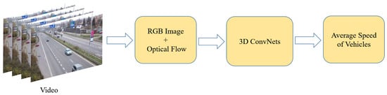
Figure 1.
Flow Chart of Our Method.
As with video action recognition, vehicle speed estimation task is also a problem about video understanding. Inspired by the successful application of 3D ConvNets in video action recognition, we use 3D ConvNets as the base model. The base model yields promising results on the test set with mean absolute error (MAE) as 2.73 km/h and mean squared error (MSE) as . Although numerical experiments suggest an inferior accuracy level of our method to that of hardware-based methods. Yet our method is sufficiently accurate for most practical purposes such as vehicle flow computation and traffic congestion identification.
Our work can be summarized as follows:
- We propose 3D ConvNets to estimate average vehicle speed based on video footage. In contrast to camera calibration-based methods, our method is an end-to-end method, independent of external factors. In particular, our method does not entail detecting or tracking vehicles.
- We propose to include non-local blocks so as to capture spatial-temporal information with a ‘global’ perspective.
- We propose to add optical flow from video as an input to the model. Optical flow contains useful information on the vehicle motion, which can be used to improve the model accuracy.
- We propose to employ the multi-scale convolution to extract the information of vehicles with different scales contours. This design resolves the problem of vehicle size varying due to their different distances from the camera.
2. Related Work
Deep learning has been extensively studied and applied as a high efficiency approach to a wide range of problems. In recent years, this method has brought revolutionary changes to the fields of image recognition [12], object detection [13], and video action recognition [14]. The success of 3D ConvNets application in video action recognition gives us inspiration to apply 3D ConvNets to average vehicle speed estimation. In this section, we present relevant academic work on vehicle speed estimation including camera calibration, video action recognition, and the non-local algorithm.
2.1. Methods Based on Camera Calibration
Methods that use camera calibration to estimate vehicle speed typically consist of the following steps:
- Camera Calibration: A projection matrix is obtained , where K represents intrinsic camera parameters, while R and T are extrinsic parameters, representing camera rotation and camera translation, respectively. The internal camera parameters related to the characteristics of the camera itself, such as the focal length, pixel of the camera. The external calibration parameters are the position and orientation of the camera relative to some fiducial coordinate system. The orientation of the camera often changes slightly due to weather and other reasons, so the parameters need to be reset frequently.
- Detection-Tracking: Detect the contours of the vehicle in the image; then track the vehicle by the detected contours. This step is to plot the trajectory of the vehicle on the road.
- Vehicle Speed Calculation: Calculate the traveling distance of the vehicle based on the information obtained at stage one and two. Trivially, measure the elapsed time during the traveling period. With the distance and time duration, calculate the vehicle speed by the basic formula: .
Camera Calibration-based methods can be categorized into semi-automatic and fully-automatic. In the first case, the computation is automatic except for the camera calibration part, where manual manipulation required is usually in the form of measuring certain distances in the scene and certain camera parameters. For example, Pin Hole Model [5] requires the camera height from the ground plane is used for camera calibration, and Gaussian Mixture Model and Kalman Filter are used for detection and tracking. Some methods make use of line markings on the road to deal with perspective projection [15,16,17]. In [18], the width of lane and road white strips length are essential information for camera calibration. In this study, Mask-RCNN and deep-SORT [19] are vehicle detector and tracker, respectively. Huang [4] uses warping with the linear perspective transformation to convert the distance from pixel to the real world. Besides, this study uses Faster R-CNN to do multi-object detection, and the tracking algorithm is based on histogram comparison. To sum up, some externally acquired information is necessary for semi-automatic camera calibration-based methods. Dubská et al. [20] present a fully-automatic method which is used for an arbitrary view. This method calibrates the camera by determining three vanishing points which define the stream of vehicles and then computes the 3D bounding box around the vehicle blobs. Finally, they use the Kalman Filter to track the 3D bounding box of the vehicle. Sochor et al. [21] improve the previous method based on two detected vanishing points. Besides, a multi-objective evolutionary algorithm is applied for camera calibration in [22], and vehicle tracking is done by license plate recognition.
In summary, methods based on camera calibration are highly dependent on external conditions and the effectiveness of detection and tracking algorithms [23]. Most of them require manual intervention and the camera can not be placed at any position above the road. Besides, because of the complex outdoor environment the parameters need to be reset frequently. Although deep learning significantly improves detection and tracking results, these two tasks still remain as challenges in practice. Especially when the traffic flow is large, the overlapping between vehicles is easy to occur, which makes the extracted feature information incomplete and incurs false detection, missing detection or tracking loss. Therefore, plotting vehicle motion trajectories with a satisfactory level of accuracy is challenging in complex and dynamic environments.
2.2. Video Action Recognition
The primary objective of Video Action Recognition is to identify human behavior from video footage. Naturally, it is sometimes referred to as Human Action Recognition. Some methods to average vehicle speed estimation entail video analysis, thus we borrow ideas from video action recognition models to apply to the vehicle speed estimation problem.
In particular, 3D ConvNets is very useful technique for capturing spatial-temporal features. In contrast to 2D ConvNets, 3D ConvNets, characterized by 3D convolution and 3D pooling in 3D ConvNets, can effectively capture spatial-temporal information. Specifically, 3D convolution is carried out by convolving a 3D kernel with a cuboid formed by several contiguous frames stacked together [24]. By this means, the motion and timing information in continuous frames can be extracted. Tran et al. [25] propose a C3D model that includes eight convolutions, five max-poolings, and two fully connected layers. This C3D model yields better results than 2D ConvNets in video action recognition. Inspired by the C3D model, 3D ConvNets have been extensively studied. Feichtenhofer et al. [26] propose Spatiotemporal Residual Networks which integrates two stream ConvNets [27] and 3D ResNet together. In [28], the R3D network is constructed based on ResNet [12]. Recognizing that temporal and spatial dimensions are not symmetric, Qiu et al. [29] propose a P3D model, and Tran et al. [30] propose a R(2+1)D model. Both models reduce 3D convolutions into 2D convolution operations in space domains and 1D convolution operations in time domains. This technique increases the non-linearity of the network and improves the performance compared to the original 3D ConvNets.
Even though 3D ConvNets can capture features and motion information encoded in image sequences, it is difficult to train the models due to the great number of parameters. In an effort to solve this problem [14], inflates 3D ConvNets (I3D). More specifically, it initializes the parameters of a model by inflating the 2D pre-trained weight from ImageNet to 3D. Subsequently, the pre-trained 2D kernel weights are repeated along the temporal dimension t times and rescaled by .
2.3. Non-Local Algorithm
The non-local algorithm [31] was initially designed for image denoising, which is carried out by averaging of all pixels in an image. It assign the distant pixels the same weights in computing the filtered responses. Subsequently, the Non-local mean technique was developed into block-matching 3D (BM3D) [32], which groups similar 2D image fragments (e.g., blocks) into 3D data arrays. Moreover, Wang et al. [33] pinpoint that non-local operations have a desirable feature of capturing long-range dependencies by computing interactions between any two positions, regardless of their positional distance. Thus, including non-local blocks into neural networks improves the result of image recognition, video action recognition, object detection, and so on. Particularly, self-attention [34] in machine translation is a specific form of non-local algorithm. Inspired by these works, we include non-local blocks into our model to effectively capture long-range dependencies between space and time.
3. Model
In this section, we describe the detailed configuration of spatial-temporal model and the flow of our method. According to the specifics of the actual application, we modify the 3D Resnet50 model in the following regards:
- Recognizing the asymmetry of the spatial and temporal information, we introduce (2+1)D convolution to more effectively extract the spatiotemporal features;
- We embed non-local blocks to the network to take into consideration ‘global’ information;
- We employ multi-scale convolution to better capture the information of vehicles’ varying sizes due to the varying distances between the vehicles and the camera.
Since average vehicle speed estimation is a regression problem, we use Mean Square Error as the loss function:
where N is the number of samples, while and are the estimated value and ground-truth of sample i, respectively. The loss is the mean of the squared Euclidean distances between all the real sample values and the predicted values.
We discuss the model in greater detail in the following part of the paper.
3.1. Inflated (2+1)D Convolution
In generally, 2D convolutions are applied to capture spatial features. In addition to spatial features, it is essential to consider the temporal relationship between frames. Conceptually, 3D convolution is achieved by convolving a 3D kernel to a cube that is formed by stacking multiple contiguous frames together [24]. Comparatively, 3D convolution is superior to 2D convolution in that 3D convolution can extract both spatial and temporal information, whereas 2D convolution can only extract spatial information. We use 3D ResNet50 to capture spatial-temporal features from videos.
3D ConvNets, like C3D [25], have significantly more parameters than the corresponding 2D ConvNets by reason of the new convolution kernel of the time dimension. With the large number of parameters, they are hard to train [14]. We attempt to work around this issue by inflating 2D convolution weights from ImageNet pre-training to 3D. We initialize all 3D convolution kernels with 2D convolution kernels, which are pre-trained on ImageNet. For instance, if a 3D convolution kernel size is , we initialize them by repeating the pre-trained 2D kernel weights along the temporal dimension t times and then rescale by .
The 2D convolution contains directions x and y. Roughly speaking, the step sizes in these two directions are the same (kernel size and stride). However, in 3D convolution, the time dimension cannot be reduced too fast or too slow because it relies on image dimensions and frame rates. If it changes too quickly relative to space in time, it may confuse the edges of different objects, thus undermining the early feature detection. If the time dimension changes too slowly, it may not be able to effectively capture the scene dynamics. With this tradeoff in mind, we set the kernel of the first convolution layer as ; the first Maxpooling layer’s kernel as , and the second Maxpooling layer’s kernel as .
Due to the asymmetry between time and space domains , the convolutions of these two domains are carried out separately [29,30]. The new spatial-temporal convolutional block is called (2+1)D Convolution. 3D convolution is solved with two consecutive operations: 1. a 1D temporal operation; 2. a 2D spatial operation. In other words, the spatial-temporal convolution consists of one temporal convolution and one spatial convolution. An illustration of this process is given in Figure 2. The full 3D convolution kernel size is , where t is the temporal width and k denotes the spatial width and height.
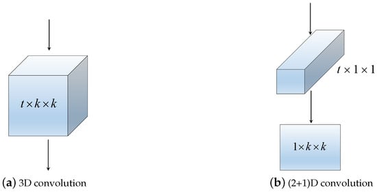
Figure 2.
3D Conv VS (2+1)D Conv.
Based on the aforementioned idea, continuous and convolutional kernels in 2D ResNet50 are changed into and in 3D. Table 1 shows the structural differences across the 2D ResNet, the R3D50, and the R(2+1)D50 network structures.

Table 1.
2D ResNet50 vs R3D50 vs R(2+1)D50.
3.2. Non-Local Blocks
The Non-local block expands the receptive field of the model to capture long-range dependency. We first present the mathematical expression for the non-local operation. Then, we detail how to add non-local blocks to our model.
A non-local operation computes the response in one position as a weighted sum of the features in all positions. According to the non-local methods [31,33], the generic non-local operation in neural networks is presented as:
where is the input signal, which could be in the form of images, sequences, and video features, while is the output signal of position i. f is a pairwise function that computes the correlation between and all . The function g conducts a transformation on . The summation of f and g is then normalized by a factor .
From Equation (2), we know that the non-local operation considers all position () of inputs. In contrast, a standard 1D convolution sums up the local neighborhood weight (e.g., , in the case of kernel size equal to 3), and the recurrent operation at time i is often based only on the current and the preceding time steps (e.g., or ).
There are several candidates for the pairwise function f, such as the Dot product, the Gaussian, and the Embedded Gaussian. According to the experiments in [33], the non-local models are not sensitive to the choice of f, so we randomly choose the Embedded Gaussian function for f. Mathematically:
Here, and are same in Equation (2). and are two embeddings. For the sake of brevity, we set g as a linear embedding, , where is a learned weight matric. Taken together, .
The non-local operation in Equation (2) is flexible and can be incorporated into any existing network architectures. We warp it into a non-local block as follows:
Here, is the same as Equation (2), and ‘’ denotes a residual [12]. Due to the residual connection, we can insert a non-local block into any pre-trained model without adversely affect its structure and results.
We include the non-local block in our model to capture more vehicle spatial-temporal features from video footage, as shown in Figure 3. X is the input tensor and Z is the output tensor. refers to the dimensions of the input tensor X. ’⊗’ represents the matrix multiplication, and ’⊕’ stands for the element-wise sum. The blue rectangle indicates a convolution. Details of the specific implementation are presented in Section 4.
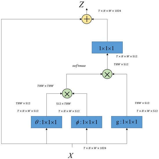
Figure 3.
Non-local block.
3.3. Multi-Scale Convolution
One simple observation is that a vehicle closer to the camera appears larger that one of the same actual size yet further from the camera. Put differently, the vehicle size on camera is not necessarily in proportion with its actual size. With our goal of estimating vehicle speed in mind, it is important to consider the differences of vehicle size on camera due to their different distances from the camera. Different distances from the camera give rise to different scales for vehicles, which makes determining the size of convolution kernel difficult. Our way of tackling this issue is to input the convolution kernels of different sizes to the first layers separately of the network, of which the outputs are concatenated to be the inputs of the next layer. The information with different scales is considered in multiple convolution kernels, making the network adaptive. Figure 4 shows our multi-scale CNN. The box on the left indicates the input of the model. The three boxes in the middle respectively represent the three different convolutional layers of convolutional kernels as , and . The large cuboid on the right represents that the resulting concatenated output, which is used as the input of the next layer.
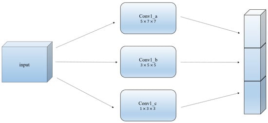
Figure 4.
Multi-scale CNN.
Figure 5 illustrates our final model. ‘Multi-scale conv’ refers to the multi-scale CNN we propose. On the basis of the IR(2+1)D50, we build non-local blocks into the second and third residual modules. The input of the model includes RGB images and optical flow images. In practice, the video stream can be directly decoded by OpenCV; the corresponding optical flow snippet can be extracted by the traditional optical flow algorithm or the deep learning method. Specifically, the optical flow used in this paper is obtained by dense optical flow [35]. After obtaining the RGB and optical flow frames, the data need to be standardized and resized to a fixed size. Finally, the RGB images and optical flow images can be stacked together as the input of the network.
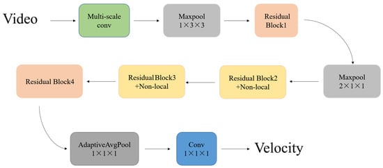
Figure 5.
Model Architecture.
4. Experiments and Analysis
In this section, we explain the experiments with variations of 3D ConvNets to estimate average vehicle speed in the video. The results are encouraging. In addition to variations of models, we comparatively experiment with different inputs. One notable finding is that the model result is sensitive to optical flow. To make the model more robust, we include non-local blocks and multi-scale convolution into IR(2+1)D model. Following is the details of the experiments. The code is in the supplementary material.
4.1. BrnoComSpeed Dataset
The dataset used is adapted from the BrnoCompSpeed Datase [23], which is a new benchmark dataset including 18 full-HD traffic monitoring videos. The traffic videos in this dataset were filmed in six different locations with three cameras (Panasonic HDC-SD90, Sony Handycam HDR-PJ410, Panasonic HC-X920) from different angles in each site. Each camera recorded an approximate a one hour-long video. The frame rate of the videos is 50 FPS, while the resolution is 1080p. The 20,865 vehicles recorded in the videos have been accurately annotated by LIDAR and verified by several reference GPS tracks. The videos in BrnoCompSpeed Dataset cover all typical traffic surveillance cameras angles and various traffic situations (small traffic flow in Session 3, large traffic flow in Sessions 5 and 6). Figure 6 is the sample images taken by six cameras in BrnoComSpeed Dataset. To show the environment clearly, we intentionally select the pictures with carless lanes.
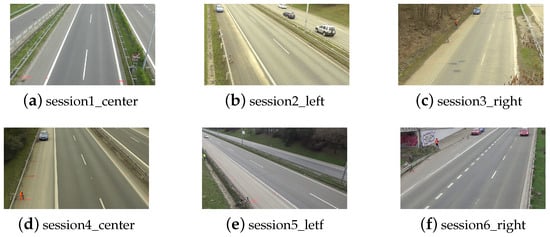
Figure 6.
Data sample.
Vehicle Speed Dataset: We split each of the 18 original videos from the BrnoCompSpeed Dataset into multiple short videos t seconds long each. Each t-second video clip is uesd as a sample. We then calculate the average vehicle speed in each of the t-second videos.Subsequently, we label each short video with the calculated average vehicle speed. The consideration behind splitting original videos is the tradeoff of time information length. It is understood that 3D ConvNets’ receptive field in time domain is limited, which means 3D ConvNets cannot process time information of a long length. On the other hand, too short videos are not sufficiently informative. On balance, we set in building the VehSpeedDataset10. Table 2 is on dataset partition over training and test sets. We distribute 80% of the total 5332 short videos to training set and the remaining 20% to test set.
Table 2.
Illustration of the Vehicle Speed Dataset named VehSpeedDataset10.
4.2. Implementation Details
We use AdamW [36] as the optimizer. We initialize the model parameters by inflating the 2D ImageNet pre-trained weights to 3D. The initial setting is as follows: learning rate ; weight decay in AdamW ; dropout ; training epoch 200. All experiments are implemented in Pytorch over 5-folds.
In the training phase, we estimate average vehicle speed in each short period based on the motion of the vehicle. Therefore, we select frame sequence at equal intervals from the video samples. This process is different from that in video action recognition, where successive frames are extracted from video footage. The input of 16 frames remains unchanged in the training and test phases.
Data Augmentation: It is acknowledged that data augmentation is of great importance in deep neural networks. Thus, we apply data augmentation in our model. In the training phase, we first resize a video image to and then randomly crop a patch from the image. We randomly choose the starting frame among video images with the consideration that the starting frame is sufficiently early so that a desired number of frames is guaranteed. The time intervals between frames, chosen as model inputs, are fixed and uniform. We also apply random left-right flipping for each video in the training phase. In the test phase, we resize an image to and then take the center patch.
4.3. 3D ConvNets and Non-Local Neural Networks
In this section, we compare the experimental performance across various 3D ConvNets on the dataset VehSpeedDataset10. The mean absolute error (MAE) and the mean squared error (MSE) are used as the model performance measures. Let denote a vector of predictions generated from a sample i including N data points and denote the corresponding vector of ground-truth in sample i. The MAE of the predictor is thus defined as:
And the MSE of the predictor is defined as:
4.3.1. Different 3D ConvNets
Table 3 comparatively displays the performance across various 3D ConvNets on VehSpeedDataset10. The model input is a sequence of RGB images. From the table, it can be seen that IR3D50 outperforms IR3D18 and IR3D34 in terms of MAE and MSE. In short, more layers in the 3D convolution network correspond to better results. These results are analogous to those in ImageNet [12].
Table 3.
The results of different 3D ConvNets on the VehSpeedDataset10.
For the 2D convolutional neural network, it is known that ResNet50 is better than Inception-V1 in the image classification problem. Nevertheless, we see from Table 3 that inception-v1 outperforms ResNet50 in the video-based speed estimation problem. One explanation is that 3D ConvNets are much more complicated than 2D ConvNets and the 2D ConvNets convolution is inadequate for 3D ConvNets.
Another inspection from the Table 3 is IR(2+1)D50 shows the best performance on the test set. The MAE of IR(2+1)D50 is lower than that of IR3D50, while the MSE lower. This striking comparison suggests that in the video-based vehicle speed estimation problem, the results can significantly improve with spatial and temporal dimensions considered separately in a 3D convolution. The rationale is that spatial domain and time domain are not symmetrical. Thus, the features in image sequences are better captured with the two domains considered separately. Furthermore, 3D ConvNets are significantly more complicated than 2D, which necessitates appropriate modifications in converting the 2D network structure to the 3D counterpart.
4.3.2. Adding Optical Flow Information
Optical flow is the observed motion pattern of objects, surfaces, and edges in a visual scene caused by relative motion between an observer and a scene [37,38]. It can also be defined as apparent velocity of brightness patterns in an image. As optical flow reflects the velocity of pixel points, and the velocity of a vehicle is closely related to that of all the pixel points comprising the vehicle, optical flow information is a logical and useful additional input to our model.
As show in Table 4, we experiment with various input resolutions of , , on IR(2+1)D50, corresponding to the original video frames resized to , , , respectively. Because the last pooling layer is Adaptive Pooling, the network produces the same sized output for different input sizes. From Table 4, we inspect that input size of gives the highest MAE and MSE. That is because resizing images too small causes a loss of useful information. As the input size grows, the information in input accordingly increases. So that error measure consistently decreases as the input size increases. However, increase in input size also brings redundant information, which causes increase in error measures. Thus, the marginal improvement diminishes as the input size increases due to this tradeoff.
Table 4.
Influence of different input on the IR(2+1)D50.
Experimental results in Table 4 suggest that input size and form have a significant impact on the performance of the model. Here, “cat” means that RGB images and optical flow images are concatenated together as input. Table 4 shows the model results for three input forms in three rows. More specifically, the first row corresponds to the RGB images sequence used as the input; the second corresponds to optical flow images as the input; the third corresponds to “cat” as input. It can be seen that optical flow input gives significantly better results than that of RGB input, everything else equal. Clearly, optical flow information is more suitable an input form for our model in vehicle speed estimation problem. One explanation for this observation is since optical flow reflects the motion of pixel points, it incorporates more useful vehicle speed information.
An interesting observation is that in the video action classification problem, RGB input outperforms optical flow [14]. In contrast, the results are reverse in the vehicle speed estimation problem. Problems differ in terms of structure. It is crucial to propose a fitting solution supported by a deep understanding and consideration of the particular structure of the problem of interest.
4.3.3. Non-Local Blocks and Multi-Scale
It is known that the convolutional neural network is mainly concerned with local information. However, the vehicle speed estimation problem requires consideration of the vehicle trajectory change throughout the entire video footage. In order to focus on more global information, we add non-local blocks to the second and third residual blocks of the network. Besides, we add a convolutional layer whose kernel is (3, 5, 5), the stride is (1, 2, 2) after the first convolutional layer to reduce video memory. Moreover, we also change the first layer of the ConvNet to the multi-scale convolution detailed in Section 3.3.
Comparative experimental results across model configurations are presented in Table 5. To facilitate understanding, we adopt straightforward naming conventions, e.g., ’conv_add’ indicates the convolutional layer with the convolution kernel size of and the stride size of , which are added after the first layer. The numerical results are shown in Table 6.
Table 5.
Different configurations of models.
Table 6.
Influence of non-local blocks and multi-scale convolution.
From Table 6, it can be seen that the additional layer of convolution in the network does not reduce the useful information and model performance does not degrade with the addition of the convolutional layer. The incorporation of non-local blocks into the IR(2+1)D model leads to improved model results, suggesting that non-local and 3D ConvNets are complementary, which can be understood that 3D ConvNets capture local features and the additional non-local blocks shed light on global information. Additionally, the model performance further improves with multi-scale convolution being used. The reason is that multi-scale convolution can increase the richness and diversity of features, thus better capture different sizes of vehicle motion information in the video.
4.3.4. Comparison of Different Methods
Table 7 shows the comparative experimental results of our method and other methods. Among the other methods, OPtCalib, OPtCalibVP2, OPtScale, OPtScaleVP2 are presented in [23] and the scale is computed as the mean of scale values obtained from the distance measurements on the road.
Table 7.
Comparison of different Methods on the same dataset.
It can be seen from the table our method underperforms OptScale, OptCalib, and OptCalibVP2. The main reason is the different error measure calculation. There are two sources of error to the camera calibration-based methods: (1) the error from camera calibration; (2) the error from detection and tracking. The error calculation of camera calibration-based methods presented here only contains the first error source, i.e., the error from camera calibration, whereas does not take account of the second error source, i.e., the detection and tracking cause error.
However, the detection and tracking caused errors are not negligible. Since the speed calculation by camera calibration-based methods heavily relies on the results from the detection and tracking, an error in detection or tracking can greatly distort the vehicle trajectory, which in turn will lead to significantly off speed or even make the speed calculation undoable. It is clear that the errors that arise in detection and tracking will be carried on and compounded in the subsequent calculations. Besides, detection and tracking are prone to errors. In practice, a variety of common suboptimal environments (illumination variation, motion blur, background clutter and overlapping, etc.) could cause errors in the detection and tracking phases, including detection missing, false detection, tracking loss, etc. Considering the prevalence and significance of the detection and tracking errors, it is believed that the error results of the calibration-based methods would be profoundly greater with the neglected detection and tracking errors included. In contrast, our methods do not utilize detection and tracking, which means there are no the detection and tracking errors. Therefore, if detection and tracking-included error is taken into consideration, the error measure of the calibration-based methods would be higher than that of our methods.
Our deep learning-based method to the average vehicle speed estimation problem heavily relies on data. In other words, a large quantity of labeled data needs to be accessible for the method to be effective. With extensive high quality data in place, our method is effective regardless of the environmental and weather conditions. In other words, our method is a self-closed end-to-end framework, which does not need manual intervention and does not rely on any other external factors nor subprocesses such as detection and tracking. However, there is an appreciable gap between the error measure of our method and that of GPS and RADAR.
5. Conclusions and Future Work
This paper proposes a deep learning-based method to the average vehicle speed estimation problem. This method has a desirable feature of not requiring manual intervention. Compared with other common vehicle estimation methods, the proposed method is not dependent on external environment factors, nor does it on vehicle detection and tracking processes. In summary, it is a self-closed end-to-end framework.
Based on ResNet50, we propose an end-to-end IR(2+1)D50-cNLms model to estimate average vehicle speed based on video footage. The modified method IR(2+1)D50-cNLms has a global spatial-temporal perspective on the information in the video. We experiment with different 3D ConvNets on VehSpeedDataset10. The experiments suggest that optical flow is crucial information for the vehicle speed estimation problem. By using both RGB images and optical flow as inputs, our IR(2+1)D50-cNLms model performs exceedingly well.
A limitation on our model is lack of quality data. As noted previously, deep learning-based models require extensive labeled data, which is lacking. The lack of data could lead to 3D ConvNets overfitting. In the future, we can try to expand our dataset to improve the model performance. Inspired by [39] using multi-sensor data fusion to construct the model, we can also try to integrate RGB images and optical flow for more effective features extraction with the understanding of the marked differences between the two input types.
Supplementary Materials
The following are available online at https://www.mdpi.com/1999-5903/11/6/123/s1. This is the code for the models we built in this article.
Author Contributions
Conceptualization, Z.Y.; methodology, H.D.; software, H.D. and M.W.; validation, H.D., M.W. and Z.Y.; formal analysis, H.D.; investigation, H.D.; resources, Z.Y.; data curation, H.D.; writing—original draft preparation, H.D.; writing—review and editing, H.D., M.W. and Z.Y.; visualization, H.D. and M.W.; supervision, Z.Y.; project administration, Z.Y.
Funding
This research received no external funding.
Conflicts of Interest
The authors declare no conflict of interest.
Abbreviations
The following abbreviations are used in this manuscript:
| 3D ConvNets | 3-dimensional convolutional networks |
| MAE | Mean absolute error |
| MSE | Mean square error |
| RoI | Region of Interest |
References
- Lan, J.; Li, J.; Hu, G.; Ran, B.; Wang, L. Vehicle speed measurement based on gray constraint optical flow algorithm. Optik-Int. J. Light Electron Opt. 2014, 125, 289–295. [Google Scholar] [CrossRef]
- Mathew, T. Intrusive and Non-Intrusive Technologies; Tech. Rep; Indian Institute of Technology Bombay: Mumbai, India, 2014. [Google Scholar]
- Luvizon, D.C.; Nassu, B.T.; Minetto, R. A video-based system for vehicle speed measurement in urban roadways. IEEE Trans. Intell. Transp. Syst. 2017, 18, 1393–1404. [Google Scholar] [CrossRef]
- Huang, T. Traffic speed estimation from surveillance video data. In Proceedings of the IEEE Conference on Computer Vision and Pattern Recognition Workshops, Salt Lake City, UT, USA, 18–22 June 2018; pp. 161–165. [Google Scholar]
- Nurhadiyatna, A.; Hardjono, B.; Wibisono, A.; Sina, I.; Jatmiko, W.; Ma’sum, M.A.; Mursanto, P. Improved vehicle speed estimation using gaussian mixture model and hole filling algorithm. In Proceedings of the 2013 International Conference on Advanced Computer Science and Information Systems (ICACSIS), Bali, Indonesia, 28–29 September 2013; pp. 451–456. [Google Scholar]
- Wang, H.; Liu, L.; Dong, S.; Qian, Z.; Wei, H. A novel work zone short-term vehicle-type specific traffic speed prediction model through the hybrid EMD–ARIMA framework. Transportmet. B Transp. Dyn. 2016, 4, 159–186. [Google Scholar] [CrossRef]
- Maduro, C.; Batista, K.; Peixoto, P.; Batista, J. Estimation of vehicle velocity and traffic intensity using rectified images. In Proceedings of the 2008 15th IEEE International Conference on Image Processing, San Diego, CA, USA, 12—15 October 2008; pp. 777–780. [Google Scholar]
- Sina, I.; Wibisono, A.; Nurhadiyatna, A.; Hardjono, B.; Jatmiko, W.; Mursanto, P. Vehicle counting and speed measurement using headlight detection. In Proceedings of the 2013 International Conference on Advanced Computer Science and Information Systems (ICACSIS), Bali, Indonesia, 28–29 September 2013; pp. 149–154. [Google Scholar]
- Dailey, D.J.; Cathey, F.W.; Pumrin, S. An algorithm to estimate mean traffic speed using uncalibrated cameras. IEEE Trans. Intell. Transp. Syst. 2000, 1, 98–107. [Google Scholar] [CrossRef]
- Grammatikopoulos, L.; Karras, G. Automatic estimation of vehicle speed from uncalibrated video sequences. In Proceedings of the FIG-ISPRS-ICA International Symposium on Modern Technologies, Education & Professional Practice in Geodesy & Related Fields, Sofia, Bulgaria, 9–10 November 2006. [Google Scholar]
- Nam, H.; Baek, M.; Han, B. Modeling and propagating cnns in a tree structure for visual tracking. arXiv 2016, arXiv:1608.07242. [Google Scholar]
- He, K.; Zhang, X.; Ren, S.; Sun, J. Deep residual learning for image recognition. In Proceedings of the IEEE Conference on Computer Vision and Pattern Recognition, Las Vegas, NV, USA, 26 June–1 July 2016; pp. 770–778. [Google Scholar]
- Lin, T.Y.; Dollár, P.; Girshick, R.B.; He, K.; Hariharan, B.; Belongie, S.J. Feature Pyramid Networks for Object Detection. In Proceedings of the IEEE Conference on Computer Vision and Pattern Recognition, Honolulu, HI, USA, 21–26 July 2017; Volume 1, p. 4. [Google Scholar]
- Carreira, J.; Zisserman, A. Quo vadis, action recognition? A new model and the kinetics dataset. In Proceedings of the IEEE Conference on Computer Vision and Pattern Recognition, Honolulu, HI, USA, 21–26 July 2017; pp. 4724–4733. [Google Scholar]
- He, X.C.; Yung, N.H. A novel algorithm for estimating vehicle speed from two consecutive images. In Proceedings of the 2007 IEEE Workshop on Applications of Computer Vision (WACV ’07), Austin, TX, USA, 21–22 February 2007; p. 12. [Google Scholar]
- You, X.; Zheng, Y. An accurate and practical calibration method for roadside camera using two vanishing points. Neurocomputing 2016, 204, 222–230. [Google Scholar] [CrossRef]
- He, X.; Yung, N.H.C. New method for overcoming ill-conditioning in vanishing-point-based camera calibration. Opt. Eng. 2007, 46, 037202. [Google Scholar] [CrossRef]
- Kumar, A.; Khorramshahi, P.; Lin, W.A.; Dhar, P.; Chen, J.C.; Chellappa, R. A semi-automatic 2D solution for vehicle speed estimation from monocular videos. In Proceedings of the IEEE Conference on Computer Vision and Pattern Recognition (CVPR) Workshops 2018, Salt Lake City, UT, USA, 18–22 June 2018. [Google Scholar]
- Wojke, N.; Bewley, A.; Paulus, D. Simple online and realtime tracking with a deep association metric. In Proceedings of the 2017 IEEE International Conference on Image Processing (ICIP), Beijing, China, 17–20 September 2017; pp. 3645–3649. [Google Scholar]
- Dubská, M.; Herout, A.; Sochor, J. Automatic Camera Calibration for Traffic Understanding. BMVC 2014, 4, 8. [Google Scholar]
- Sochor, J.; Juránek, R.; Herout, A. Traffic surveillance camera calibration by 3d model bounding box alignment for accurate vehicle speed measurement. Comput. Vis. Image Underst. 2017, 161, 87–98. [Google Scholar] [CrossRef]
- Filipiak, P.; Golenko, B.; Dolega, C. NSGA-II Based Auto-Calibration of Automatic Number Plate Recognition Camera for Vehicle Speed Measurement. In Proceedings of the European Conference on the Applications of Evolutionary Computation, Porto, Portugal, 30 March–1 April 2016; pp. 803–818. [Google Scholar]
- Sochor, J.; Juránek, R.; Špaňhel, J.; Maršík, L.; Širokỳ, A.; Herout, A.; Zemčík, P. Comprehensive Data Set for Automatic Single Camera Visual Speed Measurement. IEEE Trans. Intell. Transp. Syst. 2018, 20, 1633–1643. [Google Scholar] [CrossRef]
- Ji, S.; Xu, W.; Yang, M.; Yu, K. 3D convolutional neural networks for human action recognition. IEEE Trans. Pattern Anal. Mach. Intell. 2013, 35, 221–231. [Google Scholar] [CrossRef] [PubMed]
- Tran, D.; Bourdev, L.; Fergus, R.; Torresani, L.; Paluri, M. Learning spatiotemporal features with 3d convolutional networks. In Proceedings of the IEEE International Conference on Computer Vision (ICCV), Santiago, Chile, 11–18 December 2015; pp. 4489–4497. [Google Scholar]
- Feichtenhofer, C.; Pinz, A.; Wildes, R. Spatiotemporal residual networks for video action recognition. In Proceedings of the Advances in Neural Information Processing Systems, Barcelona, Spain, 5–10 December 2016; pp. 3468–3476. [Google Scholar]
- Simonyan, K.; Zisserman, A. Two-stream convolutional networks for action recognition in videos. In Proceedings of the Advances in Neural Information Processing Systems, Montreal, QC, Canada, 8–13 December 2014; pp. 568–576. [Google Scholar]
- Tran, D.; Ray, J.; Shou, Z.; Chang, S.F.; Paluri, M. Convnet architecture search for spatiotemporal feature learning. arXiv 2017, arXiv:1708.05038. [Google Scholar]
- Qiu, Z.; Yao, T.; Mei, T. Learning spatio-temporal representation with pseudo-3d residual networks. In Proceedings of the IEEE International Conference on Computer Vision (ICCV), Venice, Italy, 22–29 October 2017; pp. 5534–5542. [Google Scholar]
- Tran, D.; Wang, H.; Torresani, L.; Ray, J.; LeCun, Y.; Paluri, M. A Closer Look at Spatiotemporal Convolutions for Action Recognition. In Proceedings of the IEEE Conference on Computer Vision and Pattern Recognition (CVPR) Workshops 2018, Salt Lake City, UT, USA, 18–22 June 2018; pp. 6450–6459. [Google Scholar]
- Buades, A.; Coll, B.; Morel, J.M. A non-local algorithm for image denoising. In Proceedings of the 2005 IEEE Computer Society Conference on Computer Vision and Pattern Recognition (CVPR’05), San Diego, CA, USA, 20–26 June 2005; Volume 2, pp. 60–65. [Google Scholar]
- Dabov, K.; Foi, A.; Katkovnik, V.; Egiazarian, K. Image denoising by sparse 3-D transform-domain collaborative filtering. IEEE Trans. Image Proc. 2007, 16, 2080–2095. [Google Scholar] [CrossRef]
- Wang, X.; Girshick, R.; Gupta, A.; He, K. Non-local neural networks. arXiv 2017, arXiv:1711.07971. [Google Scholar]
- Vaswani, A.; Shazeer, N.; Parmar, N.; Uszkoreit, J.; Jones, L.; Gomez, A.N.; Kaiser, Ł.; Polosukhin, I. Attention is all you need. In Proceedings of the Advances in Neural Information Processing Systems, Long Beach, CA, USA, 4–9 December 2017; pp. 5998–6008. [Google Scholar]
- Farnebäck, G. Two-frame motion estimation based on polynomial expansion. In Proceedings of the Scandinavian Conference on Image Analysis, Halmstad, Sweden, 29 June–2 July 2003; pp. 363–370. [Google Scholar]
- Loshchilov, I.; Hutter, F. Fixing weight decay regularization in adam. arXiv 2017, arXiv:1711.05101. [Google Scholar]
- Burton, A.; Radford, J. Thinking in Perspective: Critical Essays in the Study of Thought Processes; Routledge: Abingdon, UK, 1978; Volume 646. [Google Scholar]
- Warren, D.H.; Strelow, E.R. Electronic Spatial Sensing for the Blind: Contributions from Perception, Rehabilitation, and Computer Vision; Springer Science & Business Media: Berlin/Heidelberg, Germany, 2013; Volume 99. [Google Scholar]
- Rodger, J.A. Toward reducing failure risk in an integrated vehicle health maintenance system: A fuzzy multi-sensor data fusion Kalman filter approach for IVHMS. Exp. Syst. Appl. 2012, 39, 9821–9836. [Google Scholar] [CrossRef]
© 2019 by the authors. Licensee MDPI, Basel, Switzerland. This article is an open access article distributed under the terms and conditions of the Creative Commons Attribution (CC BY) license (http://creativecommons.org/licenses/by/4.0/).