1. Introduction
Overcrowding of hospital waiting rooms by patients characterizes the outpatient departments (OPDs) of healthcare centers of developing countries [
1,
2]. It is true that most of the patients that visit health centers have varying health challenges and some may require prompt medical attention. However, due to overcrowding, these patients are made to endure a lengthy and painful wait for treatment [
3,
4]. In the developing world, the problem is aggravated by the fact that health facilities are few, scattered and under-staffed. In such countries, it is a common experience for patients visiting an OPD to return home without receiving medical attention. For example, data collected from the patients record book at one general OPD showed that, within a one month period, of the 2211 patients who walked-in into the OPD department, only 1870
patients were seen and 341
patients were not seen [
5].
To deal with such excess demand, physicians may opt to work overtime or delegate some work to nurses. Consequently, this may cause the healthcare center to incur extra costs and/or provide reduced quality of service to the patients [
6,
7]. Reduced quality of service might impact patient’s trust in the health facility and/or practitioners [
8]. Overcrowding in hospitals also relates to patients’ safety. Due to limited space, patients may be placed in inappropriate spaces, which can be a recipe for complications and fatalities. The challenge further result from the fact that, in the developing world, patients’ hospital visits (especially to the OPD) are rarely scheduled, which makes it difficult to project daily demand for the services [
9,
10]. This leads to an inbalance between hospital staffing ratios and health service demand. It is the case in many situations that as one heath center is being pressed with high demand beyond its capacity, the facilities nearby may have few patients. However, there is no mechanism for a timely exchange of information about patient load between health facilities. This leads to patients in overcrowded health facilities having to endure a lengthy and painful wait for treatment which may not even be given.
Patients are usually transferred between health facilities and the purpose for such transfers is to maintain the continuity of medical care. Normally, these are patients that require specialized treatment or procedures and are transferred to facilities with such specialized equipment and personnel, i.e., the benefits of care available at another facility against the potential risks involved. The patient transfer process involves such key elements as the decision to transfer and notification, patient pre-transfer stabilization and preparation, the choice of appropriate mode of transfer (e.g., land or air transport), personnel to accompany the patient, equipment and monitoring required during the transfer and finally the documentation and handover of the patient at the receiving facility [
11,
12]. In each transfer these key elements are followed so as not to affect patient prognosis.
Since our focus is the outpatient department, we make the following assumptions: (1) Upon arrival, patients are triaged such that the critical patients are served first and then the least critical last. (2) Excess patient loads can only be transferred once, i.e., a patient can only be transferred once. As pointed out above, the patient transfer process starts with a decision to transfer the patient because of the exposure of the patient and the staff to additional risks and additional expenses for the guardians. A senior consultant level doctor is responsible for making the decision to transfer the patient . A patient’s guardians are made aware of the benefits and risks involved during such a transfer. Written and informed consent of patients’ relatives along with the reason(s) to transfer is mandatory before the transfer. In this work, the role of the senior doctor will be played by the central controller of the system. Since the system provides the patient with alternative healthcare service sources, it is up to the patient to go to the recommended facility or wait in the queue and risk returning home without getting medical care. Hence a patient’s consent will be by virtually in accepting to go to the recommended facility. Since patients are triaged upon arrival (with the most critical served first), we assume that the patients being recommended for transfer are stable enough such that pre-transfer stabilization and preparation are not required. The choice of an appropriate mode of transport is key in this work and is covered in
Section 6. The consideration of guardian, patient monitoring during transfer and documentation are beyond the scope of this work.
By intelligently re-assigning patients from congested facilities to less congested ones, overcrowding of OPDs can be managed in a timely way. Re-assigning excess patient loads reduces the number of patients that return to their homes without being attended to by physicians and consequently leads to improvement of the quality of the service demanded of medical staff being kept to a minimum. Patient flows in hospitals are usually not continuous and stable; rather, patient flows are complex and may change suddenly [
13]. Hospitals experience two kinds of service demands: (1) Event driven demand, i.e., ambulatory arrivals during accidents and natural disasters, and (2) regular demand from the catchment area. However, a lack of real time patient flow information may result in some health facilities straining to satisfy the demand while at the same time facilities in the same vicinity may have minimal demand. While patients may be wary about being transferred to a hospital they know little or nothing about, such transfers may significantly reduce the amount of time a patient must wait to get medical care [
14]. Attempts in the literature exist to predict patient traffic, but most of the work focuses on patient flow in the emergency department (ED) [
15,
16]. Furthermore, independent attempts have been made to predict and schedule traffic flow [
17,
18]. However, to our knowledge, no literature has explored the integration of the two processes using machine learning techniques.
In this paper, a deep learning-based patient load prediction model is proposed. The model aides in overcoming the effects of overcrowding in hospital waiting rooms, which results from a mismatch between hospital staffing ratios and the demand for healthcare services. Overcrowding of hospital waiting rooms leads to excessive patient waiting times, incomplete service delivery and unhappy medical staff. Worse, due to the limited patient loads that a health facility can handle, patients may leave the facility before the medical examination is complete. However, it is true that, as one health facility may be struggling with excessive patient load, another facility in the vicinity may have low patient turn out. In this work, we assume the existence of a hospital information management system, which enables timely sharing of excess patient load information among hospitals [
19]. The proposed machine learning-based patient load prediction model takes current and historical patient load data as inputs and outputs future predicted patient load. Furthermore, in the case of excess patient loads, we propose to re-assign excess loads to nearby facilities that have a minimal load as a way to control overcrowding and reduce the number of patients that leave health facilities without receiving medical care.
The re-assigning of patients will imply a need for transportation for the patient to move from one facility to another. To avoid putting a further strain on the already fragmented ambulatory services, we assume the existence of a scheduled bus transport system which can support the timely movement of patients from the bus stop nearest to the source facility to the destination facility. Building on this assumption we propose an Internet of Things (IoT) integrated smart bus system. We develop an Arduino-based smart bus system that can be tagged on public buses and can be queried by patients through representation state transfer application program interfaces (APIs) to provide them with the position of the buses through web app or SMS relative to their origin and destination stop. The back end of the proposed system is based on message queue telemetry transport (MQTT), which is lightweight, data efficient and scalable, unlike the traditionally used hypertext transfer protocol (HTTP). To ensure the reliability of the smart transport system, our solution makes use of the real time location of the buses to compute the approximated time for the bus to reach a particular destination. By saving a bus’s location data on the server together with corresponding timestamps, the system is able to estimate the arrival time of the bus to a particular bus stop. Alternatively, the arrival time can also be approximated using services like Google maps [
20].
The Internet of Things (IoT) enables advanced services by interconnecting physical and virtual things based on existing and evolving inter-operable information and communication technologies. The IoT gives immediate access to information about physical objects and leads to innovative services with high efficiency and productivity [
21]. Building on the power of IoT, we demonstrate its application in the transportation system by developing an IoT-based smart bus system. Generally, a smart bus system consist of four basic components, namely smart bus depots, smart bus stops, smart buses and interactive citizen interfaces (web portal based and smart phone app based). Each of these components are connected through the Internet. The smart bus depots, smart bus stops and smart buses consist of a number of heterogeneous wireless and embedded sensors. These sensor networks are connected to the city internet backbone through Wi-Fi hotspots in the bus stops, depots and inside buses. These intelligent autonomous devices attached to or embedded into the system senses the user requirements and interacts with them, shares information with other devices and takes decisions without any human intervention. Buses are widely used public transportation in many cities today. Normal buses can be converted into smart buses with the incorporation of intelligent sensors and IoT devices. Our contributions in this paper are three fold:
Using a deep learning approach, we predict patient traffic flow.
We combine the deep learning patient load prediction and hospital assignment using the predicted patient load as criterion to perform the intelligent hospital assignment.
We develop an IoT-based smart bus system. We explore scalable and efficient techniques that allow the system to handle increased requests for data.
The remainder of this paper is organized as follows. In
Section 2, a review of the relevant literature and machine learning structures is presented. In
Section 3, we model our system architecture and training model. In
Section 4, we propose a deep learning-based patient load prediction method. In
Section 6, we present our proposed IoT-based smart bus system that allows the estimation of the time for the smart bus to arrive at a bus stop, or the time for it to reach a destination such that transferred patients do not experience unnecessary delays due to transport congestion. Finally,
Section 7 concludes the paper.
2. Related Work
A lot of research efforts have been made to deal with the problem of overcrowding with regard to the ED of the hospital [
22,
23,
24,
25]. To deal with this problem, inter-hospital transfers have been proposed as a possible solution [
26]. However, overcrowding is also a problem in the OPD and equally affects patient satisfaction, which is affected by the efficiency of the services rendered. Efficient provision of health services encompasses such issues as waiting time to consultation, duration of consultation, timely response to emergencies, quick drug dispensation, and timely and accurate diagnosis [
27,
28]. The challenge in dealing with excess demand results from the challenges in predicting patient flow in the OPD. Patient load forecasting involves predicting patient loads for future time periods. Depending on time horizons, patient load prediction can be categorized into: Long-range forecasting, medium-range forecasting, short-range forecasting and real-time or very short-term forecasting. Accurate patient flow predictions may aide in improving hospital management efficiency.
Traditional methods have been applied in forecasting hospital visits. In [
29], Dan and Qualls explored the problem of predicting ED patient volume, length of stay and acuity. They studied five models, namely raw observations, moving averages, mean values with moving averages, seasonal indicators with moving averages and auto-regressive integrated moving averages (ARIMAs). It was discovered in this study that simpler models performed best. In [
30], Rotstein et al. explore the problem of short-range forecasting of patient volume. A general linear model (GLM) is formulated that can be applied for short-range forecasting of patient volume. In [
31], Batal et al. developed equations for predicting daily patient volumes via stepwise linear regression analysis. In [
32], Reis and Mandl developed a trimmed mean seasonal model for the expected number of daily patient visits to an ED. In [
33], Brillman et al. constructed a first order cyclical regression model with fixed-width sine and cosine harmonics as the seasonal component and a hierarchical model with a scalable Gaussian function as the seasonal component for ED daily respiratory chief complaints. In [
34], Flottemesch et al. formulated a mathematical model for forecasting ED censuses. In [
35], Boyle et al. investigated the performance of a general linear regression model formed with 11 dummy variables in forecasting monthly patient admissions. In [
36], Au-Yeung et al. forecasted patient arrivals to an accident and ED via a structural time series model. In [
37], Kam et al. studied the problem of predicting daily patient numbers for a regional medical center via the application of time series analysis. Capan et al. applied time series analyses; specifically, they applied best-fitting models of ARIMA and linear regression to various prediction models and compared the results using error statistics. Their work aimed at forecasting censuses in neonatal intensive care units (NICU) [
38]. Other interesting studies relating to predicting patient flow in ED have been reported in [
39,
40,
41,
42]. While these traditional techniques are popular in forecasting hospital visits, they are not good at dealing with complexity in hospital visits data.
Artificial Intelligence techniques, e.g., artificial neural networks (ANNs), form another approach for hospital visit forecasting [
43]. However, ANN is not as prevalent as the traditional methods in this field. In [
44], Jones et al. explored the performance comparison of exponential smoothing, seasonal ARIMA, ANN and time series regression in daily ED patient volume prediction with linear regression. Their results show that the former four methods did not perform consistently in forecasting with a sample, although they all performed better in sample fitting. In [
45], Aladag and Aladag modeled the number of outpatient visits by ANN using different activation functions. In [
46], Xu et al. modeled daily patient arrivals at ED via ANN. Kottalanka et al. developed an artificial intelligence model based on back-propagation Neural Network for predicting patient inflow [
47]. Clearly, more research is needed to demonstrate and harness the power of machine learning to improve the provision of healthy services, which can lead to improved quality of care and also efficient utilization of resources.
The patient flow data is basically time series data. In [
48], a time series is defined as a vector
, where each element
pertaining to
X is an array of
m values
, with each of the
m values corresponding to the input variables measured in the time series. Several traditional techniques of manipulating time series data including traditional ANNs have been exploited in the literature for applications in economics, engineering and medicine [
49,
50]. Deep learning, however, has shown an exceptional performance in both classification and forecasting applications [
51,
52,
53]. For classification, the existing methods generally relied on the usage of domain specific features normally crafted manually by human experts. However, getting best features was a daunting task and the performance of the classifier was heavily dependent on their quality. The advantage of deep learning is in its ability to learn such features by itself, reducing the need for human experts [
54,
55].
Convolutional neural network (CNN) models have continued to gain popularity among the deep learning community in various domains [
56]. Due to their efficiency with data that has a topological structure in the features space, CNN models have achieved the best results in computer vision [
57]. They have also been applied successfully to sequential data such as sentences, time series and speech [
58,
59,
60,
61,
62,
63]. CNNs employ sets of shared weights across the whole input, which is efficient both statistically and computationally. CNNs are particularly interesting in domains associated with the processing of large amounts of data [
64]. Since patient load data and traffic data can be categorized as big data, the application of deep learning-based solutions is suited to solve the combined problem of patient load predictions and intelligent inter-hospital patient transfers.
We point out that in recent times deep reinforcement learning (Deep-RL) has gained popularity. Deep learning basically models a scenario in which no direct interaction exist between the algorithm and the environment it is operating in. Basically, RL enables a feedback loop between the algorithm and the environment. It allows the algorithm to experience a dataset that varies with time as a result of the interaction with the surrounding environment. RL is applicable to scenarios that can be modeled by a Markov decision process (MDP). Recent works based on RL techniques have shown comparable performance against NNs. In [
65], Negnevitsky et al. applied an adaptive neural fuzzy inference system (ANFIS) to study the problem of load forecasting in power systems. They further pointed out the difficulty of load forecasting in power systems resulting from the complexity of the power load series as it exhibits seasonality levels and the fact that power load series have various weather related exogenous variables. In [
66], the authors applied principles of RL and game theory to develop an autonomous evacuation process to support distributed and efficient evacuation planning. Deep-RL methods results when deep NNs are used to approximate any of the components of RL, e.g., action-value and/or the policy functions [
67]. A combination of NN with RL will enable solving even more complex problems.
Despite the wide range of successes, current state-of-the-art Deep-RL methods still face a number of significant drawbacks [
68]. As the training of NNs requires huge amounts of data, Deep-RL demonstrates unsatisfying results in settings where data generation is expensive. Even in cases where interaction is nearly free (e.g., in simulated environments), Deep-RL algorithms tend to require excessive amounts of iterations, which raises their computational and wall-clock time cost. Furthermore, Deep-RL suffers from random initialization and hyperparameter sensitivity, and its optimization process is known to be uncomfortably unstable [
69]. An especially embarrassing consequence of these Deep-RL features turned out to be the low reproducibility of empirical observations from different research groups [
70]. The main reason for NN becoming so popular lies in its ability to learn complex and nonlinear relationships that are difficult to model with conventional techniques [
71,
72]. Hence our choice of deep learning is based on its many documented exciting achievements [
73,
74], which are a function of big data, powerful computation, new algorithmic techniques, mature software packages and architectures and strong financial support.
Deep Learning Architectures
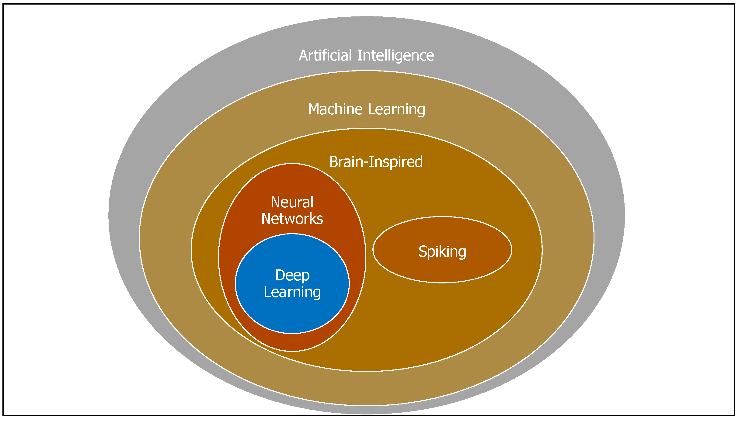
Deep NNs are a part of the broad field of AI. AI is the science and engineering of creating intelligent machines that have the ability to achieve goals like humans do.
Figure 1 shows the relationship of deep learning to the entire field of AI [
75]. There exist different deep learning structures including the deep Boltzmann machines (DBMs) and deep convolutional neural networks (CNNs). These architectures can be modeled to help control patient flow systems. The chosen deep belief architecture (DBA) has
L layers, including one input layer, one visible output layer and
hidden layers. The units comprising each layer except for the input layer have their own weight value called bias. The units for two adjacent layers are connected with each other via weighted links, while no inner layer connection exists.
3. System Modeling
In this section we describe our system architecture and the training process. We start by presenting the notations used through out the remainder of this paper in
Table 1.
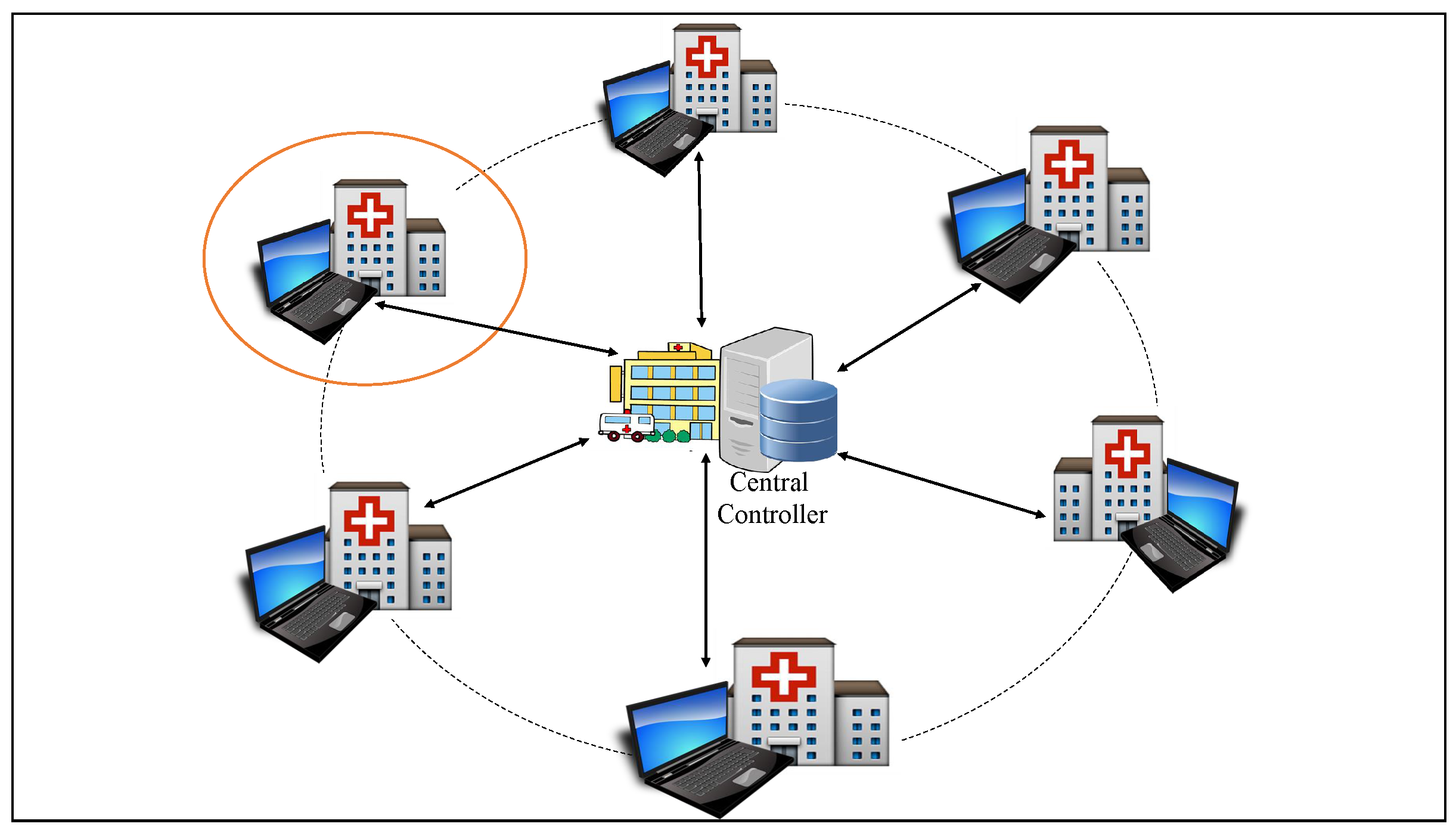
We model the system as a graph , where:
C is the central controller. The central controller can be played by the big health facility within a defined catchment area.
is the set of local hospitals under the control of C.
Given that M is the number of hospitals under consideration, we define the following;
Let
be the number of patients at the
mth hospital at time
t. Then:
is the set of patients over the set of hospitals at time
t.
Note that, here, M is the total number of hospitals located in a particular region with each hospital serving a population in its catchment area. If we let R be the average number of patients in the catchment area of L, i.e., the total catchment area covering the M hospitals, then . R is also time variant, since the population of a particular area varies with time. Each local hospital maintains a local database of patient information.
Define
E to represent the edges in a graph
G. Let an edge
in the graph represent the route connecting the two nearest hospitals. Then the weight,
, represents the obstacles that will impact a patient’s ability to get from one facility to another. These obstacles include distance, traffic congestion, transport cost and the physical terrain. Here we consider the shortest possible road connecting two facilities. In
Figure 2, the arrows indicate information flow between the central controller and each of the facilities in its domain and the solid circular line defines a catchment area while the dotted circular line defines a network of health facilities under the control of the central controller. From now on we abbreviate central controller as Cc.
Training the Model
Let the pair
represent the values of units in the input and output layers, respectively. Let
represent the weight of the link between units
i and
j, and
represent the bias of unit
i. Let
w be the matrix of the weights of all links and
b be the matrix of all the bias values; then the training of the deep belief architecture (DBA) comprises two steps, namely forward propagation and back propagation processes. Here, forward propagation is used for constructing the structure and activating the output, whilst back propagation is used for adapting the structure and fine-tuning the values of the weight and bias matrices. The forward propagation process can be modeled as a log-likelihood function and is given as:
where
denotes the
tth training data. Here, the DBA training can be seen as a log-linear Markov random field (MRF). As such,
represents the probability of
.
m is the total amount of training data.
The purpose of the training process is to minimize
, in the back propagation process. Back propagation is an efficient way to compute the partial derivatives of the gradient. It is a computation derived from the chain rule of calculus, and it operates by passing values backwards through the network to compute how the loss is affected by each weight. The link weight
w and the bias
b are adjusted using the gradient descent method. We represent
w and
b as:
where
is the learning rate of the training process. The Gradient descent is a first-order optimization method, this means it uses only information of the first derivative of the error; hence, it can be used in combination with error back propagation. The challenge with this method is the difficulty of choosing the learning rate so as to get fast learning but at the same time avoid oscillation.
As the input layer increases (i.e., gets larger) and becomes less connected in high dimensions, the DBA structure becomes inefficient as it fails to capture the spatial features efficiently. The CNNs tend to be powerful in this regard. The convolution operation extracts features of the input, and the parameters of the convolution operation comprise a set of learnable filters. Let
denote the filters and the
kth filter be represented by
, then the convolution operation outputs a feature map given as:
where
is the activation function and
is the activated value of the unit in the
ith row and
jth column of the feature map. Therefore,
is the value before activation.
denotes the bias of the
kth filter and is usually a single numeric value.
is the activated value of the unit in the
th row and
th column. The rectified linear units (ReLU) has gained popularity among activation functions. Introduced by [
76], ReLU works by thresholding values at 0, i.e.,
[
77].
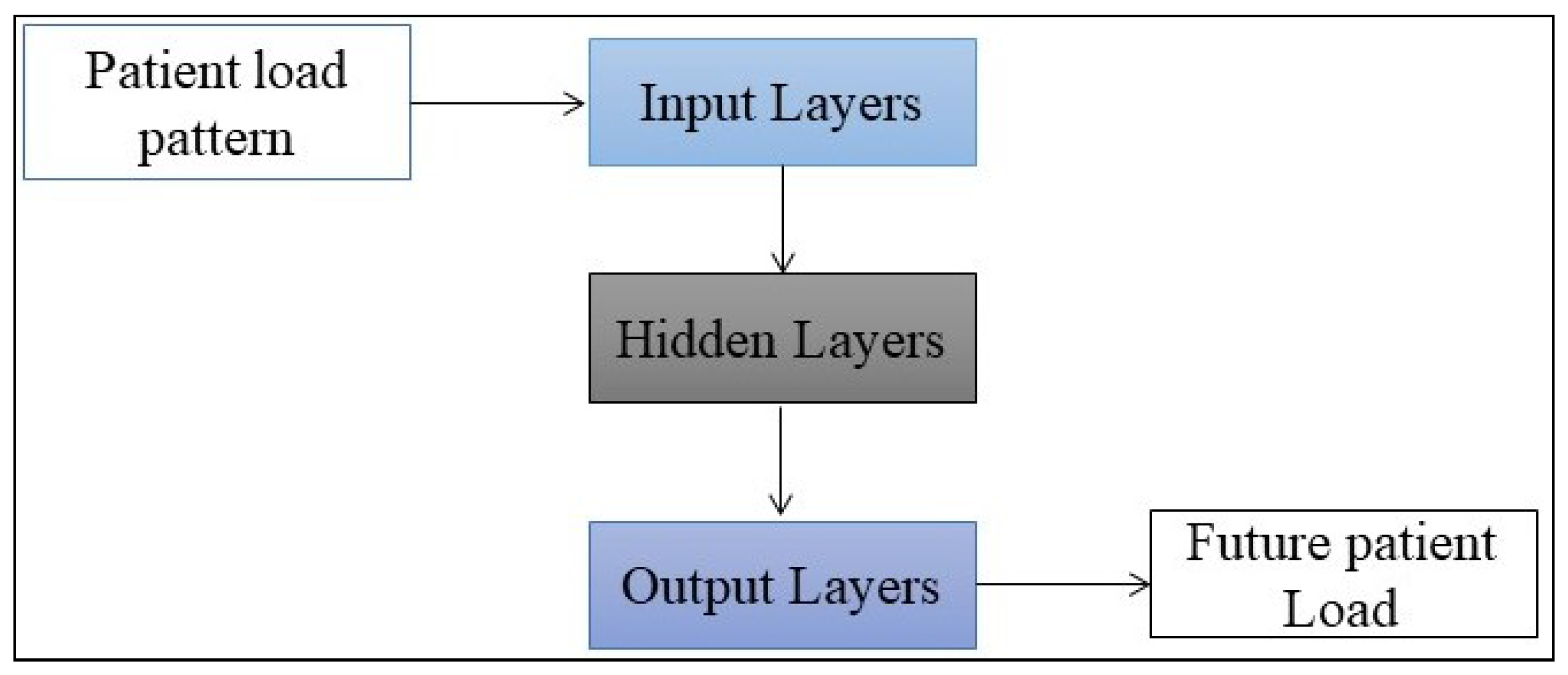
4. Proposed Deep Learning-Based Patient Load Prediction Model
The proposed deep learning-based system (
Figure 3) assumes the existence of a health information exchange (HIE) system that allows health facilities to share relevant health information. HIE systems are typically categorized by how patient health information is stored and how the participants can access patient health information [
78]. The common HIE models (from here on, we use the words model and system interchangeably) are:
Decentralized model: In this model, each participating health facility controls its data separately in special “edge servers” at a unique location. Patient-specific data is only shared with other participants upon request. In a strictly decentralized model, every request for patient data must be made to every participating data source.
Centralized model: Here participants agree to share data and the data is normalized in a common format and terminology and are housed together in a central data repository where they can be accessed and used by participants in line with agreed policies and procedures. More than one repository may exist for different kinds of data. This model may offer the best technical performance in terms of data availability and response time.
Hybrid-federated model: This model is similar to the decentralized model, but it adds a “record locator service” to track patient movement.
For our work, the required information to be shared by the health facilities is patient load information. Hence, the proposed model can suit any of the existing HIE models. However, in this work we propose two different system, a totally centralized system in which all control and computation tasks are handled by central controller and a decentralized control system.
The patient load at a health facility is influenced by the patient rate of arrival. We define the total patient load,
to be:
4.1. Centralized Patient Load Prediction System
The centralized prediction system involves four phases, namely data collection, training, prediction and online training.
4.1.1. Data Collection Phase
The Cc is responsible for collecting all information of the health facilities. Let
be the patient load sequence of every facility in the last
N time slots (or time intervals) recorded by the Cc. Let
be the collection of time intervals over which a hospital’s traffic load can be predicted. We can assume
to be hours over which the hospital is operational, say 7:00–17:00. Then let △ be the length of each time interval. Let
be the recorded patient load of a facility
i in the last time interval
k. Then the past patient load
of facility
i is given by:
which is just a length-
N vector. Where
N is the number of considered past time intervals. Note that
N depends on the complexity of the input data and is decided according to the training performance. The controller collects all patient load series of every facility and formats them as a patient load matrix:
This can also be expressed as:
Which is just a time series expression of the patient loads of all health facilities in the past N time intervals.
The patient load matrix
is the main output of the data collection phase and is taken as the input of training data. In the next time slot, the Cc records the patient load as real future patient load as:
This record is taken as the output of the training data. The process is repeated several times and the Cc gathers all such labeled data for training the deep NN in the training phase.
4.1.2. Training Phase
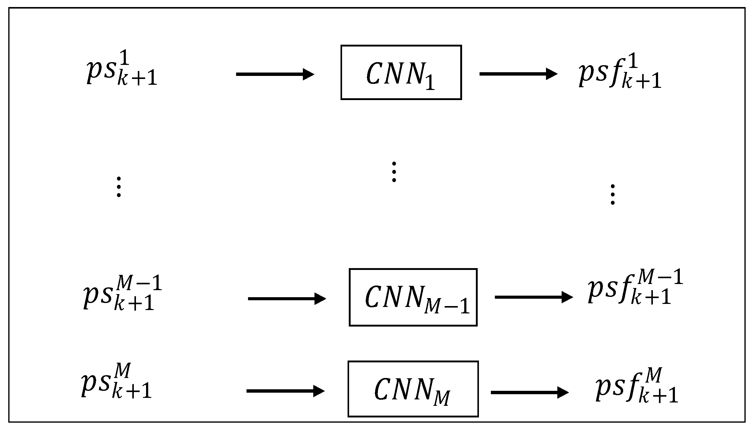
Consider M deep CNNs, with each deep CNN responsible only for training the patient load of one health facility. With this structure, the central controller takes only the future patient load of a single health facility as the output of the corresponding deep CNN. For example, take the training data of deep CNN, , . Then, the Cc trains all the deep CNNs separately so as to obtain all the stable weight matrices.
4.1.3. Prediction and Accuracy Calculation Phase
During this phase, the Cc forecasts future patient load and computes the prediction accuracy. The weight matrix of each deep CNN obtained during the the training phase is then adopted for predicting the future patient load. For all the deep CNNs, the output is recorded as:
Recall that the real future patient load of time interval
is recorded as
. Hence, the prediction accuracy can be computed according to:
where
K is the total number of time intervals considered and
is the maximum patient load of hospital
i, i.e., daily patient capacity. See
Figure 4.
4.1.4. Online Training Phase
If the arrival pattern of patient load acts in a consistent pattern/manner, then the training and prediction processes can reasonably only be based on the existing training data. It is possible, however, for the arrival pattern of patients to change because of some reasons. Under such situations, it would be important that the training process be adapted accordingly. This would necessitate the online training phase so as to allow the adjusting of the deep CNNs to adapt to the new pattern. During this phase, each health facility continuously records the patient load data and the training phase is processed periodically with the collected new training data. Hence the weight matrices are also adjusted periodically.
4.2. Decentralized Patient Load Prediction System
Unlike in the centralized system, here the Cc is granted a partial computation ability, and each health facility completes some tasks locally. Each health facility uses local information to make simple pre-forecasting. This lessens the computational burden of the Cc. The final prediction, however, is done by the Cc, but it integrates the global pre-forecasting information from all local health facilities. Below we discuss only the data collection and the training phase. The prediction phase and the online phase are the same as in the centralized control system.
4.2.1. Data Collection
In the centralized system above, the Cc predicts the patient load based on collected patient flow patterns of all health facilities. However, in the decentralized system, the Cc has limited capabilities, such that each facility does not transfer all the raw patient flow data to the Cc. Here, each facility performs some pre-processing of the raw patient flow data and sends limited/less information to the Cc, hence reducing the computational and signaling overheads of the Cc. Each facility i captures the patient load of the previous time interval and also separately captures the relayed patient load and the regular patient load from its catchment area as of the last N time slots. Using as the input, each facility i predicts the future regular patient load of the next time slot. The training and prediction process is conducted in the training phase. Thereafter, each facility forwards the obtained and the recorded patient load of the previous time slot to the Cc. The received information from all health facilities is then constructed by the Cc as the training data and .
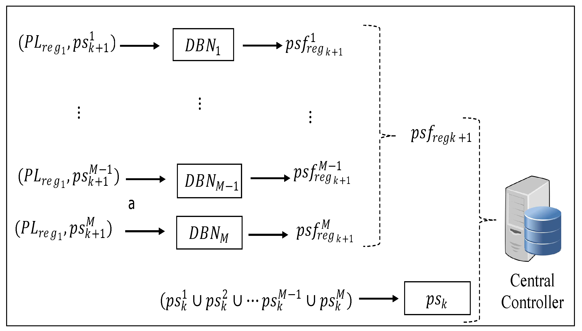
4.2.2. Training Phase
Here the training phase is split into two steps. The first step involves each health facility training a local NN to forecast its future integrated patient load with its past
N time slot regular patient loads, such that, for each facility
i, the training data of its local NN can be represented as:
Compared with the input to the deep CNN used in the Cc, here the input is simpler such that the training can be treated as a function fitting process between inputs and outputs. Hence, the DBN can be used to perform the training process. As pointed out above (i.e., in the data collection section), it is the trained DBN that will be used to forecast the future integrated patient load that is denoted as . The outcome of this process is periodically sent to the Cc.
Upon each facility completing self prediction and sending the result to the Cc, the Cc performs the final prediction with the last time interval’s patient load
and the predicted regular patient load
of all health facilities. Since the patient load and regular load are different system features, they can be considered as two separate pieces of input data. Hence, the training data input can be formed as a matrix:
As pointed out above, the deep learning structures in the Cc are used for predicting the future patient loads of all the health facilities. Just as with the central-control-based prediction, we make use of
M deep CNNs to make the prediction to reduce the computational burden and guarantee the accuracy. Hence, for
, its labeled training data is formed as (see
Figure 5):
5. Computational Considerations
A common challenge in applying machine learning techniques to problems is the exponential increase of the size of training data and the growing model complexity. It is true that the availability of large sized data requires the use of more complex machine learning models so as to discover finer structures in the data. However, more complex models are often associated with higher computational costs. Furthermore, deeper NNs also bring in more complex computational patterns [
79]. Techniques such as, shrinking the model, data parallelism and model parallelism are being explored as possible solutions to accelerate the performance of deep learning models. In [
80] it was shown that about 80% of the computational cost in NNs results from the convolution operation [
81]. Hence, recent studies on NN model designs have focused on how to configure convolutional layers [
82]. Thus to control the execution overhead of an NN model, in [
83], the authors mathematically formulate the convolutional overhead. Without such a formal overhead formulation, an NN model structure is mainly configured based on a designer’s experience with balancing the execution overhead and the model’s accuracy. The designer manually selects a configuration (based on experience or some public models) and then trains the model. In the case of low training accuracy, a different configuration will be tested. Clearly this approach lacks a systematic way to configure the model. On the contrary, with the execution overhead formulation, this configuration can be quantitative and effective. Denote
as the convolutional overhead, such that:
where
is the preferred or predefined resource budget and
is the percentage of computations due to convolution. Hence, the execution overhead of layer
k, denoted
, needs to satisfy:
where
indicates the computation percentage of each layer,
. For a detailed discussion on this method we refer the reader to [
83].
6. Patient Transfer Logistics
This section presents the development of the IoT-based smart bus system which can support the timely movement of reassigned patients from a bus stop near the source facility to the destination facility. This can help prevent putting a further strain on the already fragmented ambulatory services in many clinics. Since upon arrival patients are triaged and get treated in order of urgency, then in order of arrival, the patients that are re-assigned are the least critical, such that they can manage to carry themselves to the nearest bus station.
Hospital logistics generally differentiate between three main flows: Patient, information and material flows. The patient flows run in three directions: Towards the hospital or inbound, within the hospital or internal and away from the hospital or outbound. As pointed out above, the goals of the above proposed system are to predict future patient loads. Furthermore, in the case of excess patient loads, we propose that excess loads should be re-assigned to nearby facilities that have a minimal load as a way to control overcrowding and reduce the number of patients that leave health facilities without receiving medical care. However, the re-assigning of patients will imply a need for transportation for the patient to move from one facility to another. The two most commonly employed modes of transfer of patients are ground transport, with the inclusion of ambulances, and mobile intensive care units (MICUs) [
84]. Here we assume the existence of a scheduled bus transport system. A bus journey involves such stages as waiting, queuing and transferring from the origin point to the final destination. These stages are impacted by the services rendered and transportation network resources. Three stages exist at which transit services can affect passengers [
85]. These stages are:
Origin-point stage: At this level, passengers wait for the next bus. Passenger waiting time can be longer than expected due to irregular headway or technical issues that might affect the bus. Moreover, all passengers may not board the arriving bus due to capacity limitation. Upon being queried, the proposed smart bus system will provide passengers with information regarding the position of the bus, travel time estimate and information about the number of vacant seats in the bus. This information will help passengers to plan their waiting time accordingly.
Boarding stage: At this stage, the passenger services time (PST) is a function of passenger demand. A boarding passenger’s wait-time must allow passengers in the bus to alight. Here, we assume that near each health facility there is a boarding stage.
Arrival stage: The arrival stage is the stage where passengers reach their final destination. Their arrival can be on time, ahead or delayed based on the deviation from the timetable. For the patients, the arrival stage will be the stage near the destination facility where the patient has been referred.
Various solutions exist that are used to track data related to the departure and arrival times of buses. Radio frequency (RF) transceivers [
86] are installed on buses and bus stops to enable buses to communicate their location to bus stops. The estimated arrival time of the bus is calculated by microprocessors at the bus stops. The calculated time is displayed on screens that are installed at the stages. Some solutions employ SMS services on global system for mobile communication (GSM) modules to transmit bus positions to databases. GPS tracking devices are mounted on buses to provide location data. Sending of data to the database is via the hyper text transfer protocol [
87,
88]. Alternatively, location data can be streamed from android devices in the bus. The bus location and travel time approximation can be accessed through android devices or web portals. Unfortunately, some of these systems cannot handle an increase in requests. The bandwidth demand for sending the data from buses to servers is high. Hence, there is need to explore scalable and efficient solutions [
89].
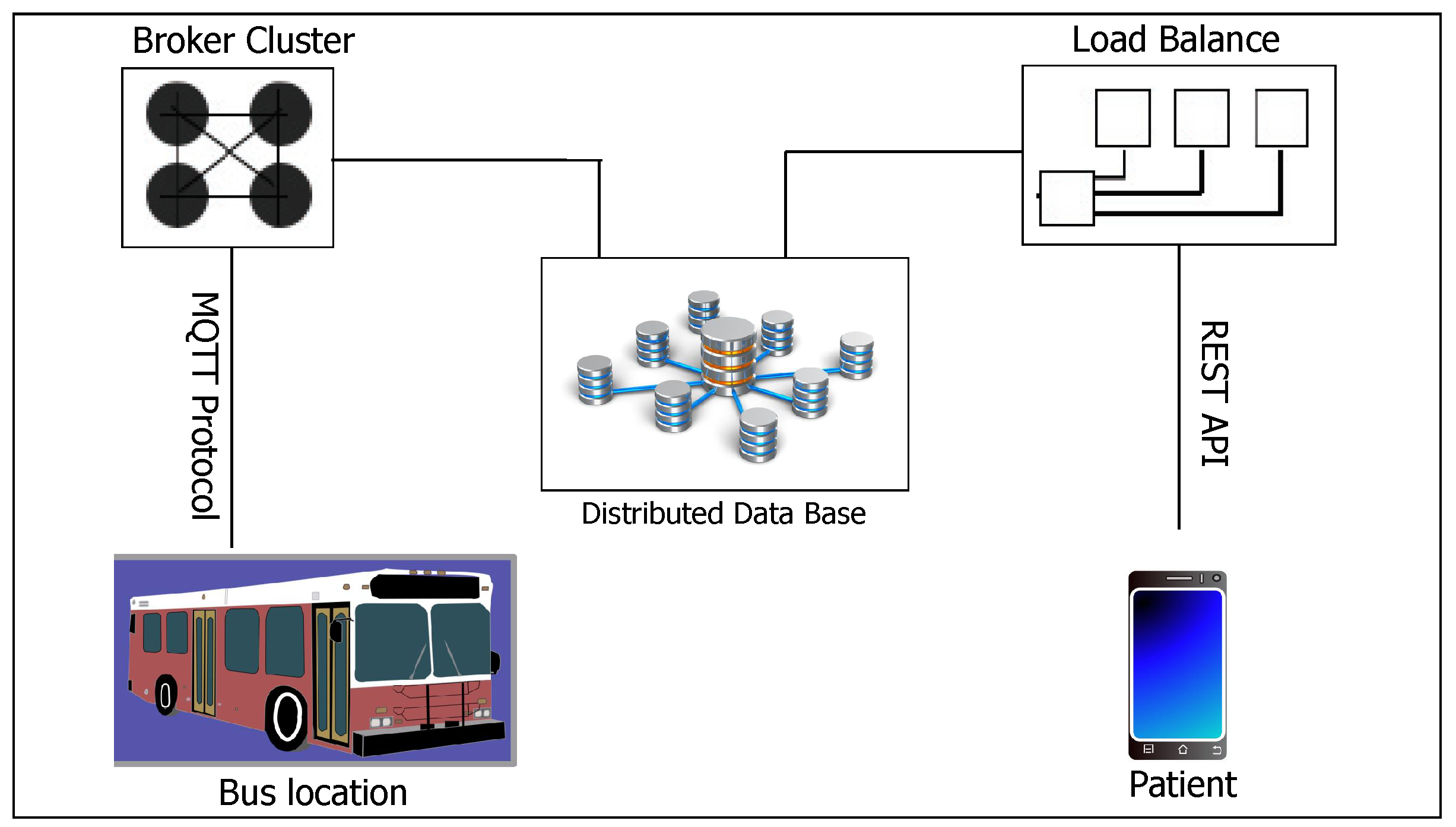
6.1. System Architecture
This section discusses the overall system architecture of our proposed smart transport system.
Figure 6 shows the proposed system architecture. Each public bus is attached with an IoT smart transport kit which comprises a variety of modules including the GPS module and two sets of laser lights with light dependent resistors (LDRs) positioned at the back and front entryway of the bus, respectively, and a smart phone that acts as a mobile hotspot. Both the GPS and the laser light with an LDR read and feed real-time data to an Arduino Uno microcontroller. The Arduino Uno connects to the Internet via NodeMCU, which sends the collected data to an MQTT broker on the cloud using the Wi-Fi provided by the mobile hotspot that provides the Internet connection. Since the smart buses will also be servicing patients, the system will need to be reliable. The patients need to accurately know the arrival time of the bus at a bus stop and the time it will reach the destination and also the status of the capacity of the bus (whether it is full or there are vacant seats in the bus). Using the real time location of buses, it is possible to calculate the approximate time for the bus to reach a particular position. This is possible since a bus’s location data can be saved on the server together with corresponding timestamps. To count the number of passengers alighting and boarding, we make use of the laser beam. The choice of the laser is motivated by the fact that it does not scatter and is invisible. Since passengers queue and enter or exit the bus one by one, with the laser, the system will not miss any passenger. Hence the counter will be reliable.
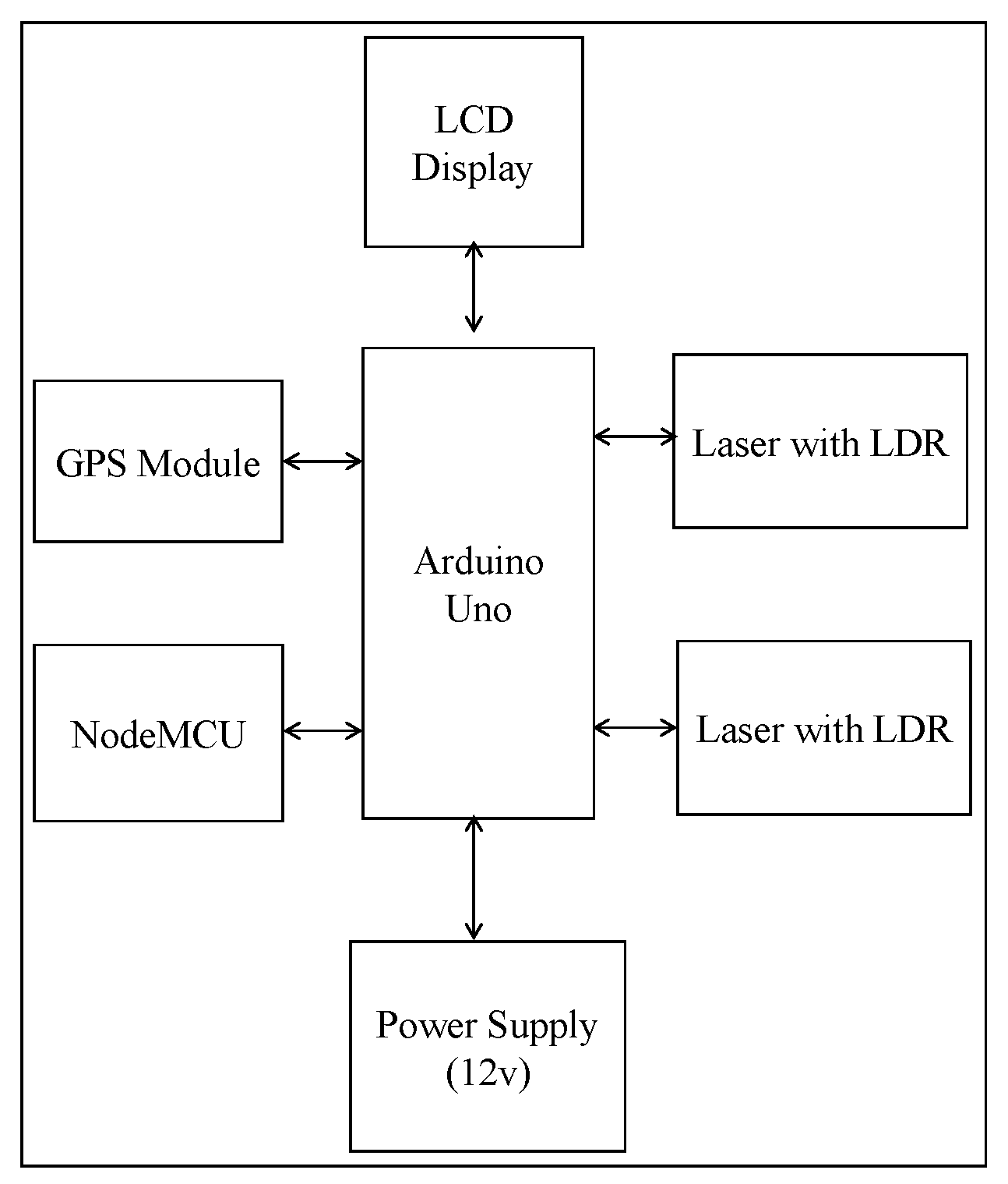
As pointed out above, each of the public buses will be tagged with an IoT-based smart bus system.
Figure 7 shows the framework of the developed IoT kit. We briefly describe the function of each of the components of the system.
Arduino Uno: This is the heart of our framework. It works as a CPU unit. Arduino Uno will generate sensor data that will have to be sent to the server. This data will include the location data of the bus, time and distance approximation of departure and arrival and also information about the capacity of the bus. Arduino will take these data and send them to NodeMCU over a serial connection.
Laser: A laser is a device emitting light through optical amplification based on the stimulated emission of electromagnetic radiation. The term “laser” originated as “light amplification by stimulated emission of radiation” [
90]. The primary wavelengths of laser radiation for most current applications include the ultraviolet, visible and infrared regions of the spectrum. Ultraviolet radiation for lasers consists of 180 and 400 nm wavelengths. The visible region lies between 400 and 700 nm wavelengths. The infrared region of the spectrum consists of radiation with 700 nm and 1 mm wavelengths. When the intensity of the radiation is sufficiently high, damage to the absorbing tissue may happen [
91]. In the proposed system, the primary functionality of the laser technology is to detect motion (i.e., entry and exist of passengers) and serve as a counter to determine the number of vacant seats in the bus. The counting starts when there is a discontinuity in the laser beam falling on the sensor. The discontinuity is detected at the entrance (or exit) of the door of the public buses at the instant of time where the laser beam is not being felt on the sensor. Here we utilize the laser technology whose path is invisible.
NodeMCU: NodeMCU is a development board that incorporates the ESP8266 Wi-Fi chip. The ESP8266 is programmable like any other microcontroller. Since Arduino Uno does not have network capabilities, the NodeMCU interfaces the Arduino Uno microcontroller, connects the system to the Internet and drives the output for the GPS and the lasers. The Wi-Fi connection is provided by the mobile hotspot that is fixed in each bus. An application server implemented using Node.js collects the data from the MQTT broker through the publish/subscribe mechanism and saves the data using the NSQL Couch DB database.
GPS receiver: GPS is a space-based radio navigation system that broadcasts highly accurate navigation pulses to users on or near the Earth. This system is used to collect the real-time co-ordinates for the system. The GPS receives the satellite signals and then the position coordinates with latitude and longitude are determined by it. The location is determined with the help of GPS and the transmission mechanism. After receiving the data, the tracking data can be transmitted using any wireless communication systems. These units are connected at the output of the system. The GPS port is serially connected with the system.
6.2. MQTT Protocol
The message queuing telemetry transport (MQTT) is a client server publish/subscribe messaging transport protocol. It is lightweight, open, simple and easily implementable. MQTT is ideal for use in IoT applications that require a small code footprint and/or network bandwidth as a premium. The protocol runs over network protocols that provide ordered, lossless, bi-directional connections, e.g., TCP/IP. In the MQTT protocol there is a broker and a receiver. The broker has `topics’ through which a recipient of data generated by a sender is determined. To receive the data, a receiver subscribes to a particular topic. A receiver receives the data published by any sender with that particular topic [
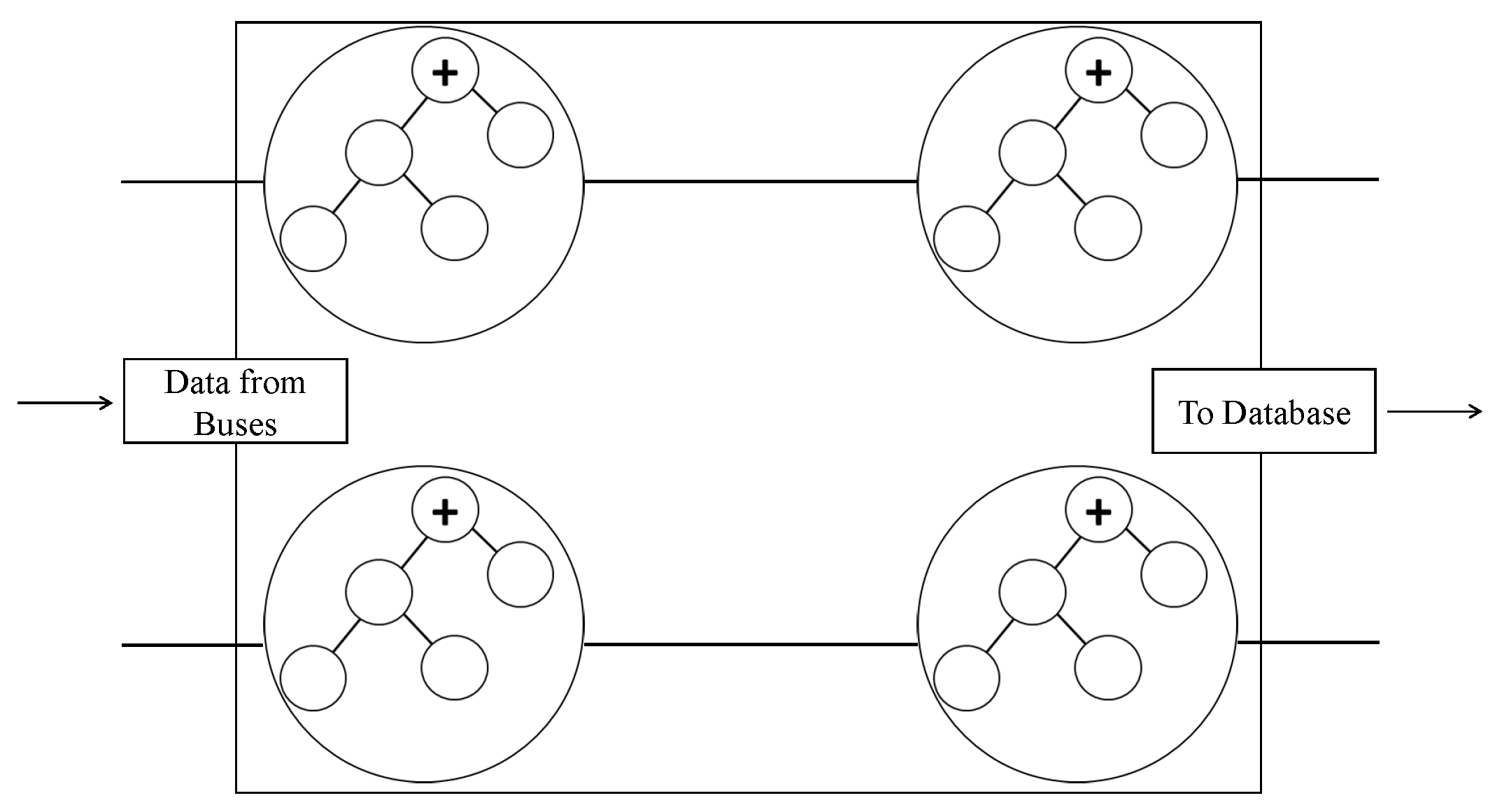
92]. In the proposed system, the topic will be the route number/name, such that the published location data from buses will contain this information. The location data will comprise the current latitude and longitude of a bus and will be published at a frequency of 5 s. To ensure the scalability of the system, the MQTT brokers can be clustered as in
Figure 8. Each of the brokers maintains the same topic list . In case of one broker crushing, another broker automatically handles the requests, balancing within themselves. The advantage of clustering is the assured system availability. For each route number, the location data is received via MQTT and stored in the database. The broker can be directly modified to write to the database upon reception of data or an MQTT client can be created to perform this function.
6.3. Data Access by Users
Various platforms can be used to enable user access to the system including web, smartphones or . The proposed system allows users to access the data via Representational state transfer (REST) APIs. HTTP requests are sent to the server and the server returns fetched data based on user context. The location information can easily be shown to users via Google maps or an equivalent map service. Through a simple application, patients and general passengers can easily search a bus by bus number directly. In case the user is not aware of the bus number, he/she will be asked to first select the nearest bus stage (i.e., the boarding point). The process can easily be automated by keeping a database of bus stops along with their corresponding location data. Distance to the the system is calculated by comparing a user’s location to that of the bus stops, applying the Haversine formula:
User latitude
User longitude
Bus stop latitude
Bus stop longitude
Earth’s Radius.
Then
From Equation (
18) above, the nearest bus stop will be the one with the shortest distance. The live location of a bus is queried based either on target destination or bus number. If the user enters a bus number, the user API returns the last known bus location from the central buses collection. To allow mapping of the boarding stop–destination point to the route number, a database of all buses on all routes can be maintained. Hence, if a user selects a boarding point and a destination point, he/she gets a live location of all buses on a route that takes him/her to the destination.
In
Table 2 above, the first row shows the route numbers, whilst the corresponding columns list bus stops on that route. For example, if a passenger queries data by boarding and destination bus stages, the query is then checked in the table. Take stops
B and
A where
B is the boarding stage and
A is the destination bus stage. The system simply checks the table to verify if bus stop
B occurs in the table and is followed by
A. However, bus stop
A need not immediately follow
B. In
Table 2, we see that routes number 101, 201 and 301 have such conditions. The query will then fetch the live locations of the buses on these three routes and return them to the user. The queries from the user module will be the same across all platforms. The output for the HTTP GET request will take the following formats.
Query by registration number: The query by registration number will return a JavaScript Object Notation (JSON) response fetching data from ‘buses’ collection with the parameters latitude, longitude, bus registration number, bus route number, direction and time stamp.
Query by route number: The query by route number will return a JSON array containing objects, with each of the objects giving details of active buses running on that route. The data will be fetched from a collection with the name ’route number’.
Query by boarding point and destination: This query will return a JSON array containing objects for active buses on every route, from the boarding point to the destination. This data will be fetched from various collections based on which routes are applicable.
6.4. Functionality Principle of the Counter
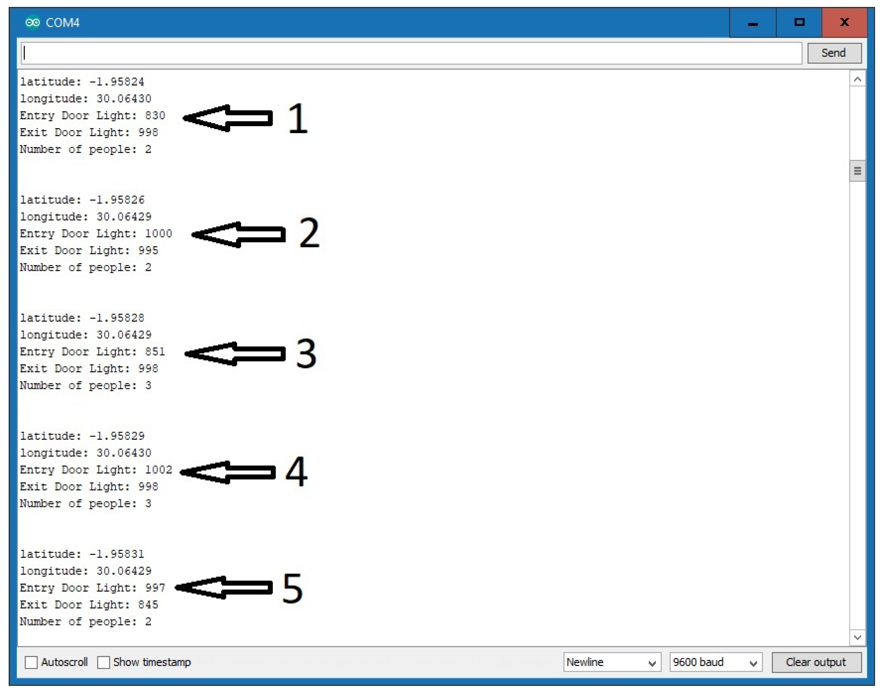
Figure 9 is the snapshot showing the system transmitting captured data. As pointed out above, the LDR (light dependent resistor) detects the increase in the intensity of the light if the laser is pointed directly at it. When there is an obstacle between the laser and the LDR, the LDR detects a decrease in the intensity of the light. Hence, by counting each decrease in the range of the optimum level, the system is able to count passengers entering and exiting the smart bus. From
Figure 9, as per our simulations, the maximum light intensity of both the entry and exit doors’ LDR is set at ≥900 such that any value of <900 signifies an obstacle and in our case this will signify a passenger leaving or entering the smart bus. From part 2 in
Figure 9, we see that the number of passengers in the bus is 2 and the light intensities on the LDR for the entry and exit doors are 1000 and 995, respectively. Since both are above 900, this means there is no entry or exit of passengers from the smart bus. In part 3 of
Figure 9, we observe that the light intensity for the entry door is <900 and this decrease corresponds to the increase in the number of passengers, which has increased from 2 to 3. For this simulation, the smart kit was stationary; hence, the fixed latitude and longitude values are
and
, respectively.

 ,
, 


