1. Introduction
In the field of computer vision, human action recognition in videos has become one of the most researched areas because it has a wide variety of applications such as surveillance, robotics, healthcare, video searching, virtual reality, and human–computer interaction [
1]. However, recognizing human actions from a video stream is a challenging task. First of all, video-based human behavior recognition has a somewhat complicated motion background. The high complexity and variability of human motion make it difficult to recognize movement correctly. Second, unlike image data, video data also contains temporal information, which is very important in video classification.
Nevertheless, the field has achieved significant success in recent years. Motivated by the success that has been achieved with deep learning methods such as convolutional neural networks (CNNs) [
2], used in image and video classification [
3], there is an increasing interest to apply that approach in the action recognition field as well. Simonyan et al., [
4] first applied the proposed two-stream network to the field of video behavior recognition; separately acquired the video image information and optical flow information of the video and trained the CNN model; and finally merged the two branches. Feichtenhofer et al., [
5] replaced the basic spatial and temporal networks with a VGG-16 network on the basis of two streams, which further improved the effect. The TSN network proposed by Wang [
6] further improved the two-stream network by using the input combination of RGB, optical flow, and warped optical flow in addition to the the network structure using BN-inception. To improve network accuracy by deepening the network layers, ResNets [
7] and Highway Networks [
8] bypass signals from one layer to the next via identity connections. Stochastic depth [
9] shortens ResNets by randomly dropping layers during training to allow for better information and gradient flow. FractalNets [
10] repeatedly combine several parallel layer sequences with different numbers of convolutional blocks to obtain a large nominal depth while maintaining many short paths in the network.
In fact, a direct method of action recognition using deep networks is to use temporal information to arm the convolutional operation. To achieve this, Huang et al., [
11] presented a three-dimensional (3D) convolutional network using 3D convolution operations to extract features from spatial and temporal dimensions to capture spatiotemporal information between adjacent frames. Although the 3D convolutional network has a simpler design idea, it generates a large number of intermediate parameters, which increases the complexity of the network.
Recently, DenseNets [
12] have attracted significant attention from computer vision researchers due to their dense connections. This network has shown impressive performances in natural image classification tasks. The network connects each layer to any other layer in a feed-forward manner. This dense connection structure can facilitate gradient flow during training. Compared with the 3D convolutional neural network, the dense connection of DenseNets reduces the repeated calls of intermediate parameters, which can reduce a large number of network parameters, thus reducing the complexity of the network. However, DenseNets have only been applied in terms of images; they have not performed well in the video field.
It is well known that deep convolutional neural networks (DCNN) [
13] require a fixed-size image input. This requirement may affect the recognition accuracy for the images or sub-images of an arbitrary size/scale. However, in reference [
14], the authors present a spatial pyramid representation method. In this method, the fixed-size constraint can be removed by using the spatial pyramid pooling (SPP) model.
Inspired by the application of SPP in the image field, the image cropping is reduced, thereby reducing the loss of image information. Can the video field also reduce such information loss? What would be the effect of applying SPP to the video world? Considering the advantages and disadvantages of both 3D convolutional neural networks and DenseNet networks, combined with the SPP network model, we propose a new network model and employ it in experiments based on video information behavior recognition.
In this paper, a novel network architecture based on 3D convolution network, densely connected convolutional networks, and the Spatial Pyramid Pooling network is proposed. We call it “3D-DenseNet-SPP”. In this architecture, we take DenseNet as the primary network structure. By adding time module information to the DenseNet, we can achieve the purpose of integrating DenseNet with a 3D convolution network, so that it not only makes full use of temporal and spatial features but also reduces the gradient vanishing and reduces the training parameters of the network to a certain extent, as compared with the 3D convolution network alone. Then, by the network structure, we add the spatial pyramid pooling model to satisfy the input of any scale/size.
2. Related Works
2.1. D Convolutional Neural Networks
3D convolution neural network can not only extract the spatial features from the local neighborhood on feature maps in the previous layer, but also obtain the temporal features between adjacent frames. Overall, the 3D convolution neural network is performed to extract spatial and temporal features from video data for action recognition. Its excellent performance benefits from 3D convolution operation and 3D pooling operation.
3D convolution. 3D convolution is achieved by convolving a 3D kernel to the cube formed by stacking multiple contiguous frames together. By this construction, the feature maps in the convolution layer are connected to multiple adjacent frames in the previous layer, thereby capturing motion information.
3D pooling. Usually, to reduce the network parameters and the spatiotemporal size of the video representations, we need to add a 3D pooling layer between 3D convolution layers. The 3D pooling operation simply involves adding the temporal dimension to 2D pooling. Pooling operations have many types, such as maximum pooling, average pooling, and L2-norm pooling. In a 3D convolution neural network, 3D pooling operation can not only reduce computation but also control overfitting.
2.2. Spatial Pyramid Pooling
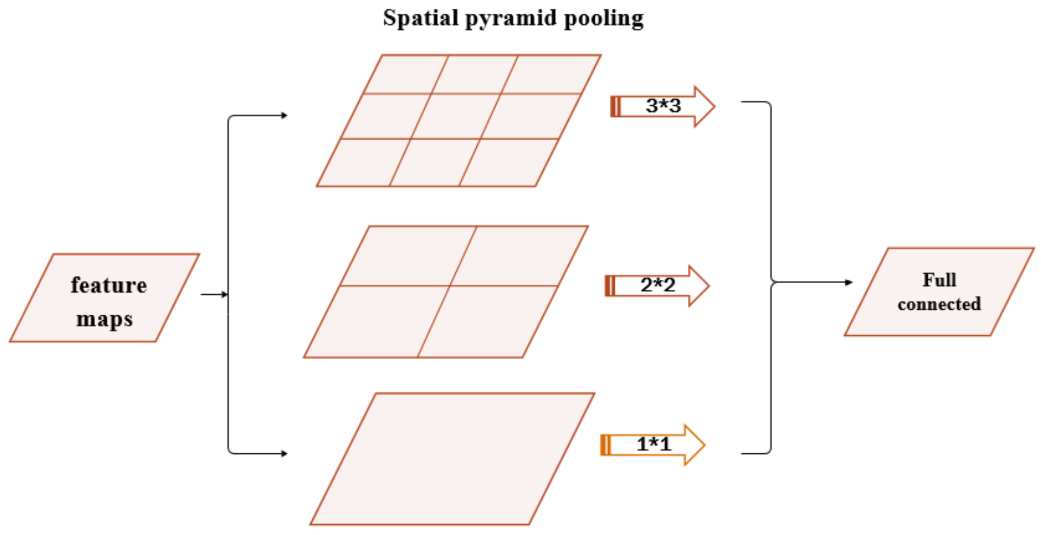
The spatial pyramid pooling model (SPP) can maintain spatial information by pooling in local spatial bins. The size of these spatial bins is proportional to the image size, so the number of bins is fixed regardless of the image size. This is in contrast to the sliding window pooling of the previous deep networks, where the number of sliding windows depends on the input size.
Generally, to make deep networks adapt to input images of any sizes, the spatial pyramid pooling uses multi-level spatial bins to substitute max-pooling layers or average-pooling layers, which has been shown to be robust. The structure of SPP is shown in
Figure 1. In each spatial bin, the response of filters is randomly pooled. In SPP, the output of each pooling level will eventually be exported to the full connected layer in parallel. For example, if there are
N bins, the outputs of SPP are the
kN-dimensional vectors with a fixed length, where
k denotes the number of filters used in the last convolution layer. The vectors in fixed dimensions are the inputs of fully connected layers.
Besides, if the size of the feature maps from the previous layer is
a a, at the pyramid level of the size of
n n bins, the size and stride of the filters are respectively calculated by:
where
and
are defined as the ceiling operation and floor operation, respectively.
2.3. Densely Connected Convolutional Network
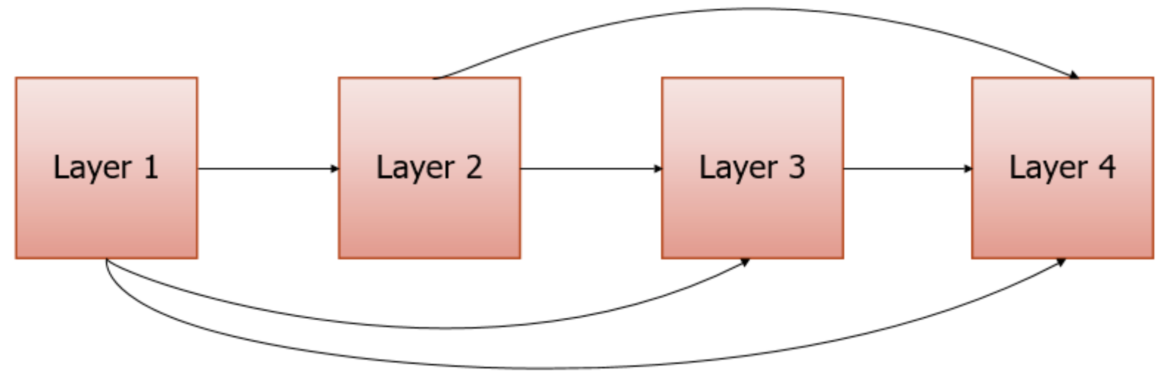
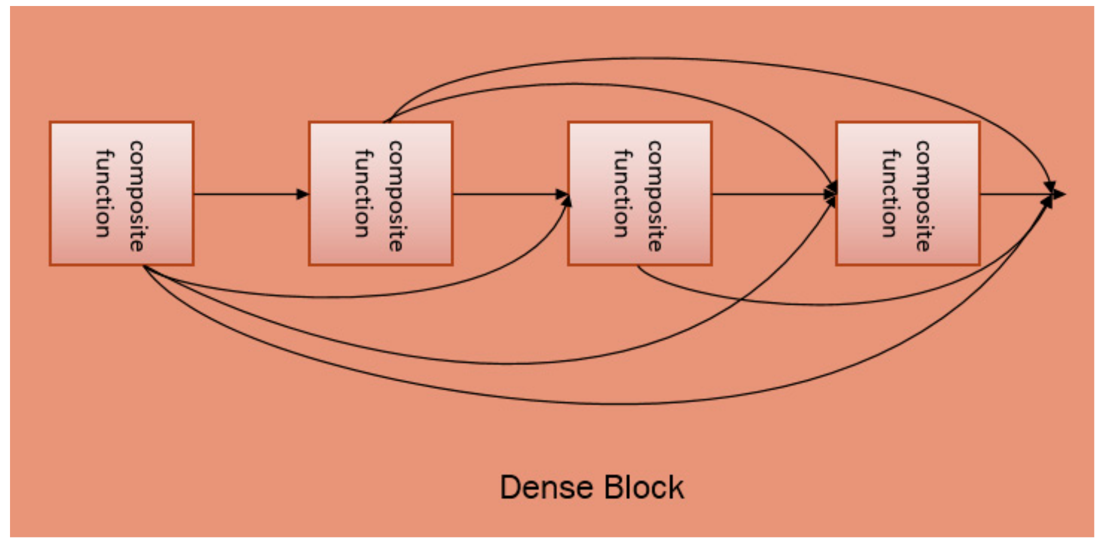
A densely connected convolutional network (DenseNet) is a convolution network for image classification. Usually, when a convolution network is deeper and deeper, the information of input and gradient will gradually disappear after passing through several layers. However, this problem can be solved by DenseNet with dense connections. It directly connects all the layers in the network using the same size feature maps to ensure the maximum information flow between the layers. Each layer requires information from all previous layers as input, and then it passes its feature maps to all subsequent layers. By using dense connections, the DenseNet architecture allows for better information and gradient flow during training. The dense connections structure is shown in
Figure 2.
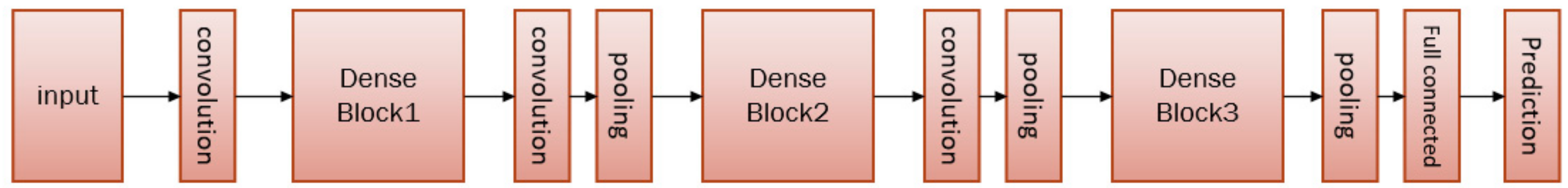
The DenseNet is mainly composed of several dense blocks and transition layers as a whole. Each dense block contains several composite functions. These composite functions are connected to each other through dense connections. The composite function consists of three consecutive operations: BN [
15], followed by ReLU [
16], and finally a convolution layer. ReLU is an activation function of the CNN, which is defined as:
where
x is the output of the BN. ReLU has the advantage of reducing the likelihood of a vanishing gradient without affecting the receptive fields of the convolution layer. Compared with other activation functions, ReLU has faster speed and better accuracy.
Layers between each dense block are transition layers, which perform the convolution and pooling operations. The overall architecture of DenseNet can be found in
Figure 3.
3. Methods
3.1. Model Structure
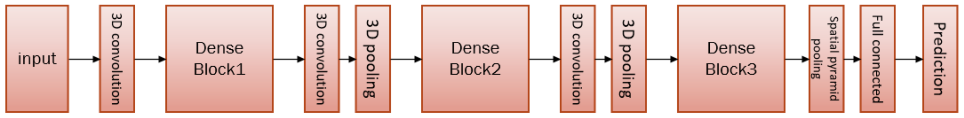
Inspired by the spatial pyramid pooling model applicable to images of any size, as well as the recent success of densely connected networks in image classification tasks, we propose a new neural network structure, that is, a 3D DenseNet based on spatial pyramid pooling (3D-DenseNet-SPP) that is able to work on an action recognition task. In our model, we use the DenseNet as a major network branch and add the corresponding 3D module to it in order to form the 3D DenseNet. In the 3D DenseNet, the last pooling layer (the former pooling layer of the full connection layer) is replaced by the spatial pyramid pooling layer. In addition, each layer of the SPP represents average pooling. The structure of our model is shown in
Figure 4.
Before introducing our model, we introduce some related concepts: dense connectivity, composite function, and growth rate.
Dense connectivity. Dense connectivity is the direct connection from any layer to all subsequent layers. The purpose of dense connection is to improve the information flow between layers so that it has fewer network parameters and a faster running speed. (The layers are interconnected and can be reached directly through each other. There is no need to transition through the middle layer, so the speed will be faster). This structure can be found in
Figure 2.
Normally, suppose
is the output of the
th layer. In the traditional feed-forward networks, the output
is computed by:
where
is a non-linear transformation of the
th layer. Usually, this way cannot avoid gradient disappearance or explosion, especially in deep neural networks. However, in the structure of dense connections, the
th layer needs to send the feature maps
to all subsequent layers. In turn, layer
l will receive feature maps from all preceding layers as input:
where
is the concatenation of the feature maps produced in layers 0, 1,
,
l − 1.
refers to the composite function. By using dense connections, the DenseNet architecture allows better information and gradient flow during training. In this paper,
contains not only spatial information but also time information.
Composite function. The composite function consists of three consecutive operations; namely, BN, ReLU, and 3D convolution. To reduce the transfer of internal covariates, the BN layer is added before the ReLU layer of each composite function. The input of the ReLU layer is the output from the BN layer, while the output of the ReLU layer is used as the input of the 3D convolution layer.
Growth rate. An important difference between DenseNet and existing network architectures is that DenseNet can have very narrow layers. If each composite function of layer l in Equation (4) produces k feature maps, then the lth layer has input feature maps, where is the number of channels in the input image of the video clip. To prevent the network from developing too fast, k usually takes a smaller value, e.g., k = 12, and the hyper-parameter k is the growth rate.
In this model, we can perform a local perception of spatial information and time information through 3D convolution, and quickly acquire spatiotemporal features through a parameter sharing mechanism. Through the feature integration of the pooling layer, we can prevent overfitting and improve the generalization ability of the model while also reducing parameters and unnecessary calculations. By using spatial pyramid pooling, we can avoid image clipping and unnecessary information loss. Finally, at the fully connected layer, the extracted features are used for classification.
3.2. Model Details
In our model, to make better use of 3D convolution and 3D pooling, we take the multiple densely connected dense blocks. More dense blocks will cause the network to become deeper, which will increase the parameters and complexity of the network. On the contrary, if the selected dense block is too small, the number of layers of the network will be reduced, which will affect the accuracy of the model.
In our experiment, Due to GPU memory constraints, we use three dense blocks. Each dense block contains several composite functions that are connected in a feed-forward manner. The structure can be found in
Figure 5. The feature maps of all the preceding composite layers are concatenated in series along the last dimension and are used as the inputs for current composite function. The output feature maps are also used as inputs for all subsequent layers. Between the two adjacent dense blocks is the 3D convolution layer and the 3D pooling layer. As transition layers, they are mainly used to resize the feature maps to realize the down-sampling. The last layer is a fully connected layer that creates a connection between the feature maps and the different type of actions. Before the fully connected layer is a spatial pyramid pooling layer, which is used to meet the needs of images of any size.
It is well known that traditional SPP networks are used in two-dimensional network architectures. The two-dimensional feature map from the upper layer is output in parallel to the fully connected layer through the SPP structure. In our model, the three-dimensional feature map is passed into the SPP structure. In order to be able to connect properly, we add a time dimension to the traditional SPP network structure to expand it. At the same time, in order to ensure that the SPP layer is not affected by interference from the time information, spatial pyramid pooling is performed only in the spatial dimension. The time information is guaranteed to be the same at each layer of the SPP, and the spatial information is normally calculated according to the traditional SPP network.
To a certain extent, our model can be regarded as an improvement to the densely connected network model. Compared with DenseNet, our model can be used not only for the processing of 3D video data, but also for inputting video frames of any size. On the other hand, our model has fewer model parameters than the 3D convolutional neural network.
In our experiments, we used a 3D convolution layer with a kernel size of 333 on the input images before we entered Dense Block1. The output channel for this convolution layer is twice the growth rate. For each convolution layer inside Dense Block1, each side of the input is zero-padded by one pixel to maintain a fixed-size feature-map. The 3D convolution layer of the transition layer between each dense block has a size of 111. The size of the 3D average pooling layer between Dense Block1 and Dense Block2 is 1 22, and the size of the 3D average pooling layer between Dense Block2 and Dense Block3 is 222. The 3D pooling layer after Dense Block3 has a size of 22, where N is the number of images in the video clip.
4. Experiments
We used the KTH [
17] dataset and the UCF101 [
18] dataset to evaluate the proposed method. All experiments are conducted on a ThinkStation P510 PC with Intel(R) Xeon(R) E5-2623 2.6 GHZ CPU and Quadro M5000 GPU with 8 GB memory. For the KTH dataset, the average training time for each setting was 10 h. For the UCF101 dataset, the average training time for each setting was two days. Our experiments were implemented in Python2.7 with TensorFlow.
4.1. Dataset and Training
KTH. The KTH dataset contains six types of human actions with 2391 video sequences. All sequences were taken over homogeneous backgrounds with a static camera with a 25-fps frame rate. These sequences were down-sampled to a spatial resolution of 160 × 120 pixels and have a length of 4 s on average.
UCF101. The UCF101 dataset includes a total number of 101 action categories with 13,320 videos, which have divided into five types. The clips of one action class are divided into 25 groups which contain four to seven clips each. All clips have a fixed frame rate and resolution of 25 fps and 320 × 240, respectively.
In our experiments, all the dataset subjects were divided into a training set, a validation set, and a test set. The classifiers were trained on a training set while the validation set was used to optimize the parameters of each method. The presented recognition results were obtained on the test set. In the KTH dataset, all sequences were divided with respect to the subjects into a training set (eight persons), a validation set (eight persons), and a test set (nine persons). In the UCF101 dataset, we used the three splits into training and test data, and the performance was measured by the mean classification accuracy across the splits.
All the networks were trained using stochastic gradient descent (SGD) [
19]. The network initial learning rate was set to 0.1, which decreased to 0.01 at 1/2 epochs and 0.001 at 3/4 epochs. In our model, we used a weight decay of
and a Nesterov momentum [
20] of 0.9 without dampening for all the weights. The network growth rate was set to 12 or 24. The batch size was set to 4, 8, or 10 according to the growth rate and the depth of the network; the higher the growth rate and depth, the lower the batch size. In the KTH dataset, the batch size was set to 4 or 8. We trained this model for 60 epochs; we divided the learning rate by 10 at epoch 30 and divided it by 100 at epoch 45. In the UCF101 dataset, the batch size was set to 8 or 10. We trained this model for 100 epochs; we divided the learning rate by 10 at epoch 50 and divided it by 100 at epoch 75. Due to GPU memory constraints, the maximum crop size of the video (which is the height and width of the image) was set to 256
256. In the spatial pyramid pooling layer, we used a three-layer pyramid to pool the features on the feature maps. The pyramid was {3
3, 2
2, 1
1}. When the pyramid pooling layer received the feature maps from Dense Block3, the size and stride of the filters were calculated through Equation (1).
Video data includes three-dimensional information, including depth, height, and width. Therefore, when using spatial pyramid pooling, we need to consider ignoring depth information and make sure that the depth information is the same at each level of the SPP. We only need to pool on the two dimensions of height and width. Of course, we can also consider pooling directly in three dimensions. However, if this is undertaken, we need to perform spatial pyramid pooling on the spatial dimension and temporal pyramid pooling on the time dimension. This will be studied in our further research work.
4.2. Performance
In our experiments, we trained our model with different depths and growth rates. To compare with our model, we carried out a number of experiments separately through the use of spatial pyramid pooling layer and without spatial pyramid pooling (3D-DenseNet-SPP and 3D-DenseNet). The configuration of our model parameters and main results achieved with the KTH and UCF101 datasets are shown in
Table 1. The pyramid is {3 × 3, 2 × 2, 1 × 1} in the 3D-DenseNet-SPP structure described in
Table 1.
From
Table 1, we can see that 3D-DenseNet-SPP was generally more accurate than 3D-DenseNet. The maximum accuracy of 3D-DenseNet-SPP was 0.9197, and the maximum accuracy of 3D-DenseNet was 0.9110 in our experiments. As a result, the accuracy was improved by 0.87% in the KTH dataset. The recognition performance averaged across five random trials is reported in
Table 2, along with published results in the literature. We used the same training and test splits of the KTH dataset, except 3DCNN, in
Table 2. In the UCF101 dataset, we also compared two sets of experimental data. The maximum accuracy of 3D-DenseNet was 0.8738, while the maximum accuracy of 3D-DenseNet-SPP was 0.8894. The results showed that our accuracy increased by 1.56%. Therefore, the experiments showed that our model improved on KTH dataset and UCF101 dataset compared to the general 3D densely connected network. This shows that our improvement is effective.
Our model not only has considerable experimental accuracy, but also has better parameter efficiency. With the same configuration of 3D-DenseNet-SPP and 3D-DenseNet, it is clear that the parameters of 3D-DenseNet-SPP have much lower values than those of 3D-DenseNet. For example, when the depth, growth rate, and batch size are 20, 24, and 8, respectively, 3D-DenseNet-SPP has a parameter of 0.4 M and 3D-DenseNe has a parameter of 0.6 M. All of these are shown in
Table 1. This observation shows that our model can increase parameter efficiency and reach a higher accuracy with the same level of parameters.
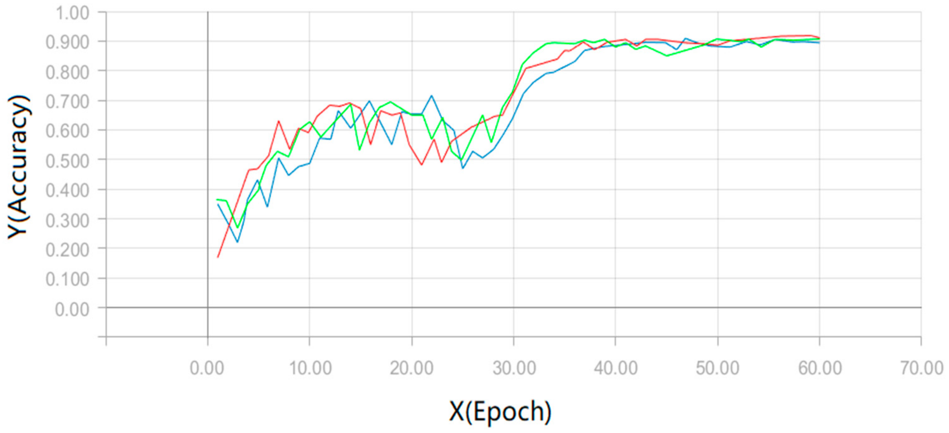
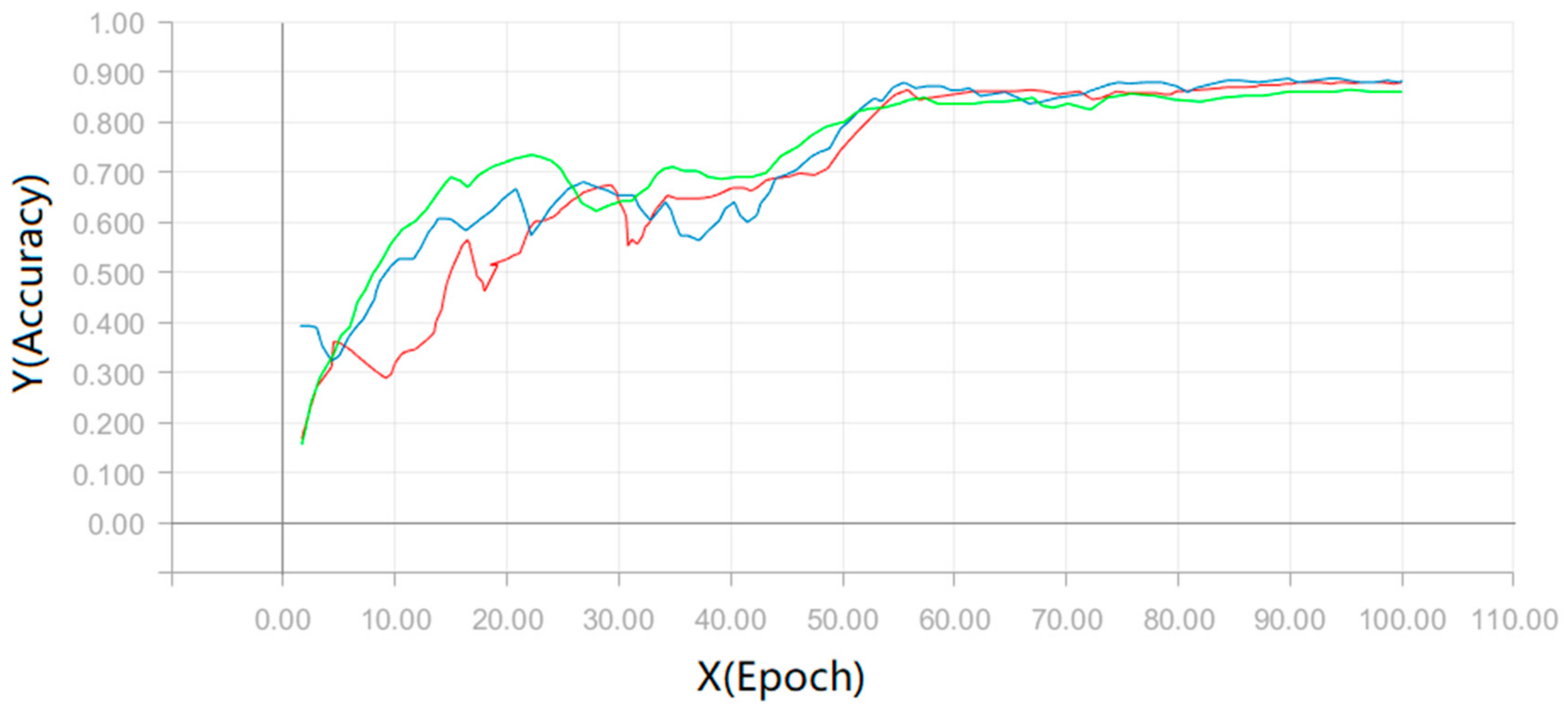
In the test, we experimented on each configuration 10 times, and then took their average as the mean accuracy of our experiment. The test mean accuracy of our model can be found in
Figure 6 and
Figure 7. In
Figure 6, we export the test results of the three sets of configurations in the KTH dataset. The three sets of configurations come from
Table 1. The red line represents the output of a network depth of 20 and a growth rate of 24. The blue line represents the output of a network depth of 20 and a growth rate of 12. The green line represents the output of a network depth of 30 and a growth rate of 12. In
Figure 7, we output the test results of the three sets of configurations on the UCF101 dataset. Similarly, these configurations come from
Table 1, where the red line represents the output of the configuration with a network depth of 20 and a growth rate of 12. The blue line represents the output of the configuration with a network depth of 20 and a growth rate of 24. Finally, the green line represents the output of the configuration with a network depth of 30 and a growth rate of 12.
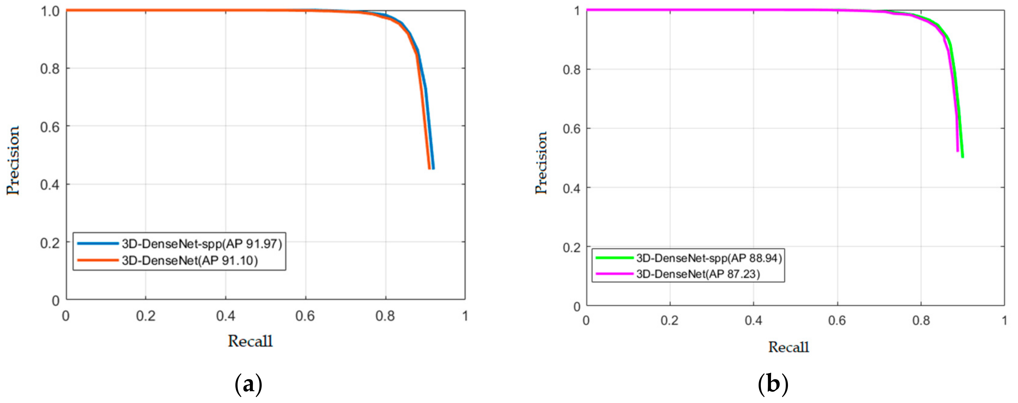
In order to evaluate our model better, we also draw the precision-recall (PR) curves. The PR curves of our approach on the KTH dataset and the UCF101 dataset are shown in
Figure 8a,b, respectively. Obviously, our model can already achieve a better performance.
Furthermore, we made some comparisons with existing models concerning accuracy. The results can be found in
Table 3 and
Table 4. The results from
Table 3 and
Table 4 show that our model has a fairly good performance. In fact, our experiments only use RGB images as input, without any data enhancement or optimization. Thus, our method has the potential to reach a higher accuracy via data enhancement measures and testing different configurations of the network.
5. Discussion and Conclusions
In this paper, the problem of video-based human behavior recognition is discussed. To better improve the recognition effect and realize video input of any size, we proposed a 3D densely connected convolutional network model based on spatial pyramid pooling (3D-DenseNet-SPP). The model is an extension of the densely connected network (DenseNet), achieved by adding time information to all convolution layers and pooling layers and adding the spatial pyramid structure. Our model was tested on the KTH dataset and UCF101 dataset separately. The experimental results showed that our model not only allows video frames with an arbitrary size to be trained, but also exhibits a better performance as compared with existing models.
In this paper, we considered the combination of the 3DCNN model, SPP, and DenseNet for action recognition. In fact, there are many other deep architectures, such as two-stream and ResNet models. These models are often used in the field of images and have better performance. It would be interesting if these models could be further extended to the video area. This potential will be explored in our future work.


