Modelling Hydrocortisone Pharmacokinetics on a Subcutaneous Pulsatile Infusion Replacement Strategy in Patients with Adrenocortical Insufficiency

Abstract

In the context of glucocorticoid (GC) therapeutics, recent studies have utilised a subcutaneous hydrocortisone (HC) infusion pump programmed to deliver multiple HC pulses throughout the day, with the purpose of restoring normal circadian and ultradian GC rhythmicity. A key challenge for the advancement of novel HC replacement therapies is the calibration of infusion pumps against cortisol levels measured in blood. However, repeated blood sampling sessions are enormously labour-intensive for both examiners and examinees. These sessions also have a cost, are time consuming and are occasionally unfeasible. To address this, we developed a pharmacokinetic model approximating the values of plasma cortisol levels at any point of the day from a limited number of plasma cortisol measurements. The model was validated using the plasma cortisol profiles of 9 subjects with disrupted endogenous GC synthetic capacity. The model accurately predicted plasma cortisol levels (mean absolute percentage error of 14%) when only four plasma cortisol measurements were provided. Although our model did not predict GC dynamics when HC was administered in a way other than subcutaneously or in individuals whose endogenous capacity to produce GCs is intact, it was found to successfully be used to support clinical trials (or practice) involving subcutaneous HC delivery in patients with reduced endogenous capacity to synthesize GCs.

1. Introduction

Glucocorticoids (GCs) are a class of steroid hormones naturally secreted by the adrenal glands of mammals. They rapidly diffuse via the bloodstream across the body, modulating multiple physiological systems, e.g., metabolism, the immune system, the nervous system, as well as under baseline and stressful conditions [1]. Due to their lipophilic nature, GCs move freely across extracellular and intracellular membranes and bind to two classes of GC-sensitive receptors: glucocorticoid receptors (GRs) and mineralocorticoid receptors (MRs) [2]. Binding events between the hormone and its receptors induce rapid, non-genomic activity of molecular signalling cascades (involving activation and inhibition of second messenger molecules such as the cyclic adenosine monophosphate) [3] as well as delayed, genomic phenomena (activation and inhibition of gene expression after interacting with GC-responsive elements) [4]. The plethora of different cellular responses to GC stimulation is particularly evident in the brain, where both major receptor types (GRs and MRs) are exposed to GCs. In other tissues, such as the kidneys, the presence of 11β-hydroxysteroid dehydrogenase 2 in the proximity of MR- and GR-expressing cells deactivates GCs, which prevents binding to GC-sensitive receptors [5].

For any brain region containing different numbers of neurons and glial cells and expressing different distributions of GRs and MRs, the type of cellular responses to GCs can be understood as a complex interplay between: (i) the concentration of the hormone in the microenvironment of that brain region and (ii) the duration of the hormonal presence in that region. For instance, when GCs are in abundance, GRs can rapidly (i.e., within seconds) be activated by GCs and subsequently bind to chromatin. However, at each of these exchange events, when GC levels fall, there is an increased probability that the hormone ligand will be lost from the GR; unbound GR will then either be metabolized by nuclear or cytoplasmic proteosome or enter the chaperone cycle, with the association of the molecular chaperones HSP90 and p23. In this state, the GR (and other transcriptional cofactors) are not associated with chromatin, and the histone acetylation state returns rapidly to basal levels [6,7]. Moreover, the binding affinities of GCs for MRs are much higher compared to GRs—i.e., lower levels of GCs are required to induce MR-dependent effects, whereas GR-dependent effects require higher GC levels [8]. Finally, prolonged exposure to high GC levels leads to downregulation of GR expression in the brain [9]. These examples indicate how important the dynamic regulation of GC levels in the microenvironment of brain cells is for determining the type of cellular responses to GC stimulation.

The delayed negative feedback loop between the control centre of GC biosynthesis (anterior pituitary) and the GC-producing tissue (adrenal gland cortex) creates a natural, ultradian rhythm of GC secretion [10]. This ultradian rhythm consists of periodic bursts of GC biosynthesis and then releases into the systemic circulation, which rapidly travels across the body (95% of which is bound to carrier proteins of the blood stream). Thus, under baseline conditions, GC-sensitive tissues (such as the brain) are exposed to short-lasting GC pulses, wherein periods of high GC levels (potentially inducing genomic and non-genomic GR-dependent and non-genomic MR-dependent effects) alternate with periods of low GC levels (crucial for resetting the afore-mentioned molecular mechanisms, i.e., sustain their sensitivity to a forthcoming GC pulse) [11]. The ultradian GC rhythm is not only significant from a physiological point of view but also from a pharmacological perspective: current GC replacement therapy does not reproduce the characteristics of complex physiological GC rhythms, leading to suboptimal treatment of patients with adrenocortical insufficiency [12].

In recent years, we conducted two clinical trials to investigate the neurobiological significance of the ultradian GC rhythm in humans, either healthy volunteers [13,14] or patients with adrenocortical insufficiency. The trial in the latter case [15] aimed at altering the HC dosing regimen to restore physiological ultradian hormonal rhythmicity. These studies were the first to show that something closer to physiological HC delivery might improve brain function in patients and offer a better self-perceived sense of well-being and quality of life. In both studies, we used a novel pump of sub-cutaneous HC delivery (Crono P^®, CANE Applied Medical Technology Ltd., Cambridge, UK), programmed to deliver 8 HC pulses every three hours at a rate of 10 μL/s [14], and in particular 400 μL solution (containing 4 mg of hydrocortisone) at 03:00 a.m., 06:00 a.m. and 09:00 a.m., 230 μL solution (containing 2.3 mg of hydrocortisone) at 12:00 p.m., 15:00 p.m., and 18:00 p.m., and 50 μL solution (containing 0.5 mg of hydrocortisone) at 21:00 p.m. and midnight. A preliminary validation study preceded these trials to verify that pharmacological interventions involving the Crono P^®-mediated HC delivery could achieve the desired GC dynamics in the blood stream [16].

The dynamics of GCs in the systemic circulation created by the Crono P^® under different settings has been previously monitored through daily blood sampling sessions with a 10 min sampling rate, as well as a subsequent determination of plasma cortisol levels. However, this process is enormously labour-intensive for both examiners and examinees and its feasibility is questionable under certain experimental settings (e.g., multimodal neuroimaging studies that can take up to two hours, including preparation of the participants, potential cognitive training, scanning and/or neurofeedback session). Thus, the aim of this work is to provide a mathematical model that describes the pharmacokinetics of the subcutaneous delivery of HC doses through the Crono P^®. We show how this model can be used to approximate the values of plasma cortisol levels at any time point of the day using only a limited number of plasma cortisol measurements as model inputs.

2. Results

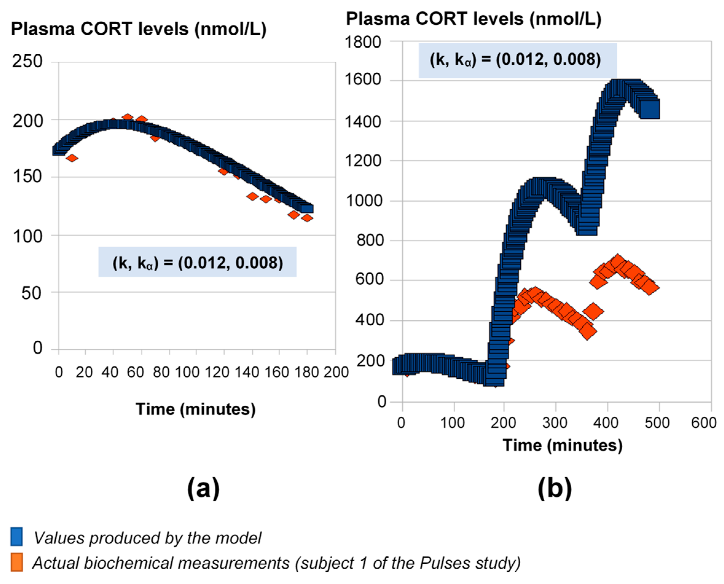
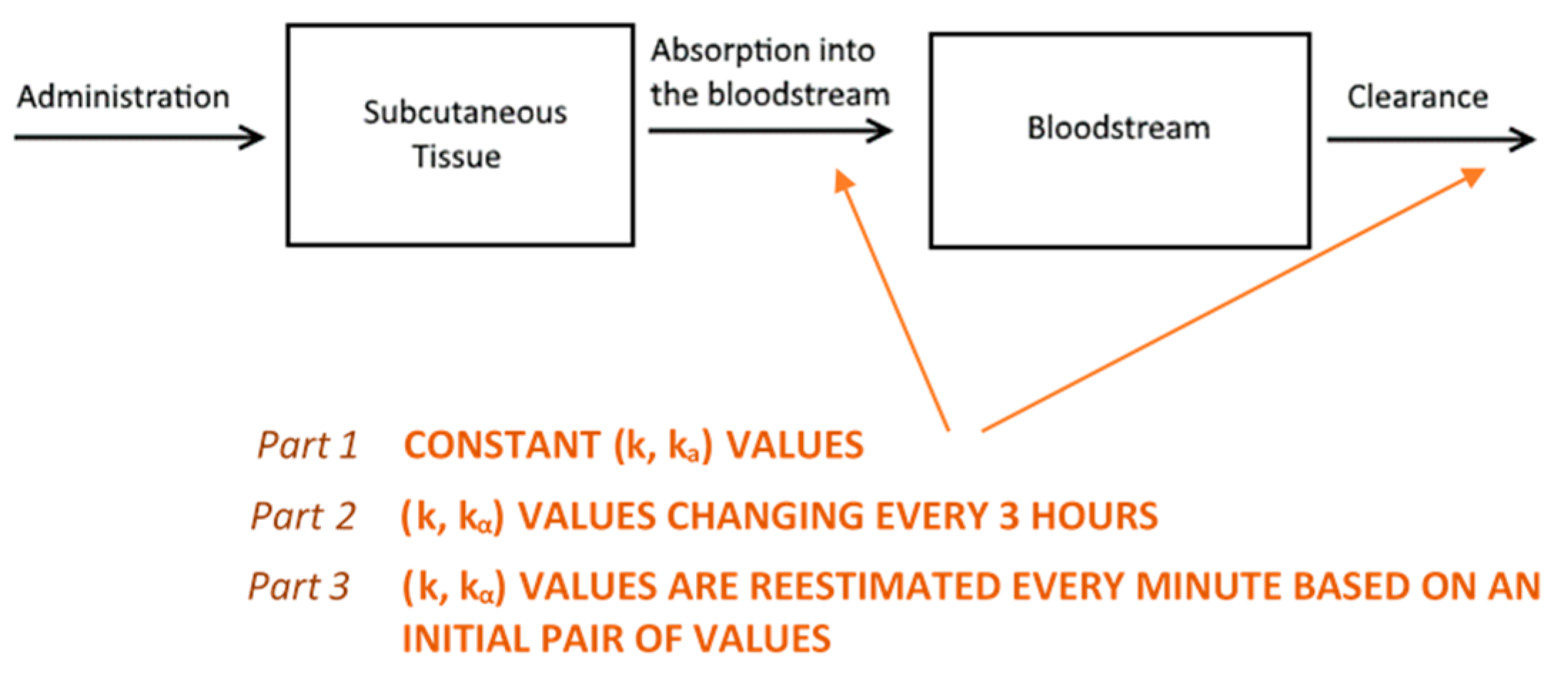
2.1. HC Delivery Assuming Constant Absorption and Clearance Rates

For this part of the study, we used the 24-h plasma cortisol profile of Subject 1 from the Pulses study (see Materials and Methods). First, we fitted the model parameters k and k_α using the initial 3 h of data (Figure 1a). If we continue the model simulations for the next 6 h of data using these rates, the model predictions diverge from the measured levels of plasma cortisol (Figure 1b).

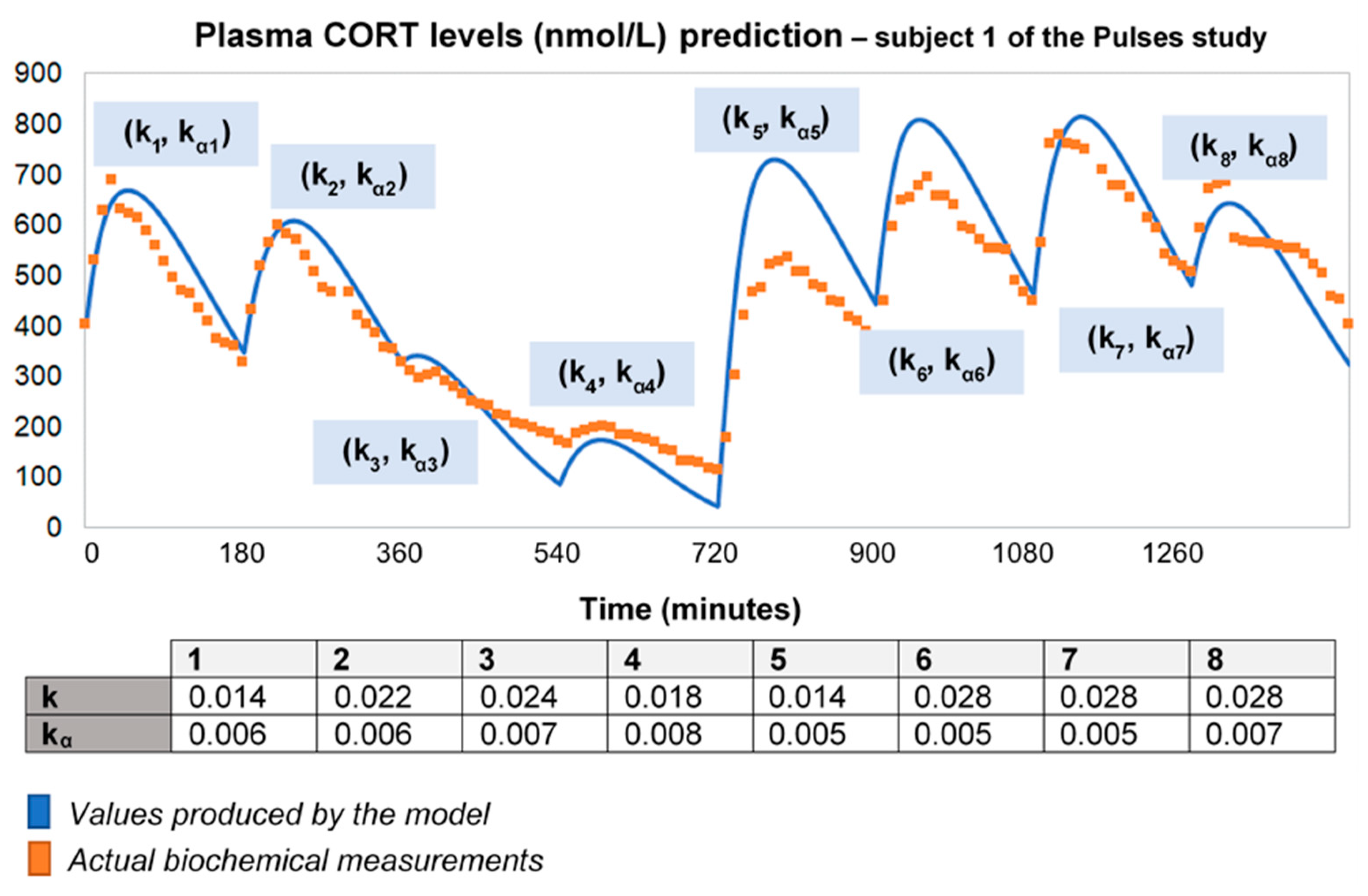
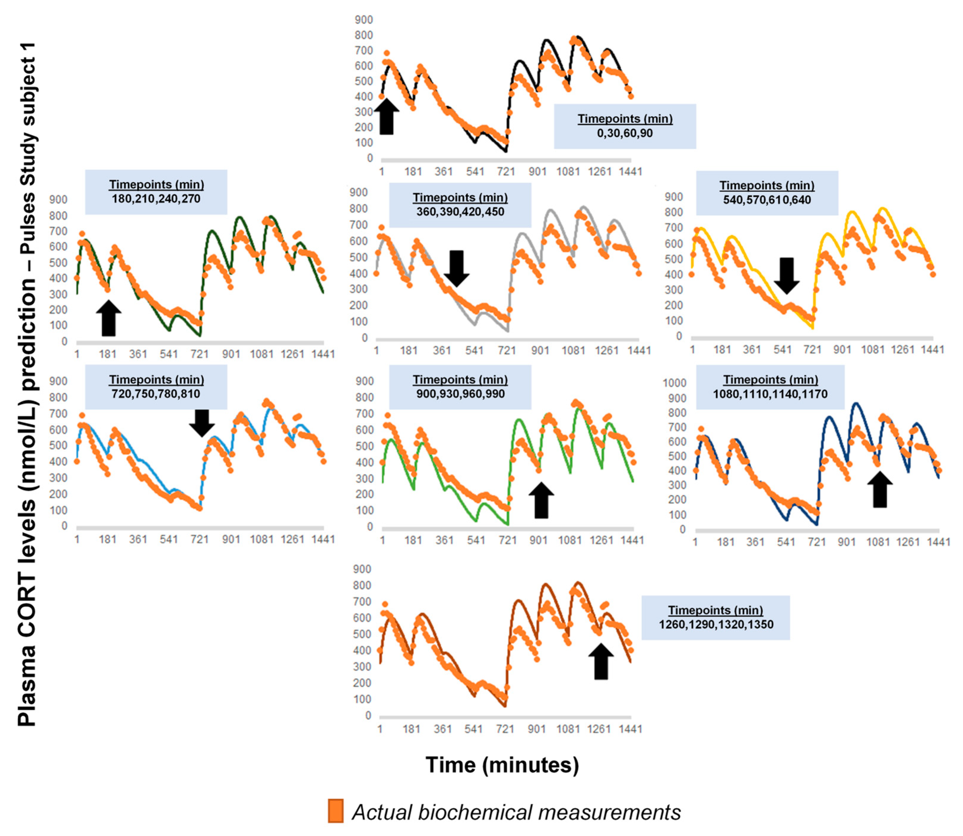
2.2. HC Delivery Assuming Piecewise Absorption and Clearance Rates That Change Every 3 h

To improve the output of the model for longer time intervals (using the 24-h plasma cortisol data of Subject 1 from the Pulses study), we needed to recalibrate the absorption and clearance rates every 3 h. This piecewise adjustment of model parameters improves the model fitting to data over 24 h (Figure 2). However, this is not an adequate process for a predictive model with minimal input.

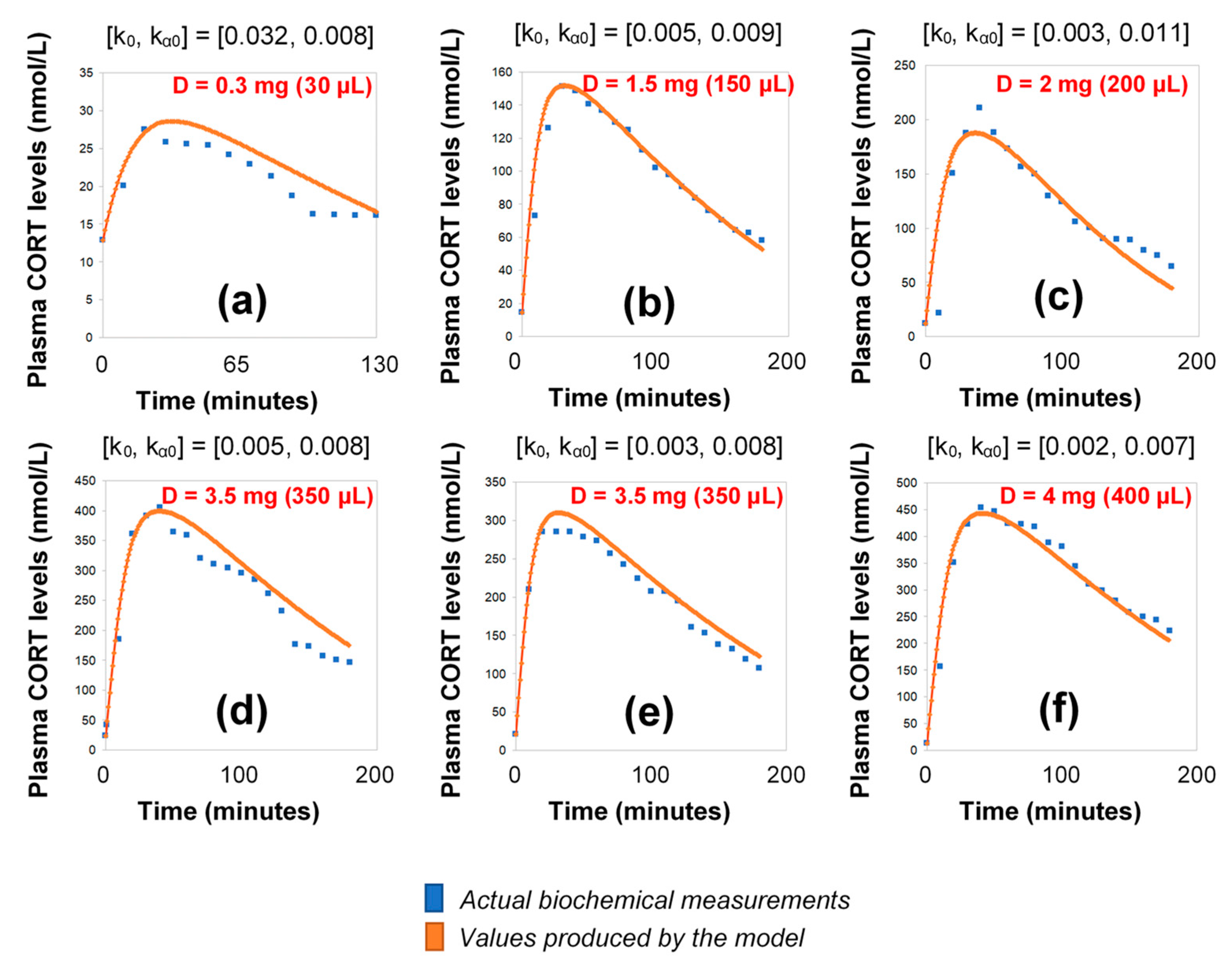
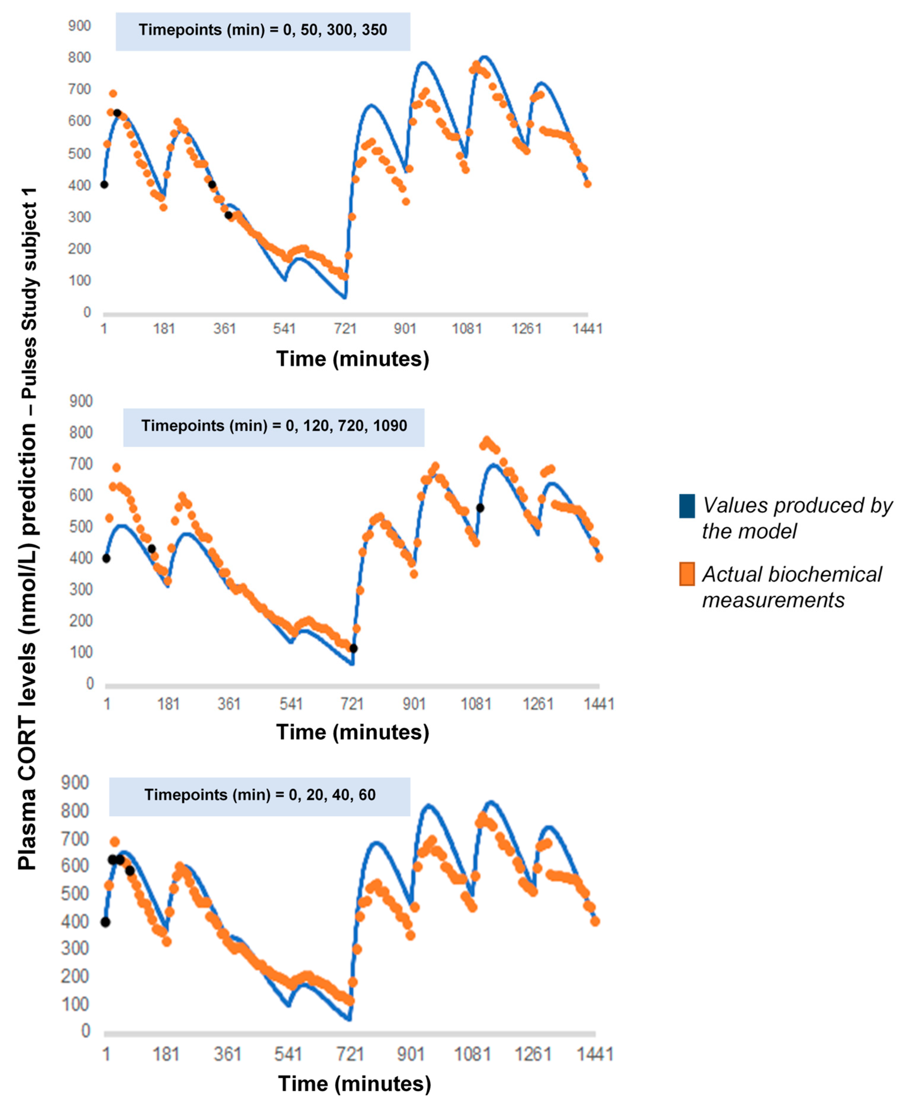
2.3. HC Delivery under Discretely Varying Absorption and Clearance Rates (Optimised Model)

Under the assumption of discretely varying absorption and clearance rates, we proceeded to recalibrate the model by computing just a single pair of initial (k₀, k_α0) for each individual (rather than every 3 h). To do this, we first used six 3-h healthy volunteer profiles with endogenous cortisol secretion suppressed by dexamethasone (Figure 3). Subsequently, we replicated the 24-h plasma cortisol profile of Subject 1 from the Pulses study by just estimating a single, initial pair of (k₀, k_α0). Specifically, we estimated k₀ = 0.016 and k_α0 = 0.0074 from only 4 plasma cortisol measurements (t₀, t₀ + 30 min, t₀ + 60 min and t₀ + 90 min). We chose t₀ as the first cortisol measurement (which was concurrent with the 15 h pulse from the pump) (Figure 4).

As a next step, we wanted to see how our model would behave if we chose a different combination of four cortisol measurements. We performed 7 runs, retaining the temporal relationship between the measurements (t₀, t₀ + 30 min, t₀ + 60 min and t₀ + 90 min) but shifting t₀ by 3 h every time to concur with a different pulse of the pump (t₀ = 180, 360, 540, 720, 900, 1080, 1260) (Appendix A). Finally, we performed 3 additional runs, retaining t₀ = 0 but changing the time distance between the four cortisol measurements: (1) reducing their in-between distance (t₀, t₀ + 20 min, t₀ + 40 min and t₀ + 60 min), (2) increasing their in-between distance (t₀, t₀ + 120 min, t₀ + 720 min and t₀ + 1090 min) and (3) having two distant pairs of cortisol values, each pair containing two proximal values (t₀, t₀ + 50 min, t₀ + 300 min and t₀ + 350 min) (Appendix B).

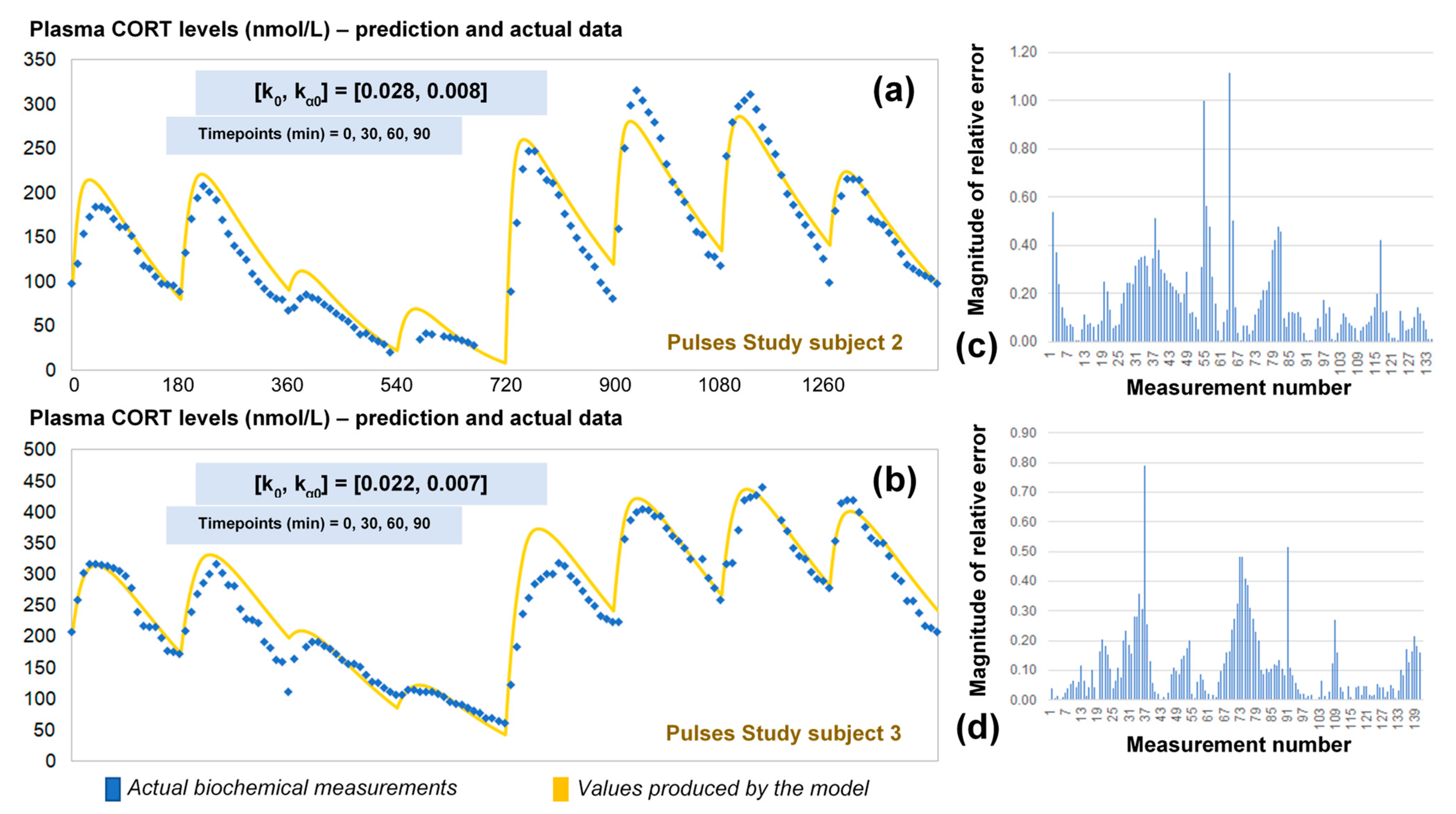
2.4. Validation of the Optimised Model for HC Delivery

The revised assumptions enabled the model to estimate plasma cortisol data through a simple and easy to use algorithm requiring only four data points as inputs. To validate our approach, we predicted the 24-h cortisol profile from the remaining two participants from the Pulses study (Figure 5). We did this by calculating the corresponding single pair of (k₀, k_α0) rates from only four plasma cortisol values measured at time points 0, 30 min, 60 min and 90 min. We also estimated the magnitude of the relative error for every time point of the model predictions versus the plasma cortisol data. Finally, the mean absolute error was estimated to be 14%.

2.5. Reaches and Limitations of the Model

A question that naturally arises is what is the best possible fit that our model can achieve. The process of finding this is straightforward given the following functions:

$$C_n\left(t,k_0,k_{a0}\right)=\frac{k_a\left(t\right)h}{k_a\left(t\right)-k\left(t\right)}\left({\displaystyle \sum }_{i=0}^n{\delta }_i\left(t\right)D_i\left(e^{-k\left(t\right)\left(t-t_i\right)}-e^{-k_a\left(t\right)\left(t-t_i\right)}\right)\right)+\sigma e^{-k\left(t\right)t}$$

(1)

M_i(t) is the i-th measurement taken every 10 intervals. We defined the error function for any n measurements as follows:

$$E_f\left(k_0,k_{a0}\right)={\displaystyle \sum }_{i=0}^n\frac{1}{n}{\left(C_i\left(t,k_0,k_{a0}\right)-M_i\left(t\right)\right)}^2$$

(2)

Therefore, we are interested in finding the ordered pair (k₀, k_α0) that minimizes this function, something that is achievable through basic multivariable calculus techniques.

3. Discussion

The use of smart, automated pumps for subcutaneous drug delivery is likely to expand over the next few decades as chronopharmacological research continues to provide new evidence on their therapeutic efficacy [17]. In various pathological conditions, smart pumps can improve drug administration by splitting it into multiple parts throughout the day (even during sleep), and by adjusting dose magnitude according to the time of the day and the patient’s internal time (e.g., pre-prandial vs. post-prandial states). These concepts are especially relevant to hormonal replacement therapies.

For the last 15 years, the scientific community has gathered multiple complementary pieces of evidence that support the notion that glucocorticoid pulsatility has biological significance [18], and thus chronopharmacological aspects in therapeutics involving glucocorticoids should be taken into serious consideration. In this context, pump-mediated glucocorticoid replacement strategies can replicate fast hormone secretion dynamics, thus offering certain advantages over other treatment approaches that disregard ultradian hormone pulsatility (e.g., oral substitution of HC twice or thrice daily or a pump-mediated continuous HC replacement).

Our group examined the scientific potential and challenges of pump-mediated dynamic hormone infusion through a series of clinical trials [13,16,19,20]. In these trials, either healthy volunteers with a pharmacologically disrupted capacity to produce glucocorticoids or patients with adrenocortical insufficiency underwent a pulsatile scheme of subcutaneous HC replacement. In the case of patients, this involved the daily infusion of 8 pulses of HC every 3 h, with varying doses depending on the time of the day. In these studies, patients were required to remain hospitalized for at least 24 h, while repeated blood samples were collected throughout the day. This continuous sampling allowed us to construct their daily plasma cortisol profile, and thus verify whether the pump-mediated treatment was replicating the desired hormonal dynamic pattern.

In this paper, we postulated a mathematical model that describes the pharmacokinetics of cortisol administration in adrenocortical insufficiency patients. We show how the model can be used to calibrate pump-mediated HC replacement, a necessary step for its adoption in clinical practice. Further, we presented an automated process to recalibrate the pump that optimizes plasma cortisol delivery for any individual given only four single time point measurements of plasma cortisol. In general, our model shows a reasonable accuracy (mean absolute percent error of 14%) in predicting 24 h long hormone profiles measured in patients (Figure 5). For smaller periods of time, the model accuracy can improve notoriously as seen from the simulations that lasted for 3 h (Figure 3). It is expected that small errors in our parameter estimations would invalidate the model predictions for long periods of time. Yet our model can give a good estimate for the pharmacokinetics of cortisol replacement in pump-mediated clinical trials that last up to 24 h.

Mathematical modelling can also shed light on our understanding of the physiological mechanisms underlying the dynamic absorption and clearance of subcutaneous HC. While both rates are likely to depend on individual differences (such as body mass index), our model suggests that the clearance rate varies throughout the day. During our model recalibration, we found the clearance can be affected by baseline levels of cortisol already in the bloodstream, while at the same time the rate of absorption seems to drop the more HC it is administered. The estimated rate of cortisol clearance is well within the predicted variability observed in previous studies [21]. It should also be noted that, while k can vary wildly among individuals, our model suggests that k_α variability arises less from individual differences and depends more on the given HC dose. On the other hand, the optimised model relies on the assumption that although the absorption and clearance rates change over time, these changes are discontinuous and therefore the constant rate model is a good approximation for small intervals of time. The algorithm used to estimate the initial (k, k_α) rates performs better when the input data points lie within a 30–40-min range, when they are associated to low cortisol levels and when at least one local maxima of the plasma cortisol profile is included. Similarly, the algorithm assumes that after 24 h the cortisol levels must return to a value close to the initial data point. This considerably minimises the error for the last 3 h of simulation. In general, the highest error is observed the further the distance from the initial data points and before the last 6 h of the 24-h period (i.e., at the interval from the 6-th to the 18-th hour from the beginning of the simulation).

Lastly, it is important to highlight that our model cannot predict plasma cortisol pulsatility if HC is administered in ways other than subcutaneously, or in individuals whose endogenous capacity to produce glucocorticoids is intact. This is because the well-defined subcutaneous infusion scheme would be confounded–both dynamically and quantitatively, with endogenous bursts of glucocorticoid secretion (affected by individual differences in lifestyle, gene expression, and experience of stressful events). The model may be solely used to predict and calibrate the pharmacokinetics of subcutaneous HC infusions in individuals with impaired endogenous steroidogenic capacity.

4. Materials and Methods

4.1. Participants and Interventions

We extracted plasma cortisol data from clinical trials performed at the University of Bristol (UK) over the past 7 years. These trials were performed in accordance with the highest bioethical and local institutional provisions, under the approval of the Medicines and Healthcare Products Regulatory Authority and according to the principles of Good Clinical Practice and the Declaration of Helsinki. These studies recruited: (1) patients with adrenocortical insufficiency (Addison’s disease and congenital adrenal hyperplasia) (Pulses study, IRAS ID: 98045, EudraCT No: 2012-001104-37, ISRCTN67193733), and (2) healthy volunteers whose endogenous cortisol secretion was suppressed via dexamethasone administration (IRAS ID: 106181, UKCRN-ID-15236). In the latter case, 1 mg of dexamethasone was received orally by healthy volunteers at midnight at their home, and 1 mg was administered at 9 a.m. the next day at the research unit, prior to the experiment. During the experiment, volunteers received two subcutaneous infusions of HC (via CANE pump, see below) at varying time intervals and doses (dose range 0.3–4 mg) over a 7-h period [16]. The first 3 h of plasma cortisol data following the first HC pulse were used in this study. In the case of patients with adrenocortical insufficiency, HC replacement therapy was administered over the course of 24 h in the same way (subcutaneously via the CANE pump, see below), but distributed in 8 pulses (i.e., doses) with a constant 3 h inter-pulse interval and three different dose amplitudes, a high dose (4 mg) at 03:00 a.m., 06:00 a.m. and 09:00 a.m., an intermediate dose (2.3 mg) at midday, 03:00 p.m. and 06:00 p.m. and a small dose (0.5 mg) at 09:00 p.m. and midnight [13].

4.2. Technical Specifications of Subcutaneous Hydrocortisone Delivery

A portable subcutaneous infusion pump (Crono P, CANE Applied Medical Technology Ltd., Cambridge, UK) containing 100 mg of HC in 1 mL (Efcortesol^®; Sovereign Medical Ltd., Stansted, Essex, UK) was made up to 10 mL with 0.9% saline and programmed to deliver a high-, medium- and low-sized pulse of HC. All pulses were delivered at a flow rate of 10 μL/s. The pump delivered HC subcutaneously via a cannula (Medtronic quick-set^®, Medtronic MiniMed, Northridge, CA, USA) inserted into the abdominal subcutaneous tissue.

4.3. Acquisition of Plasma Cortisol Data

During the experimental process, blood samples were collected via an intravenous cannula every 10 min for serum cortisol concentration estimation. Blood sampling was being performed by the human automated blood sampler (HABS) [19]. The latter is a multi-device system, controlled by a computer, dedicated to collect blood samples and substitute the amount of blood received with an equal amount of normal saline (containing NaCl 0.90% w/v). After each sampling session, samples were allowed to clot at room temperature prior to centrifugation and serum was frozen at −80 °C until assayed. Analysis was performed by an electrochemiluminescence immunoassay (Cobas^®, Roche Diagnostics Ltd., West Sussex, UK). Cross reactivity with 11-deoxycortisol was 4.1%.

4.4. Model Validation Strategy

The 24-h hormone profiles of 9 participants (6 healthy volunteers and 3 adrenal insufficiency patients) were used to validate the model as follows: randomly, one of the 24-h profiles was initially used to formulate the equation describing the circulating plasma cortisol concentration as a function of time. The 6 profiles from the healthy volunteer study were subsequently used to refine the pharmacokinetic model through model parameter estimations, optimisations and validation of the assumptions related to the absorption and clearance of cortisol. Finally, we tested the accuracy of the model to replicate the data from the two remaining 24-h profiles of the Pulses study (Figure 6).

4.5. Description of Parameters

Table 1. Biomodelling Parameters.

Parameter	Description	Means of Estimation	Units
C(t)	Plasma cortisol concentration as a function of time.	Predicted by the model	nmol/L
Sc(t)	Subcutaneous cortisol concentration as a function of time.	Predicted by the model	mg
Di	Hydrocortisone dosage	Known from the experiment	mg
kα(t)	Cortisol absorption rate in subcutaneous tissue. Real positive number.	Initial value fitted to data	1/min
k(t)	Plasma cortisol clearance rate. Real positive number.	Initial value fitted to data	1/min
t	Time	Self-explanatory	min
σ	Initial cortisol levels in the subjects’ bloodstream (C(0))	Known from the experiment	nmol/L
h	Unit conversion factor for concentration from mg to nmol/L in plasma. Real number, constant, h = 106/(362.42 × ℓ)	Self-explanatory	nmol/mg
ℓ	Plasma volume of a typical subject.	Estimated from the literature.	L

describes all parameters and state variables used in this work.

4.6. Mathematical Modelling

We based the formulation of the pharmacokinetic model on established biochemical principles [22]. Our approach involves a two-compartment model of sub-cutaneous and plasma GC dynamics. Starting from the simple assumption that GC absorption and clearance rates are constant (Part 1, see below), we proceed to show how considering them as variable improves the model predictive power (Parts 2 and 3, see below) (Figure 7). In all model simulations, we assumed a constant plasma volume of 3.025 L [23]. All simulations were produced using a computer program written in the C++ programming language.

4.6.1. Part 1

Initially, we assumed that both the rates of absorption and clearance are constant, and postulated the following system of ordinary differential equations to describe the underlying dynamics:

$$\frac{d{S}_c\left(t\right)}{dt}=-k_a{S}_c\left(t\right)$$

(3)

$$\frac{dC\left(t\right)}{dt}=-kC\left(t\right)+k_a{S}_c\left(t\right)$$

(4)

where S_c(t) and C(t) are the cortisol concentration in subcutaneous tissue and plasma, respectively. Both are measured in nmol/L. The rates of absorption and clearance are symbolized with k_α and k, respectively, and are considered constant.

Equation (3) is easily solvable, with

$$S_c\left(t\right)=D{e}^{-k_{a}t}$$

(5)

where D stands for the delivered HC dose measured in mg.

Substituting Equation (5) in (4) leads to the single differential equation:

$$\frac{dC\left(t\right)}{dt}+kC\left(t\right)=k_{a}D{e}^{-k_{a}t}$$

(6)

The solution to Equation (6) is derived in Appendix C and has the form:

$$C\left(t\right)=D\frac{k_a}{k_a-k}\left(e^{-kt}-e^{-k_{a}t}\right)+\sigma e^{-kt}$$

(7)

where σ denotes the initial cortisol measurement in plasma (σ = C(0)).

To predict the concentration of cortisol for an arbitrary number of sequential dosages, we generalize Equation (7) to:

$$C_n\left(t\right)=\frac{k_{a}h}{k_a-k}\left({\displaystyle \sum }_{i=1}^n{\delta }_i\left(t\right)D_i\left(e^{-k\left(t-t_i\right)}-e^{-k_a\left(t-t_i\right)}\right)\right)+\sigma e^{-kt}$$

(8)

where n is the number of dosages and h is a factor that converts the units of cortisol concentration from mg to nmol/L. The function δ_i(t) is a step function selecting for the i-th dose, with δ_i(t) = 1 if t ≥ t_i and δ_i(t) = 0 if t < t_i. The derivation of Equation (8) can be found in Appendix D. Using Equation (8), we simulated HC replacement throughout an entire day while keeping (k, k_α) constant.

4.6.2. Part 2

Using Equation (8), we produced a solution curve for every 3-h interval, which was fitted to the data by choosing different (k, k_α) pairs for each curve. Then, we concatenated the curves creating a fitted simulation with a duration of 24 h.

4.6.3. Part 3

In this part, we developed a more realistic model by introducing the following considerations: (i) Although the absorption and clearance rates change over time, these changes are discontinuous and hence the constant rate model can be a good approximation for small intervals of time. (ii) The clearance rate k varies proportionally to the concentration of cortisol in plasma. Furthermore, the assumption that better approximates the data is to use the maximum value of k(t) of all the values that have been calculated until now as shown below; which resets to its initial value k₀ every 24 h at 12:00 noon (in other words, k(t) can only increase, but not decrease, proportionally to C(t) until it resets every 24 h). (iii) The rate of absorption (k_α) depends on the moving boundary of a small sphere of liquid created within the subcutaneous tissue following HC delivery (Figure 8).

Based on consideration (ii), it follows that for K(t), a function such that $K\left(t\right)=k_0\frac{C\left(t-1\right)}{C\left(0\right)}$ for some initial concentration C(0) and for $x\in R$, the plasma cortisol clearance rate is given by $k\left(t\right)=max\{K\left(x\right):0<x\le t-1\}$ if t > 0 and k(t) = k₀ if t = 0. Then, if t = 1260 min (at 12:00 p.m.), $k\left(t\right)$ = $k_0$ (see also Appendix E). In relation to consideration (iii), we hypothesized that a small spherical pressure region is created within the subcutaneous tissue following the infusion of the HC solution [24,25,26,27].

The rate of absorption is dependent on the area of that receding sphere. Since the absorption rate is calculated as a percentage of cortisol at a given time, we postulated the following formula for time t and some constant $\widehat{v}$:

$$k_{\alpha }\left(t\right)=\frac{4\mathsf{\pi }r{\left(t\right)}^2}{V}\widehat{v}$$

(9)

The radius of the sphere in time t is denoted by r(t):

$$k_a\left(t\right)=\frac{4\mathsf{\pi }\widehat{v}{\left(r\left(t\right)\right)}^2}{\frac{4}{3}\mathsf{\pi }{\left(r\left(t\right)\right)}^3}=\frac{3\widehat{v}}{r\left(t\right)}$$

(10)

Since each HC dose is delivered by the infusion pump in the same place, r(t) is dependent on the dosage S_c(t) that remains in the subcutaneous compartment, which is a function of time. Taking into consideration that 1 mg of HC is contained in 100 μL of solution, r(t) can be expressed as:

$$r\left(t\right)={\left(\frac{75}{\mathsf{\pi }}\times S_c\left(t\right)\right)}^{\frac{1}{3}}$$

(11)

It follows that $k_a\left(t\right)={\left(\frac{S_c\left(0\right)}{S_c\left(t\right)}\right)}^{\frac{1}{3}}\times k_a\left(0\right)$ for some initial k_α(0) and initial dosage D(0) (see Appendix F).

Finally, based on our initial assumptions about k_α being dependent on the moving boundary of a small sphere, we estimated the volume in the subcutaneous tissue (see Appendix G) for any given time. To make calculations easier, we did that by estimating it once every minute.

A brute-force search algorithm checks the output of the model for different initial pairs of (k₀, k_α0), to minimize the error with the four actual cortisol values given as input, and then the whole 24-h curve is produced based on the chosen pair of (k₀, k_α0). Following this, the pair of (k, k_α) for every subsequent minute is calculated based on the algorithms provided in Appendix E and Appendix G.

5. Conclusions

In this paper, we introduce a pharmacokinetic model that predicts the 24-h plasma cortisol profile for patients with adrenocortical insufficiency under subcutaneous pulsatile HC replacement with good accuracy (mean absolute percent error of 14%), especially when only four plasma cortisol measurements are provided. This pharmacokinetic model can be used to support clinical trials or practice involving subcutaneous HC delivery in patients with reduced endogenous capacity to synthesize GCs.

References

1. Juszczak, G.R.; Stankiewicz, A.M. Glucocorticoids, genes and brain function. Prog. Neuropsychopharmacol. Biol. Psychiatry 2018, 82, 136–168. [Google Scholar] [CrossRef]
2. McEwen, B.S.; De Kloet, E.R.; Rostene, W. Adrenal steroid receptors and actions in the nervous system. Physiol. Rev. 1986, 66, 1121–1188. [Google Scholar] [CrossRef] [PubMed]
3. Roozendaal, B.; Hernandez, A.; Cabrera, S.M.; Hagewoud, R.; Malvaez, M.; Stefanko, D.P.; Haettig, J.; Wood, M.A. Membrane-associated glucocorticoid activity is necessary for modulation of long-term memory via chromatin modification. J. Neurosci. 2010, 30, 5037–5046. [Google Scholar] [CrossRef] [PubMed] [Green Version]
4. McMaster, A.; Jangani, M.; Sommer, P.; Han, N.; Brass, A.; Beesley, S.; Lu, W.; Berry, A.; Loudon, A.; Donn, R.; et al. Ultradian cortisol pulsatility encodes a distinct; biologically important signal. PLoS ONE 2011, 6, e15766. [Google Scholar] [CrossRef] [PubMed] [Green Version]
5. Chapman, K.; Holmes, M.; Seckl, J. 11β-hydroxysteroid dehydrogenases: Intracellular gate-keepers of tissue glucocorticoid action. Physiol. Rev. 2013, 93, 1139–1206. [Google Scholar] [CrossRef] [PubMed] [Green Version]
6. Conway-Campbell, B.L.; George, C.L.; Pooley, J.R.; Knight, D.M.; Norman, M.R.; Hager, G.L.; Lightman, S.L. The HSP90 molecular chaperone cycle regulates cyclical transcriptional dynamics of the glucocorticoid receptor and its coregulatory molecules CBP/p300 during ultradian ligand treatment. Mol. Endocrinol. 2011, 25, 944–954. [Google Scholar] [CrossRef] [Green Version]
7. Lightman, S.L.; Conway-Campbell, B.L. The crucial role of pulsatile activity of the HPA axis for continuous dynamic equilibration. Nat. Rev. Neurosci. 2010, 11, 710–718. [Google Scholar] [CrossRef]
8. Russell, G.M.; Kalafatakis, K.; Lightman, S.L. The importance of biological oscillators for hypothalamic-pituitary adrenal activity and tissue glucocorticoid response: Coordinating stress and neurobehavioural adaptation. J. Neuroendocrinol. 2015, 27, 378–388. [Google Scholar] [CrossRef] [Green Version]
9. Meijer, O.C.; Karssen, A.M.; de Kloet, E.R. Cell- and tIssue-specific effects of corticosteroids in relation to glucocorticoid resistance: Examples from the brain. J. Endocrinol. 2003, 178, 13–18. [Google Scholar] [CrossRef]
10. Walker, J.J.; Terry, J.R.; Lightman, S.L. Origin of ultradian pulsatility in the hypothalamic-pituitary-adrenal axis. Proc. Biol. Sci. 2010, 277, 1627–1633. [Google Scholar] [CrossRef] [Green Version]
11. Kalafatakis, K.; Russell, G.M.; Zarros, A.; Lightman, S.L. Temporal control of glucocorticoid neurodynamics and its relevance for brain homeostasis; neuropathology and glucocorticoid-based therapeutics. Neurosci. Biobehav. Rev. 2016, 61, 12–25. [Google Scholar] [CrossRef] [PubMed] [Green Version]
12. Crown, A.; Lightman, S. Management of patients with glucocorticoid deficiency. Nat. Clin. Pract. Endocrinol. Metab. 2005, 1, 62–63. [Google Scholar] [CrossRef] [PubMed]
13. Kalafatakis, K.; Russell, G.M.; Harmer, C.J.; Munafo, M.R.; Marchant, N.; Wilson, A.; Brooks, J.C.; Thai, N.J.; Ferguson, S.G.; Stevenson, K.; et al. Effects of the pattern of glucocorticoid replacement on neural processing; emotional reactivity and well-being in healthy male individuals: Study protocol for a randomised controlled trial. Trials 2016, 17, 44. [Google Scholar] [CrossRef] [PubMed] [Green Version]
14. Kalafatakis, K.; Russell, G.M.; Harmer, C.J.; Munafo, M.R.; Marchant, N.; Wilson, A.; Brooks, J.C.; Durant, C.; Thakrar, J.; Murphy, P.; et al. Ultradian rhythmicity of plasma cortisol is necessary for normal emotional and cognitive responses in man. Proc. Natl. Acad. Sci. USA 2018, 115, E4091–E4100. [Google Scholar] [CrossRef] [PubMed] [Green Version]
15. Russell, G.; Kalafatakis, K.; Thakrar, J.; Hudson, E.; Alim, L.; Marchant, N.; Thirard, R.; Brooks, J.; Thai, J.; Harmer, C.; et al. Differential effects of subcutaneous pulsatile versus oral hydrocortisone replacement therapy on fMRI resting state and task based emotional processing in patients with primary adrenal insufficiency. Endocrine Abstracts 2019, 65, OC2.1. [Google Scholar] [CrossRef]
16. Russell, G.M.; Durant, C.; Ataya, A.; Papastathi, C.; Bhake, R.; Woltersdorf, W.; Lightman, S. Subcutaneous pulsatile glucocorticoid replacement therapy. Clin. Endocrinol. 2014, 81, 289–293. [Google Scholar] [CrossRef] [Green Version]
17. Kim, D.W.; Zavala, E.; Kim, J.K. Wearable technology and systems modeling for personalized chronotherapy. Curr. Opin. Syst. Biol. 2020, 21, 9–15. [Google Scholar] [CrossRef]
18. Lightman, S.L.; Birnie, M.T.; Conway-Campbell, B.L. Dynamics of ACTH and Cortisol Secretion and Implications for Disease. Endocr. Rev. 2020, 41, 470–490. [Google Scholar] [CrossRef] [Green Version]
19. Henley, D.E.; Leendertz, J.A.; Russell, G.M.; Wood, S.A.; Taheri, S.; Woltersdorf, W.W.; Lightman, S.L. Development of an automated blood sampling system for use in humans. J. Med. Eng. Technol. 2009, 33, 199–208. [Google Scholar] [CrossRef]
20. Kalafatakis, K.; Russell, G.M.; Ferguson, S.G.; Grabski, M.; Harmer, C.J.; Munafo, M.R.; Marchant, N.; Wilson, A.; Brooks, J.C.; Thakrar, J.; et al. Glucocorticoid ultradian rhythmicity differentially regulates mood and resting state networks in the human brain: A randomised controlled clinical trial. Psychoneuroendocrinology 2021, 124, 105096. [Google Scholar] [CrossRef]
21. Dorin, R.I.; Qiao, Z.; Qualls, C.R.; Urban, F.K., 3rd. Estimation of maximal cortisol secretion rate in healthy humans. J. Clin. Endocrinol. Metab. 2012, 97, 1285–1293. [Google Scholar] [CrossRef] [PubMed]
22. Jambhekar, S.S.; Breen, P.J. Basic Pharmacokinetics, 2nd ed.; Pharmaceutical Press: London, UK, 2012. [Google Scholar]
23. Lemmens, H.J.M.; Bernstein, D.P.; Brodsky, J.B. Estimating blood volume in obese and morbidly obese patients. Obes. Surg. 2006, 16, 773–776. [Google Scholar] [CrossRef] [PubMed]
24. Thomsen, M.; Hernandez-Garcia, A.; Mathiesen, J.; Poulsen, M.; Sørensen, D.N.; Tarnow, L.; Feidenhans’l, R. Model study of the pressure build-up during subcutaneous injection. PLoS ONE 2014, 9, e104054. [Google Scholar] [CrossRef] [PubMed]
25. Leuenberger Jockel, J.P.; Roebrock, P.; Shergold, O.A. Insulin depot formation in subcutaneoue tissue. J. Diabetes. Sci. Technol. 2013, 7, 227–237. [Google Scholar] [CrossRef] [PubMed] [Green Version]
26. Shrestha, P.; Stoeber, B. Fluid absorption by skin tissue during intradermal injections through hollow microneedles. Sci. Rep. 2018, 8, 13749. [Google Scholar] [CrossRef] [PubMed]
27. Gradel, A.K.J.; Porsgaard, T.; Lykkesfeldt, J.; Seested, T.T.; Gram-Nielsen, S.; Kristensen, N.R.; Refsgaard, H.H.F. Factors Affecting the Absorption of Subcutaneously Administered Insulin: Effect on Variability. J. Diabetes Res. 2018, 1205121. [Google Scholar] [CrossRef]
28. Zhu, B.; Zhang, Q.; Pan, Y.; Mace, E.M.; York, B.; Antoulas, A.C.; Dacso, C.C.; O’Malley, B.W. A Cell-Autonomous Mammalian 12 hr Clock Coordinates Metabolic and Stress Rhythms. Cell. Metab. 2017, 25, 1305–1319.e9. [Google Scholar] [CrossRef] [Green Version]
Figure 1. Mathematical model predictions of plasma cortisol levels assuming constant absorption (kα) and secretion (k) rates. The model fits the data during the first three hours (a), but for the estimated (k, kα) values, it significantly deviates from the observed plasma cortisol values past the first three hours (b). Plasma cortisol measurements belong to Subject 1 from the Pulses study (see Materials and Methods). CORT: cortisol.
Pharmaceutics 13 00769 g001
Figure 2. To improve the fitting of the model for longer time intervals, we recalibrated the absorption and clearance rates every 3 h. Specifically, we used the model to produce a curve for every 3-h interval, which was then fitted to data with different (k, kα) pairs for each curve. Then, we concatenated the curves creating a piecewise fitted simulation with a duration of 24 h. Time points of delivery (magnitude of doses): 0 min (2.3 mg/230 μL), 180 min (2.3 mg/230 μL), 360 min (0.5 mg/50 μL), 540 min (0.5 mg/50 μL), 720 min (4 mg/400 μL), 900 min (4 mg/400 μL), 1080 min (4 mg/400 μL) and 1260 min (2.3 mg/230 μL). As before, plasma cortisol measurements from Subject 1 of the Pulses study were used. CORT: cortisol; k: clearance rate; kα: absorption rate.
Pharmaceutics 13 00769 g002
Figure 3. Simulation of plasma cortisol changes in different healthy subjects with pharmacologically suppressed cortisol biosynthesis with dexamethasone (see Materials and Methods) after the subcutaneous infusion of varying doses of hydrocortisone. The simulations were produced by the revised model (see Materials and Methods), which assumes discretely varying absorption and secretion rates of cortisol. (a) female subject, BMI: 20.4, pulse time: 10:00 a.m., pulse volume (D): 30 μL (0.3 mg); (b) male subject, BMI: 30, pulse time: 10:00 a.m., pulse volume (D): 150 μL (1.5 mg); (c) male subject, BMI: 22.5, pulse time: 10:30 a.m., pulse volume (D): 200 μL (2 mg); (d) male subject, BMI: 21.2, pulse time: 09:50 a.m., pulse volume (D): 350 μL (3.5 mg), (e) male subject, BMI: 23.3, pulse time: 10:10 a.m., pulse volume (D): 350 μL (3.5 mg); (f) female subject, BMI: 23.4, pulse time: 09:50 a.m., pulse volume (D): 400 μL (4 mg); BMI: body-mass index, CORT: cortisol, D: dose.
Pharmaceutics 13 00769 g003
Figure 4. Assuming discretely varying absorption and clearance rates (revised model), the brute-force search method provides the initial pair of (k0, kα0), based on four CORT measurements (e.g., at time points 0, 30, 60 and 90 min), and subsequently estimates the whole 24-h profile of plasma cortisol. The data from the Pulses study Subject 1 was used (see Materials and Methods). CORT: cortisol, k: clearance rate, kα: absorption rate. Time points of delivery (magnitude of doses): 0 min (2.3 mg/230 μL), 180 min (2.3 mg/230 μL), 360 min (0.5 mg/50 μL), 540 min (0.5 mg/50 μL), 720 min (4 mg/400 μL), 900 min (4 mg/400 μL), 1080 min (4 mg/400 μL), 1260 min (2.3 mg/230 μL).
Pharmaceutics 13 00769 g004
Figure 5. (a) Comparison of the revised model predictions (yellow line) with the ultradian rhythm of plasma cortisol observed in subject 2 (blue dots) from the Pulses study following subcutaneous pulsatile CORT infusion (see Materials and Methods). (b) Comparison of the revised model predictions (yellow line) with the ultradian rhythm of plasma cortisol observed in subjects 3 (blue dots) from the Pulses study following subcutaneous pulsatile CORT infusion (see Materials and Methods). The revised model assumes discretely varying absorption and clearance rates and the brut-force search method calculates the initial pair of (k0, kα0) rates by four cortisol measurements (for instance at timepoints 0, 30 60 and 90 min). We also estimated the relative error of the model predictions across all plasma cortisol data points for subject 2 (c) and 3 (d). The periodicity of the data allows us to assume that the value of cortisol 24 h later is the same as the first value given, and hence, the error is reduced as we approach the end of that 24-h period. CORT: cortisol, k: clearance rate, kα: absorption rate. Time points of delivery (magnitude of doses): 0 min (2.3 mg/230 μL), 180 min (2.3 mg/230 μL), 360 min (0.5 mg/50 μL), 540 min (0.5 mg/50 μL), 720 min (4 mg/400 μL), 900 min (4 mg/400 μL), 1080 min (4 mg/400 μL), 1260 min (2.3 mg/230 μL).
Pharmaceutics 13 00769 g005
Figure 6. Strategy for developing and optimising the pharmacokinetic model, describing the subcutaneous delivery of hydrocortisone (HC). (a) One of the 24-h cortisol profiles (blue diagram) was selected at random and used to formulate an equation describing plasma cortisol dynamics. We assumed constant rates of HC absorption and clearance and showed that such an approach cannot simulate reality. Three different scenarios were subsequently tested, of which only one was finally selected. (b) The selected optimised scenario assumes varying rates of HC absorption and clearance depending on the dose magnitude and circulating cortisol levels, respectively. The six 3-h healthy volunteer profiles (blue diagrams) under different subcutaneous doses of HC were used to validate these assumptions and confirm the reliability of the model. (c) Four plasma cortisol values from each of the remaining two patients with adrenocortical insufficiency were inputted into the model to predict their whole 24-h hormonal profile (red diagram). (d) The (theoretical) output of the model (red diagram) was compared to the actual 24-h plasma cortisol profile (blue diagram) of each of the two patients. HV: healthy volunteers.
Pharmaceutics 13 00769 g006
Figure 7. An illustration of the reasoning behind the two-compartment model. Hydrocortisone (HC) is administered into the subcutaneous tissue where it is absorbed with a rate of kα. Then, it is distributed via the bloodstream throughout the body, where it is cleared (by the liver and kidneys) with a rate k as predicted by the model. Initially, we assumed that both absorption and clearance rates were constant (part 1) and demonstrated why this is an unrealistic assumption. Following this, we proceeded to estimate a different ordered pair (k, kα) for every three-hour interval. Then, we concatenated the eight curves together to create a graph for a full day (part 2). Finally, we assumed that both rates change every minute (part 3), with the absorption rate depending on the magnitude of the dose administered and clearance rate depending on circulating cortisol levels.
Pharmaceutics 13 00769 g007
Figure 8. The reasoning behind the assumptions regarding the absorption rate of subcutaneous hydrocortisone (HC) administration. This rate depends on the subcutaneous dose magnitude, and the within-subject change in absorption rate with time. HC is a lipophilic molecule; its diffusion is hardly restricted by tissue membranes and thus can be assumed to be isotropic. Accordingly, we used a sphere as an approximation of the shape and movement of hormonal molecules infused into the subcutaneous tissue. Left: the higher the subcutaneous dose volume, the lower the absorption rate kα (kα is inversely proportional to the cubic root of the dose volume). When a small dose is administered by the pump cannula (e.g., 30 μL or 0.3 mg of HC) (a), the ratio of the area of the sphere to its volume is approximately 2.4-times greater than when a 13-times larger dose is administered (e.g., 400 μL or 4 mg of HC) (b). Therefore, the absorption rate drops to almost a similar degree (from about 0.01 to about 0.004). When administered in high doses, an increased fat deposition of the hormone could also contribute to dose-dependent changes in the absorption rate. Right: compared to the state where the absorption rate was considered constant and independent of the dosage, our assumption (of a dose-dependent kα) indicates that in lower doses, the absorption would be higher, while in higher doses would be lower (c). Part of the Figure has been created with BioRender.com.
Pharmaceutics 13 00769 g008